Abstract
In this paper, we have explored Noether symmetries for the Lagrangian corresponding to the Lemaitre-Tolman-Bondi (LTB) spacetime metric via a Rif tree approach. Instead of the frequently used method of directly integrating the Noether symmetry equations, a MAPLE algorithm is used to convert these equations to the reduced involutive form (Rif). The interesting feature of this algorithm is that it provides all possible metrics admitting different dimensional Noether symmetries. These metrics are given in the form of branches of a tree, known as a Rif tree. These metrics are used to solve the determining equations and the explicit form of symmetry vector fields are found, giving 4, 5, 6, 7, 8, 9, 11, and 17-dimensional Noether algebras. To add some physical implications, Einstein’s field equations are used to find the stress-energy tensor for all the explicitly known metrics, and the parameters appearing in the metrics are used to find bounds for different energy conditions.
PACS:
04.20.Jb
1. Introduction
The theory of general relativity is one of the most fundamental and accurate theories of gravity in modern physics. The beauty of this theory arises from its fabulous simplicity in describing gravitation in terms of geometry. Mathematically, this phenomenon can be interpreted by a statement that general relativity is based on the Einstein field equations (EFEs), which represent a system of ten non-linear partial differential equations, describing gravitation as a result of the interaction between spacetime geometry and the presence of mass and energy in its region. Due to their highly nonlinear nature, finding the exact solutions to EFEs is a difficult problem. However, a limited number of solutions to these equations are found in literature, using some symmetry restrictions [1]. These symmetries are defined in terms of a specific type of vector field, known as Killing vector fields (KVFs), which satisfy the condition [2]:
In the above equation, denotes the Lie derivative operator, V is a KVF, and is the metric tensor, where and vary from 0 to 3. Killing vector fields predict the conservation of energy of a physical system for it being invariant under time translation, while the conservation of linear and angular momenta respectively for a physical system is invariant under spatial translations and rotations in a spacetime.
Sometimes, conformal transformations are found to be helpful to find the conservation laws which are not obtained with the help of KVFs. For example, the conservation of energy does not appear as a time like KVF in the well-known Friedmann metric, but it can be recovered by applying some appropriate conformal transformation to this metric and then finding its Killing symmetries. Equivalently, one may directly find the conformal vector fields (CVFs) of the metric, defined by [2]:
where is a smooth map of spacetime coordinates. A CVF is called a homothetic vector field (HVF) if is constant. For different spacetime metrics, these three symmetries are thoroughly discussed in literature [3,4,5,6,7,8,9,10,11,12,13,14,15,16].
For every spacetime metric given by the corresponding Lagrangian is defined as where s denotes the arc length parameter and a dot over represents its derivative with respect to A vector field with its first prolongation where defines a Noether symmetry of the Lagrangian L provided that a gauge function exists satisfying the condition:
In the above equation, and are functions of s and the spacetime coordinates Like the above-defined spacetime symmetries, Noether symmetry is also used as a tool for finding exact solutions to EFEs and their classification. Noether symmetries are the symmetries of a Lagrangian corresponding to a spacetime metric and are of great importance on account of their link with conservation laws via Noether’s theorem [17]. For a Noether symmetry the associated conservation law is given by:
Apart from their major role in the classification of the exact solutions of EFEs, Noether symmetries are also helpful in solving complicated differential equations. In particular, these symmetries play an important role in reducing the order of ordinary differential equations, while in the case of partial differential equations they reduce the number of independent variables. Noether symmetries are also used in the linearization of nonlinear differential equations [18,19,20].
Some well-known relations between Noether and spacetime symmetries include: (i) Every KVF is a Noether symmetry but there may exist some Noether symmetries which are not KVFs, (ii) A vector field V is an HVF for a spacetime metric if and only if is a Noether symmetry for the associated Lagrangian [21], where signifies the homothety constant. A Noether symmetry that is not associated with an HVF and is different from a KVF is called a proper Noether symmetry. As for the conformal symmetries are concerned, they are not generally related to Noether symmetries except for the case of flat metric possessing 15 CVFs such that this set of 15 CVFs is properly contained in the set of 17 Noether symmetries for these spacetimes. Like spacetime symmetries, Noether symmetries are also explored for the Lagrangians associated with some spacetime metrics, the details can be seen in [22,23,24,25,26,27,28,29].
In this paper, we consider the most general LTB metric and explore the Noether symmetries of its associated Lagrangian. Instead of the frequently used method of directly integrating the determining equations, which is time-consuming and does not provide a complete classification, we follow a recently proposed approach that is based on a computer algorithm (Rif algorithm), developed in MAPLE using the “Exterior” package. The interesting feature of the Rif algorithm is that it analyzes the Noether symmetry equations and imposes certain conditions on the metric functions under which the system of Noether symmetry equations has a non-trivial solution. Such restrictions are given in terms of branches of a tree, known as a Rif tree. After that one needs to solve the symmetry equations under these restrictions. In this way, one gets all possible metrics along with their Noether symmetries of different dimensions, giving a complete classification of the spacetime under consideration.
2. Determining Equations and Rif Tree
The LTB metric can be written in the form [30,31,32]:
with three minimum KVFs, given by and In case when A and B depend only on the variable the above metric represents the Kantowski-Sachs spacetime [33] admitting an additional KVF Thus the present study also classifies the Kantowski-Sachs metric according to its Noether symmetries. The Lagrangian associated with the above metric is given by:
and the corresponding geodesic equations are:
where dot represents derivative with respect to affine parameter s. We use the expression with and in Equation (3) to get:
Substituting in the above equation, we obtain:
Using the expression for the Lagrangian given in Equation (6) in the above equation and simplifying it, we have:
Comparing the coefficients of , and the terms independent of we obtain the following Noether symmetry equations.
In order to find the explicit form of Noether symmetry generators, we need to solve the above equations. Because of their highly non-linear nature, these equations cannot be solved generally. In literature, such systems of equations are solved by imposing some conditions on A and with no proper criteria for imposing these conditions. This method is usually referred to as the direct integration technique. In this method, there is always a chance of losing some important spacetime metrics and hence it does not provide a complete classification of the spacetime under consideration. Here we follow a different approach to solve these equations. We analyze these equations by the Rif algorithm that gives a list of all possible metrics admitting different dimensional Noether algebras. The Rif algorithm was first introduced by Reid et al. [34] for converting a nonlinear system of differential equations to a simplified form (reduced involutive form ) by performing a finite number of differentiations and algebraic operations. The reduced involutive form of the system contains all the integrability conditions of the system and satisfies the constant-rank condition. To start the procedure, the system of differential equations is considered along with a matrix giving a complete ranking of the derivatives appearing in the system. After that, some differentiation and algebraic operations are carried out to simplify the system until it has all the integrability conditions included, with no more differential or algebraic redundancies. Though it is a quite lengthy procedure, the MAPLE command “rifsimp” and the “Exterior” package can be used to do all these calculations easily. There are many advantages of this algorithm, the most important being its role in reducing the complexity of the system and extracting the information about the number of its solutions, without solving it. The MAPLE command “caseplot” is used to see the output of the Rif algorithm graphically. This graph is always in the form of a tree, known as a Rif tree or classification tree. Performing these steps for the Noether symmetry Equations (11)–(25), we obtain the Rif tree given in Figure 1.
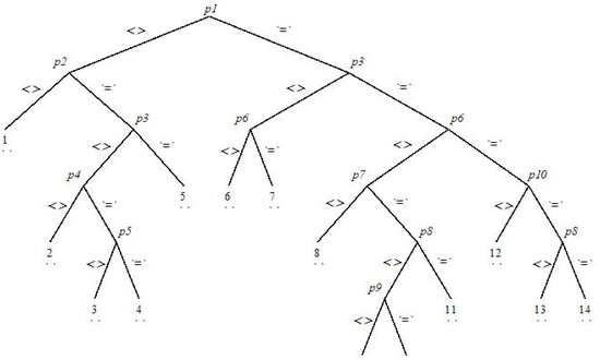
Figure 1.
Rif Tree.
The expressions for the nodes (pivots) of the above tree are given by:
It is to be mentioned here that in the Rif tree, the symbols = and tell about whether the corresponding pivot vanishes or it is non-zero. For example, and both are non-zero in branch 1, giving the conditions and on the metric functions. Similarly, different conditions are imposed on A and B by the remaining branches. We have used these restrictions on A and B, and solved Equations (11)–(25) for all 14 branches of the Rif tree. There are some branches in the tree which give rise to more than one metric with different dimensional Noether algebras. As a result, it is concluded that the possible dimensions of Noether algebras for the Lagrangian under consideration are 4, 5, 6, 7, 8, 9, 11, and 17. Depending upon the dimension of Noether algebra, we have summarized our results in the forthcoming sections. We have also compared our results with those obtained by the direct integration technique in Ref. [35] and it is observed that the Rif tree approach produces some new physically realistic metrics, not given by the direct integration technique.
3. 4-Dimensional Noether Algebra
The minimum dimension of Noether algebra for the spacetime under consideration is 4. This Noether algebra contains the minimum three KVFs of these spacetimes, given in the previous section, along with a trivial Noether symmetry This 4-dimensional Noether algebra is obtained for the metrics of branches 2, 3, and 8.
4. 5-Dimensional Noether Algebra
There are some branches whose constraints, while using to solve Equations (11)–(25), give rise to metrics possessing one additional symmetry along with four minimum Noether symmetries. In Table 1, we present all these metrics and their extra symmetry (denoted by ), which is purely a KVF. All the metrics in this section are Kantowski-Sachs metrics. The metrics 5a and 5c of Ref. [35] are specific forms of our metrics 5a and 5e respectively. The metric 5c reduces to the metric 5b of Ref. [35] when we take , and Moreover, the metrics 5f and 5g are the same as the metrics 5d and 5e of Ref. [35]. However, the metrics labeled by 5b and 5d are extra metrics that were not listed in Ref. [35].

Table 1.
Metrics Admitting five Noether Symmetries.
5. 6-Dimensional Noether Algebra
Like the case of five Noether symmetries, there are many branches of the Rif tree that produce metrics with two additional symmetries along with the four minimum Noether symmetries. These two extra symmetries are denoted by and and are listed in Table 2. For metric 6a, is a Noether symmetry corresponding to HVF, and is a KVF. For the metrics 6b-6h, is a proper Noether symmetry, and is a KVF, while the metric 6i, both and are proper Noether symmetries. The metrics 6a and 6b are respectively the same as the metrics 6c and 6d of Ref. [35]. The metrics 6e and 6g reduce to the metrics 6b and 6a of Ref. [35] for some specific value of B. Moreover, the metrics 6c, 6d, 6f, 6h, and 6i are extra metrics that were not found in Ref. [35] by using the direct integration technique.
Table 2.
Metrics Admitting Six Noether Symmetries.
6. 7-Dimensional Noether Algebra
During the process of integrating the determining equations, we found three different metrics possessing three additional symmetries along with the four minimum Noether symmetries. In Table 3, we present all these metrics and their additional three symmetries, denoted by , and For metrics 7a and 7b, is a proper Noether symmetry, is a Noether symmetry corresponding to an HVF, and gives a KVF. For metric 7c, is a Noether symmetry corresponding to an HVF, while and are KVFs. Moreover, all three additional symmetries for metric 7d are KVFs. Here, the metrics 7b and 7c are respectively the same as the metrics 7d and 7f of Ref. [35]. Moreover, the metric 7d recovers five metrics labeled by 7a, 7b, 7c, 7e, and 7g in Reference [35]. However, metric 7a is an extra metric obtained by the Rif tree approach.
Table 3.
Metrics Admitting Seven Noether Symmetries.
7. 8-Dimensional Noether Algebra
In this section, we present the metrics admitting four additional symmetries along with the four minimum ones. These four extra symmetries are denoted by ,..., in Table 4, along with the exact form of the metrics. For the metrics 8a–8d, corresponds to a HVF, is a KVF, while and are proper Noether symmetries. For the metric 8e, and are KVFs, while and represent proper Noether symmetries. The metrics 8c and 8d are the same as the metrics 8a and 8b of reference [35], while the metrics 8a, 8b, and 8e are extra metrics that were not listed in Ref. [35].
Table 4.
Metrics Admitting Eight Noether Symmetries.
8. 9-Dimensional Noether Algebra
Five branches of the Rif tree, labeled 6, 7, 11, 13, and 14 produce metrics possessing five additional symmetries along with the four minimum ones. In Table 5, we summarize the results of these five cases by listing the exact form of metrics and their additional symmetries. For metrics 9a and 9b, is a proper Noether symmetry and the remaining four are KVFs. For the remaining three metrics 9c–9e, , and are KVFs, while and denote proper Noether symmetries. The metrics 9a and 9b of Ref. [35] are respectively the special forms of the metrics 9b and 9a found here and the metrics 9c, 9d, and 9e are respectively the same as the metrics 9d, 9e, and 9c of Ref. [35].
Table 5.
Metrics Admitting Nine Noether Symmetries.
9. 11-Dimensional Noether Algebra
There arise two metrics, given by branches 4 and 7 possessing 11-dimensional Noether algebra. Out of these eleven, four are the minimum Noether symmetries and the extra seven symmetries are listed in Table 6. For metric 11a, represents a Noether symmetry corresponding to an HVF, and denotes a KVF. All the remaining symmetries are proper Noether symmetries. All the additional symmetries for metric 11b are KVFs. The metric 11b reduces to the metric possessing eleven Noether symmetries, given in Ref. [35], when we take , and , while the metric 11a is an extra metric which was not found by using direct integration technique.
Table 6.
Metrics Admitting Eleven Noether Symmetries.
10. 17-Dimensional Noether Algebra
Branch 5 of the Rif tree gives rise to a metric possessing 17-dimensional Noether algebra. Out of seventeen symmetries, four are the minimum ones, while thirteen additional symmetries, along with the exact form of metric coefficients are listed in Table 7. Here is a Noether symmetry corresponding to a HVF, given by are proper Noether symmetries, while are KVFs.
Table 7.
Metrics Admitting Seventeen Noether Symmetries.
11. Summary and Discussion
We have explored Noether symmetries of the Lagrangian associated with the LTB metric by using a new approach, based on a MAPLE algorithm, which provided a number of metrics possessing different Noether algebras with dimensions 4, 5, 6, 7, 8, 9, 11, and 17. After comparing our results with those obtained by the direct integration technique, it is concluded that this new approach produces some new LTB metrics admitting different dimensional Noether algebras which were not listed in the previous study using the direct integration technique.
For all the explicitly known metrics obtained during our classification, one can find the stress-energy tensor which determines the source of matter. Without specifying any specific matter, the non-zero components of the stress-energy tensor for the metric (5) are:
For an anisotropic fluid source, is of the form where , and are representing the energy density, four-velocity and spacelike unit vector respectively, and and are respectively the pressures parallel and perpendicular to . Also , and [36]. In particular, for the metric (5), the components of being an anisotropic fluid are given by Thus for the metrics representing anisotropic fluids, the off-diagonal component of stress-energy tensor vanishes and for such metrics one can easily calculate the quantities and as:
All the metrics obtained during our classification are anisotropic fluids with The physical soundness of such metrics can be checked by using the metric coefficients A and B in Equation (28) and then using the resulting values of and in the expressions for some well known energy conditions, for example null energy condition (NEC, ,), weak energy condition (WEC, ), strong energy condition (SEC, ) and dominant energy condition (DEC, ).
Some of our obtained metrics identically satisfy all the above-mentioned energy conditions. For example, consider the metric 6i given by:
For this metric, the components of energy-momentum tensor given in (27) become and . Hence Equation (28) gives and As the energy density is positive, the metric is physically realistic. Moreover, these values of and also satisfy all energy conditions. Similarly, the metrics labeled 8c, 8d, 8e, 9c, 9d, 9e, 11a, and 17a are also physically realistic metrics with positive energy density and satisfying all energy conditions. Out of these, metrics 11a and 17a represent vacuum solutions with vanishing stress-energy tensors.
Some of the obtained metrics are physically realistic with however the energy conditions for these metrics are conditionally satisfied. In Table 8, we present some of such metrics. One can see that the energy density is positive for metrics 5e, 7a, 7b, and 7d, giving physically realistic metrics. However, for the metrics 8a and 8b, we need to chose the constants and such that and The bound for energy conditions for all these metrics are given in Table 8.
Table 8.
Energy Conditions for Metrics.
Author Contributions
Investigation, M.F.; Methodology, A.M.; Software, N.M.; Supervision, T.H. All authors have read and agreed to the published version of the manuscript.
Funding
This research was funded by Prince Sultan University, Riyadh, Saudi Arabia through TAS LAB.
Institutional Review Board Statement
Not applicable.
Informed Consent Statement
Not applicable.
Data Availability Statement
Not applicable.
Acknowledgments
The authors N. Mlaiki and A. Mukheimer would like to thank Prince Sultan University for paying the publication fee for this work through TAS LAB. All the authors are thankful to the referees for their very useful suggestions.
Conflicts of Interest
The authors declare no conflict of interest.
References
- Stephani, H.; Kramer, D.; Maccallum, M.; Hoenselaers, C.; Herlt, E. Exact Solutions of Einstein’s Field Equations, 2nd ed.; Cambridge University Press: Cambridge, UK, 2003. [Google Scholar]
- Hall, G.S. Symmetries and Curvature Structure in General Relativity; World Scientific: London, UK, 2004. [Google Scholar]
- Feroze, T.; Qadir, A.; Ziad, M. The classification of plane symmetric spacetimes by isometries. J. Math. Phys. 2001, 42, 4947. [Google Scholar] [CrossRef]
- Deshmukh, S.; Belova, O. On killing vector fields on Riemannian manifolds. Sigma Math. 2021, 9, 259. [Google Scholar] [CrossRef]
- Nikonorov, Y.G. Spectral properties of Killing vector fields of constant length. J. Geom. Phys. 2019, 145, 103485. [Google Scholar] [CrossRef]
- Bokhari, A.H.; Qadir, A. Killing vectors of static spherically symmetric metrics. J. Math. Phys. 1990, 31, 1463. [Google Scholar] [CrossRef]
- Bokhari, A.H.; Qadir, A. Symmetries of static, spherically symmetric space–times. J. Math. Phys. 1987, 28, 1019. [Google Scholar] [CrossRef]
- Ahmad, D.; Ziad, M. Homothetic motions of spherically symmetric space–times. J. Math. Phys. 1997, 38, 2547. [Google Scholar] [CrossRef]
- Hall, G.S.; Steele, J.D. Homothety groups in space-time. Gen. Relativ. Gravit. 1990, 22, 457. [Google Scholar] [CrossRef]
- Bokhari, A.H.; Hussain, T.; Khan, J.; Nasib, U. Proper homothetic vector fields of Bianchi type I spacetimes via Rif tree approach. Results Phys. 2021, 25, 104299. [Google Scholar] [CrossRef]
- Usmani, A.A.; Rahaman, F.; Ray, S.; Nandi, K.K.; Kuhfittig, P.K.F.; Rakib, S.A.; Hasan, Z. Charged gravastars admitting conformal motion. Phys. Lett. B 2011, 701, 388–392. [Google Scholar] [CrossRef]
- Moopanar, S.; Maharaj, S.D. Conformal symmetries of spherical spacetimes. Int. J. Theor. Phys. 2010, 49, 1878–1885. [Google Scholar] [CrossRef][Green Version]
- Maartens, R.; Maharaj, S.D. Conformal killing vectors in Robertson-Walker spacetimes. Class. Quantum Gravity 1986, 3, 1005. [Google Scholar] [CrossRef]
- Saifullah, K.; Azdan, S.Y. Conformal motions in plane symmetric static space–times. Int. J. Mod. Phys. D 2009, 18, 71–81. [Google Scholar] [CrossRef]
- Coley, A.A.; Tupper, B.O.J. Spherically symmetric spacetimes admitting inheriting conformal Killing vector fields. Class. Quantum Gravity 1990, 7, 2195. [Google Scholar] [CrossRef]
- Maartens, R.; Mason, D.P.; Tsamparlis, M. Kinematic and dynamic properties of conformal Killing vectors in anisotropic fluids. J. Math. Phys. 1986, 27, 2987–2994. [Google Scholar] [CrossRef]
- Noether, E. Invariant variation problems. Invariant variation problems. Transp. Theory Stat. Phys. 1971, 1, 186–207. [Google Scholar] [CrossRef]
- Bluman, G.; Kumei, S. Symmetries and Differential Equations; Springer: New York, NY, USA, 1989. [Google Scholar]
- Wafo, S.C.; Mahomed, F.M. Linearization criteria for a system of second-order ordinary differential equations. Int. J. Non-Linear Mech. 2001, 36, 671–677. [Google Scholar]
- Ibragimov, N.H.; Maleshko, S.V. Linearization of third-order ordinary differential equations by point and contact transformations. J. Math. Anal. Appl. 2005, 308, 266–289. [Google Scholar] [CrossRef]
- Hickman, M.; Yazdan, S. Noether symmetries of Bianchi type II spacetimes. Gen. Relativ. Gravit. 2017, 49, 65. [Google Scholar] [CrossRef]
- Bokhari, A.H.; Kara, A.H. Noether versus Killing symmetry of conformally flat Friedmann metric. Gen. Relativ. Gravit. 2007, 39, 2053–2059. [Google Scholar] [CrossRef]
- Bokhari, A.H.; Kara, A.H.; Kashif, A.R.; Zaman, F.D. Noether symmetries versus Killing vectors and isometries of spacetimes. Int. J. Theor. Phys. 2006, 45, 1029–1039. [Google Scholar] [CrossRef]
- Camci, U.; Jamal, S.; Kara, A.H. Invariances and conservation laws based on some FRW universes. Int. J. Theor. Phys. 2014, 53, 1483–1494. [Google Scholar] [CrossRef]
- Ali, F.; Feroze, T.; Ali, S. Complete classification of spherically symmetric static space-times via Noether symmetries. Theor. Math. Phys. 2015, 184, 973–985. [Google Scholar] [CrossRef]
- Ali, S.; Hussain, I. A study of positive energy condition in Bianchi V spacetimes via Noether symmetries. Eur. Phys. J. C 2016, 76, 63. [Google Scholar] [CrossRef]
- Capozziello, S.; Marmo, G.; Rubano, C.; Scudellaro, P. Noether symmetries in Bianchi universes. Int. J. Mod. Phys. D 1997, 6, 491–503. [Google Scholar] [CrossRef]
- Capozziello, S.; Ritis, R.D.; Rubano, C.; Scudellaro, P. Noether symmetries in cosmology. Riv. Del Nuovo Cim. 1996, 19, 1–114. [Google Scholar] [CrossRef]
- Capozziello, S.; Piedipalumbo, E.; Rubano, C.; Scudellaro, P. Noether symmetry approach in phantom quintessence cosmology. Phys. Rev. D 2009, 80, 104030. [Google Scholar] [CrossRef]
- Lemaitre, G. The expanding universe. Gen. Relativ. Gravit. 1997, 29, 641. [Google Scholar] [CrossRef]
- Tolman, R.C. Effect of inhomogeneity on cosmological models. Proc. Natl. Acad. Sci. USA 1934, 20, 169–176. [Google Scholar] [CrossRef]
- Bondi, H. Spherically symmetrical models in general relativity. Mon. Not. R. Astron. Soc. 1947, 107, 410–425. [Google Scholar] [CrossRef]
- Kantowski, R.; Sachs, R.K. Some spatially homogeneous anisotropic relativistic cosmological models. J. Math. Phys. 1966, 7, 443–446. [Google Scholar] [CrossRef]
- Reid, G.J.; Wittkope, A.D.; Boulton, A. Reduction of systems of nonlinear partial differential equations to simplified involutive forms. Eur. J. Appl. Math. 1995, 7, 635–666. [Google Scholar] [CrossRef]
- Hussain, T.; Akhtar, S.S. Energy conditions and conservation laws in LTB metric via Noether symmetries. Eur. Phys. J. C 2018, 78, 677. [Google Scholar] [CrossRef]
- Coley, A.A.; Tupper, B.O.J. Spherically symmetric anisotropic fluid ICKV spacetimes. Class. Quantum Gravity 1994, 11, 2553. [Google Scholar] [CrossRef]

Publisher’s Note: MDPI stays neutral with regard to jurisdictional claims in published maps and institutional affiliations. |
© 2022 by the authors. Licensee MDPI, Basel, Switzerland. This article is an open access article distributed under the terms and conditions of the Creative Commons Attribution (CC BY) license (https://creativecommons.org/licenses/by/4.0/).