Analytical Study of Fractional Epidemic Model via Natural Transform Homotopy Analysis Method

Abstract

In this study, we present a new general solution to a rational epidemiological mathematical model via a recent intelligent method called the natural transform homotopy analysis method (NTHAM), which combines two methods: the natural transform method (NTM) and homotopy analysis method (HAM). To assess the precision and the reliability of the present method, we compared the obtained results with those of the Laplace homotopy perturbation method (LHPM) as well as the q-homotopy analysis Sumudu transform method (q-HASTM), which revealed that the NTHAM is more reliable. The Caputo fractional derivative is employed. It not only gives initial conditions with obvious natural interpretation but is also bounded, meaning that there is no derivative of a constant. The results show that the proposed technique is superior in terms of simplicity, quality, accuracy, and stability and demonstrate the effectiveness of the rational technique under consideration.

1. Introduction

Recently, there have been important efforts to enhance mathematical models in order to study the outbreak of transmissible disease [1,2,3]. Researchers have obtained important data for distinct contagious viruses via analyses of stochastic and deterministic models. Kermack and McKendrick [4] suggested a model beneficial for implementing and enhancing knotted epidemic models, which have been considered major models in the aspect of epidemiology to date. In recent years, there have been numerous epidemiological models, such as SIR [5,6,7,8], SIS [9], SEIR [10,11], SIRC [12], and other models [13,14,15,16,17], which generally depend on compartments. Many effective methods for obtaining numerical and analytical solutions for epidemic mathematical models with fractional-order derivatives have recently been used, for example, the Adomian decomposition method [18,19], homotopy perturbation technique [20], modified Laplace decomposition algorithm [21,22,23], homotopy analysis method (HAM) [24,25,26], q-HAM [27,28], q-homotopy analysis transform method [29], natural transform (NT) method [30], fractional residual power series method [31], q-homotopy analysis Sumudu transform method (q-HASTM) [32], q-homotopy analysis transform method (q-HATM) [33,34], Laplace Adomian decomposition method [35], natural transform decomposition method [36], fractional exponential function method [37], and Laplace homotopy perturbation method (LHPM) [38].

In this paper, we investigate a significant fractional mathematical model using a novel smart technique called the natural transform homotopy analysis method (NTHAM). It has general solutions for the NT method and HAM. The generalization of the proposed method is revealed by studying the current model using other techniques, such as the LHPM, and comparing the results. Now, we recall some fundamental notions. The Riemann–Lowville fractional integral operator of order $\alpha$ of a function $g(t)$ is defined by [39,40]:

$$I^{\alpha }g(t)=\frac{1}{\Gamma (\alpha )}{\displaystyle \underset{0}{\overset{t}{\int }}{(t-\tau )}^{\alpha -1}}g(\tau )d\tau ,(\alpha >0),\hspace{1em}{I}^{0}g(t)=g(t),$$

where $\Gamma$ is the gamma function, and $\alpha$ is an arbitrary but fixed base point. The integral is well-defined provided that $g$ is a locally integrable function, and $\alpha$ is a complex number in the half-plane $\mathrm{Re}(\alpha )>0$. The dependence on the base point $\alpha$ is often suppressed and represents freedom in the constant of integration. For the Riemann-Lowville fractional integral, we have: $I^{\alpha }{t}^{\gamma }=\frac{\Gamma (\lambda +1)}{\Gamma (\alpha +\lambda +1)}{t}^{\alpha +\lambda }.$ The fractional derivative of $g(t)$ in the Caputo sense is defined by [39,40]. $D^{\alpha }g(x)=J^{n-\alpha }{D}^{n}g(x)=\frac{1}{\Gamma (n-\alpha )}{\displaystyle \underset{a}{\overset{x}{\int }}{(x-t)}^{n-\alpha -1}}{g}^{(n)}(t) dt,(\alpha >0)$; $n-1<\alpha <n,n\in N,\alpha >0,a,\alpha ,t\in R,$ for example, the Caputo derivative $t^n$ is

$$D^{\alpha }{t}^n=\left\{\begin{array}{cc}0,& (n\le \alpha -1),\\ \frac{\Gamma (n+1)}{\Gamma (n-\alpha +1)}{t}^{n-\alpha },& (n>\alpha -1).\end{array}\right\}.$$

The fractional Caputo–Fabrizio derivative of order $\alpha$ is defined in [41] as follows:

Let $b>a, f\in H^1(a,b) ,$ and $\alpha \in (0,1)$. The fractional Caputo–Fabrizio derivative of order $\alpha$ for a function $f$ is defined by

$${}^{CF}{D}^{\alpha }f(t)=\frac{ M(\alpha )}{(1-\alpha )}{\displaystyle \underset{a}{\overset{t}{\int }}\exp (\frac{-\alpha }{1-\alpha }(t-s))}{f}^{\prime }(s) ds,$$

where $t\ge 0, M(\alpha ),$ which is a normalization function that depends on $\alpha$, and $M(0)=M(1)=1$.

If $f\notin H^1(a,b) ,$ and $0<\alpha <1$, this derivative can be presented for $f\in L^1(-\infty ,b)$ as ${}^{CF}{D}^{\alpha }f(t)=\frac{\alpha M(\alpha )}{(1-\alpha )}{\displaystyle \underset{a}{\overset{t}{\int }}(f(t)-f(s))\exp (\frac{-\alpha }{1-\alpha }(t-s))}ds$.

The Mittag-Leffler function $E_{\alpha }(z)$ with $\alpha >0$ is defined by the series representation, valid in the whole complex plane [42] $E_{\alpha }(z)={\displaystyle \sum _{k=0}^{\infty }\frac{z^k}{\Gamma (\alpha k+1)}}.$ A generalization of the Mittag-Leffler function $E_{\alpha }(z)={\displaystyle \sum _{k=0}^{\infty }\frac{z^k}{\Gamma (\alpha k+1)}}$, $\alpha \in C, R(\alpha )>0$, was introduced by Wiman [43] in the general form:

$$E_{\alpha ,\beta }(z)={\displaystyle \sum _{k=0}^{\infty }\frac{z^k}{\Gamma (\alpha k+\beta )}}, \alpha , \beta \in C, R(\alpha )>0,\hspace{1em}R(\alpha )>0.$$

Local fractional calculus is a modern field of mathematics that deals with derivatives and integrals of functions defined on fractal sets. Local fractional calculus (also called fractal calculus) was first presented by Kolwankar and Gangal [44]. In fractal space, the Gao-Yang-Kang local derivative of $g(x)$ of order $\alpha , 0<\alpha \le 1$ at $x=x_0$, is defined as [45,46,47]:

$$D_x^{\alpha }g(x)=g^{\alpha }(x)=\frac{d^{\alpha }g}{d{x}^{\alpha }}|{}_{x=x_0}={\lim }_{x\to x_0}\frac{{\mathsf{\Delta }}^{\alpha }(g(x)-g(x_0))}{{(x-x_0)}^{\alpha }},$$

where ${\Delta }^{\alpha }(g(x)-g(x_0))\cong \Gamma (\Theta +1) \Delta (g(x)-g(x_0)).$

LFD via the Caputo fractional derivative $D^{\alpha }$ of order $\alpha$ of a function $g(x)$ at point $x=a$ is usually defined by the following equation [48]:

$$(D^{\alpha }g)(a)={\lim }_{x\to a}{}_a{}^{RL}D{}_x^{\alpha }(g(x)-{\displaystyle \sum _{k=0}^{n-1}\frac{g^{(k)}(a)}{k!}}{(x-a)}^k),\hspace{1em}n-1<\alpha \le n,$$

where ${}_a{}^{RL}D{}_x^{\alpha }g(x)$ is the left side of the R-L fractional derivative of order $\alpha$, which is defined by [49]:

$${}_a{}^{RL}D{}_x^{\alpha }g(x)=\frac{1}{\Gamma (n-\alpha )} \frac{d^n}{d{x}^n}{\displaystyle {\int }_a^x\frac{g(\zeta )}{{(x-\zeta )}^{\alpha }}}d\zeta ,\hspace{1em}n-1<\alpha \le n.$$

A time scale is an arbitrary nonempty closed subset of real numbers. We denote a time scale [50] by the symbol T. The time-scale fractal derivative or Hausdorff derivative on the time fractal is defined as $\frac{\partial \mathrm{T}}{\partial t^{\sigma }}={\lim }_{x_B\to x_A}\frac{\mathrm{T}(t_B)-\mathrm{T}(t_A)}{{(t_B)}^{\sigma }-{(t_A)}^{\sigma }}$, where $\sigma$ is the fractal dimension of time. Another definition of the time-scale fractal derivative is introduced in [51,52,53,54,55]. There are significant roles for fractional differential equations (FDEs) in solving real-world problems [56,57,58]. This becomes obvious when using numerical approaches and comparing the relationships between various situations. Many studies have shown that using fractional-order derivatives produces better results in obtaining actual data for various models. The newly formulated Atangana–Baleanu derivative produces good results in many real-world problems. Fractional derivatives not only take into account the local characteristics of the dynamics but also consider the global evolution of the system; for that reason, when dealing with certain phenomena, they provide more accurate models of real-world behavior than standard derivatives. There are many applications of FDEs to different real-world problems, including chaotic ones, which have been reported in some fractional models.

2. Integral Transform Techniques

Integral transform techniques are frequently used for solving FDEs in various aspects of science. The major concepts of Laplace, Sumudu, and natural integral transforms are discussed using the following main concepts:

Definition 1.

The Laplace transform of a function $g(t), t\in (0,\infty )$ is defined by [39]:

$$L[f(t)](s)=F(s)={\displaystyle {\int }_0^{\infty }f(t) e^{-st}} dt, s\in C.$$

(1)

Definition 2.

The Laplace transform of the derivative of an integernof the function $f(t)$ [39] is:

$$L[D^{n}f(t)]=s^{n}F(s)-{\displaystyle \sum _{k=0}^{n-1}{s}^{n-k-1}}\hspace{1em}{f}^k(0)$$

(2)

Definition 3.

The Laplace transform of the Caputo fractional derivative is defined by [39]:

$$L[D^{\alpha }f(t)]=s^{\alpha }F(s)-{\displaystyle \sum _{k=0}^{n-1}{s}^{\alpha -k-1}}\hspace{1em}{f}^k(0),\hspace{1em}\hspace{1em}n-1<\alpha \le n$$

(3)

Definition 4.

In the early 1990s, Watugala [59] offered a new integral transform called the Sumudu transform, which has been applied to determine solutions of ODEs in control engineering problems. This Sumudu transform is defined over the set of functions:

$$A=\left\{f(t):\exists M,{\tau }_1,{\tau }_2>0,\left|f(t)\right|<M{e}^{\left|t\right|/{\tau }_j}, if t\in {(-1)}^j\times \left[0,\infty \right)\right\}$$

The Sumudu transform of$f(t)$is:

$$G(u)=S[f(t);u]={\displaystyle \underset{0}{\overset{\infty }{\int }}f(ut)e^{-t}}dt, u\in (-{\tau }_{1,},{\tau }_2).$$

(4)

Definition 5.

The Sumudu transform of the derivative of an integer n of the function $f(t)$ [60,61,62] is:

$$S[D_t^{n}f(t)]=u^{-n}S[f(t)]-{\displaystyle \sum _{k=0}^{n-1}{u}^{-\alpha +k}}{f}^{(k)}(0+)$$

(5)

Definition 6.

The Sumudu transform of the Caputo fractional derivative is [60,61,62]:

$$S[D_t^{\alpha }f(t)]=u^{-\alpha }S[f(t)]-{\displaystyle \sum _{k=0}^{n-1}{u}^{-\alpha +k}}{f}^{(k)}(0+).$$

(6)

Definition 7.

The natural transform method was initially defined by Khan and Khan [63], who studied its properties and applications. The main concepts of the natural transform (NT) and its characteristics are presented in [63,64,65,66,67,68,69,70,71].

Assume that $f(t)$ is a real function, $f(t)>0$ and $f(t)=0$ at $t<0$, section-wise continuous, of exponential order, and defined over the set of functions

$A=\left\{f(t):\exists M,{\tau }_1,{\tau }_2>0,\left|f(t)\right|<M{e}^{\left|t\right|/{\tau }_j}, if t\in {(-1)}^j\times \left[0,\infty \right)\right\}$ The natural transform of $f(t)$ is defined by:

$$N\left[f(t)\right]=R(s,u)={\displaystyle \underset{0}{\overset{\infty }{\int }}f(ut)e^{-st}dt}, u>0, s=0$$

(7)

where $N\left[f(t)\right]=R(s,u)$ is the natural transformation of the time function $f(t),$ and the variables $u$ and $s$ are the natural transform variables.

Definition 8.

Natural transform of $n$-derivative. If $f^n(t)$ is the $n$th derivative of function $f(t)$, then the natural transform of the n-derivative is given by:

$$N\left[f^n(t)\right]=R_n(s,u)=\frac{s^n}{u^n}R(s,u)-{\displaystyle \sum _{k=0}^{n-1}\frac{s^{n-(k+1)}}{u^{n-k}}{f}^{(k)}(0), n\ge 1.}$$

(8)

Definition 9.

If $N\left[f(t)\right]$ is the natural transform of a function, the natural transform of the fractional derivative of order $\alpha$ is defined as:

$$N\left[f^{\alpha }(t)\right]=\frac{s^{\alpha }}{u^{\alpha }}R(s,u)-{\displaystyle \sum _{k=0}^{\alpha -1}\frac{s^{\alpha -(k+1)}}{u^{\alpha -k}}{f}^{(k)}(0)}.$$

(9)

Definition 10.

If $R(s,u)$ is the natural transform and $F(s)$ is the Laplace transform of function $f(t)$ in A, then:

$$N\left[f(t)\right]=R(s,u)=\frac{1}{u}{\displaystyle \underset{0}{\overset{\infty }{\int }}f(t)e^{\frac{st}{u}}dt=}\frac{1}{u}F\left(\frac{s}{u}\right).$$

(10)

This is named the natural-Laplace duality (NLD).

Definition 11.

If $R(s,u)$ is the natural transform and $G(u)$ is the Sumudu transform of function $f(t)$ in A, then:

$$N\left[f(t)\right]=R(s,u)=\frac{1}{s}{\displaystyle \underset{0}{\overset{\infty }{\int }}f(\frac{ut}{s})e^{-t}dt=}\frac{1}{s}G\left(\frac{u}{s}\right)$$

(11)

This is called the natural-Sumudu duality (NSD).

By studying the relations between the Laplace, Sumudu, and natural transforms, we conclude that the NT is the general transform of both the ST and LT. At $u=1$ in Equations (8) and (9), we have the LT in Equations (2) and (3), and at $s=1$ in Equations (8) and (9), we have the ST in Equations (5) and (6). In sum, we can say that the LT, ST, and NT are symmetric to each other, as clarified in Equations (10) and (11).

3. Fractional Epidemic Model

Chen et al. [72] introduced a model and simulated data on transmission from the source of infection to the infection in people. In the present study, we assume that all parameters and variables involved in the model are non-negative in the individual community. The total population of individuals is considered $N(t)$, which is separated into five compartments: susceptible $E(t),$ exposed $H(t),$ symptomatic infected $\mathrm{Y}(t)$, asymptomatic infected $O(t)$, and recovered populations $F(t)$. The following assumptions were made in the model:

• The recruitment of individuals increases the size of the susceptible group at a constant rate $\Pi$.
• The childbirth rate and natural mortality rate of individuals are indicated by parameters $\mu$ and $\delta$, respectively.
• A susceptible individual is infected over numerous contacts with infected individuals $\mathrm{Y}(t)$ via the given term $\beta \frac{E(t)Y(t)}{N}$, where the contact rate $\beta$ is the disease transmission coefficient.
• Transmission from an asymptotic infected individual $O(t)$ to a susceptible individual $E(t)$ can take place in the form $\beta \frac{E(t)Y(t)}{N}$, where $\psi \notin \left[0,1\right]$ is a transmissibility multiple of $O(t)$ to $\mathrm{Y}(t)$; if $\psi =0$, no transmissibility multiple will exist and thus vanish, and if $\psi =1$, then a transmissibility multiple will exist.
• The parameter $\varphi$ is the proportion of asymptotic infections. The parameters $\theta$ and $\vartheta$ respectively indicate the transmission rate after the incubation period and joining classes $\mathrm{Y}(t)$ and $O(t)$.
• Individuals in the symptomatic group $\mathrm{Y}(t)$ and asymptomatic group $O(t)$ are removed at recovery rates of $\gamma$ and $\tau$ and are added to the recovered $F(t)$ compartment.
• A susceptible individual will be infected after interaction with the reservoir or the seafood place or market class $G(t)$ through the term given by $\eta \frac{E(t)Y(t)}{N}$, where $\eta$ is the disease transmission coefficient from $E(t)$ to $G(t)$. $\mathrm{Y}(t)$ and $O(t)$ individuals transmit the virus to the reservoir or the seafood place or market class $G(t)$ at constant rates of $\sigma$ and $\epsilon$, respectively.
• The removal rate of the virus from the reservoir or the seafood place or market class $G(t)$ is indicated by $k$. Using the above assumptions, the mathematical representation of the model comprising the fractional-order dynamical system is [32,33]:

$$\begin{array}{l}{D}_t^{\alpha }E(t) =\Pi -\beta \frac{EY}{N}- \beta \psi \frac{EO}{N}-\eta \frac{EG}{N}-\delta E\\ D_t^{\alpha }H(t)=\beta \frac{EY}{N}+\beta \psi \frac{EO}{N}+\eta \frac{EG}{N}-(1-\varphi ) \theta H-\varphi \vartheta H-\delta H\\ D_t^{\alpha }Y(t)=(1-\varphi ) \theta H-\gamma Y-\delta Y\\ D_t^{\alpha }O(t)=\varphi \vartheta H-a O-\delta O\\ D_t^{\alpha } F(t)=\gamma Y+a O-\delta F\\ D_t^{\alpha }G(t)=\sigma Y+\epsilon O-k G,\hspace{1em}\hspace{1em}\hspace{1em}\hspace{1em}\hspace{1em}\hspace{1em}\hspace{1em}\hspace{1em}0<\alpha \le 1\end{array}$$

(12)

with the initial conditions

$$E(0) =E_0 , H(0)=H_0 , Y(0)=Y_0 , O(0)=O_0,F(0)=0,G(0)=0.$$

(13)

The population compartments can be normalized by $N$ by adopting the current state variables:

$$M=\frac{E}{N},Q=\frac{H}{N},R=\frac{Y}{N},S=\frac{O}{N},\varpi =\frac{F}{N},{\rm Z}=\frac{G}{N},\xi =\frac{\Pi }{N}.$$

(14)

The population is normalized and transformed into the non-dimensional form as follows:

$$\begin{array}{l}{D}_t^{\alpha }M =\xi -\beta M R- \beta \psi M S-\eta M {\rm Z}-\delta M\\ D_t^{\alpha }Q=\beta M R+\beta \psi M S+\eta M {\rm Z}-(1-\varphi ) \theta Q-\varphi \vartheta Q-\delta Q\\ D_t^{\alpha }R=(1-\varphi ) \theta Q-\gamma R-\delta R\\ D_t^{\alpha }S=\varphi \vartheta Q-a S-\delta S\\ D_t^{\alpha } \varpi =\gamma R+a S-\delta \varpi \\ D_t^{\alpha }{\rm Z}=\sigma R+\epsilon S-k {\rm Z}\hspace{1em}\hspace{1em}\hspace{1em}\hspace{1em}\hspace{1em}\hspace{1em}\hspace{1em}\hspace{1em}0<\alpha \le 1\end{array}$$

(15)

with the following initial conditions:

$$\begin{array}{l}M(0)=M_o\ge 0 ,Q(0)=Q_0\ge 0, R(0)=R_0\ge 0,\\ S(0)= S_0\ge 0, \varpi (0)= {\varpi }_0\ge 0, {\rm Z}(0)= {{\rm Z}}_0\ge 0.\end{array}$$

(16)

The fitted and estimated values of parameters and the initial conditions for the model with the fractional-order derivative are taken from Ref. [32].

4. Methodology of the Proposed Method

Consider the following nonlinear differential equation:

$$\ell \mathsf{\Psi }+\Re \mathsf{\Psi }+\Im \mathsf{\Psi }=\delta (x),$$

(17)

where $\ell$ is a linear differential operator, $\Re$ is the residual of the linear operator, $\Im$ is the nonlinear term, and $\delta (x)$ is the source term. Applying NT to both sides of Equation (17), we obtain:

$$N[\ell \mathsf{\Psi }+\Re \mathsf{\Psi }+\Im \mathsf{\Psi }]=N[\delta (x)].$$

(18)

After simplifying, we have

$$N[\mathsf{\Psi }]-\frac{u^m}{s^m}{\displaystyle \sum _{\eta =0}^{m-1}\frac{s^{m-(\eta +1)}}{u^{m-\eta }}}{\mathsf{\Psi }}_t{}^{(\eta )}(x,0)+\frac{u^m}{s^m}[N[\Re \mathsf{\Psi }]+N[\Im \mathsf{\Psi }]-N[\delta (x)]]=0,$$

(19)

We define the nonlinear operator

$$\begin{array}{l}\Im [\mathsf{\Phi }(x,t;q)]=N[\mathsf{\Phi }(x,t;q)]-\frac{u^m}{s^m}{\displaystyle \sum _{\eta =0}^{m-1}\frac{s^{m-(\eta +1)}}{u^{m-\eta }}}{\mathsf{\Phi }}_t{}^{(\eta )}(x,0;q)\\ +\frac{u^m}{s^m}[N[\Re \mathsf{\Phi }(x,t;q)]+N[\Im \mathsf{\Phi }(x,t;q)]-N[\delta (x)]]\\ +N[\Im \mathsf{\Phi }(x,t;q)]-N[\delta (x)]],\end{array}$$

(20)

where $q\in [0,1],$ and $\mathsf{\Phi }(x,t;q)$ is a real function of $x,t$ and $q$.

We set a homotopy as follows:

$$(1-q) N [\mathsf{\Phi }(x,t;q)-{\mathsf{\Psi }}_0(x,t)] =q ħ H(x,t) \Im [\mathsf{\Phi }(x,t;q)],$$

(21)

where $q\in [0,1]$ represents the embedding parameter, and $ħ\ne 0$ is an auxiliary parameter. The role of the auxiliary parameter $ħ$ is based on homotopy, a basic concept of topology. The nonzero auxiliary parameter is introduced to construct the so-called zero-order deformation equation, which gives a more general homotopy than the traditional one. $N$ denotes the natural transform, ${\mathsf{\Psi }}_0(x,t)$ is the initial guess of $\mathsf{\Psi }(x,t)$, $\mathsf{\Phi } (x,t;q)$ denotes an unknown function of $x, t$, and $H(x,t)$ is a nonzero auxiliary function. When the embedding parameters are $q=0$ and $q=1$, it respectively holds that

$$\mathsf{\Phi }(x,t;0)={\mathsf{\Psi }}_0(x,t),\mathsf{\Phi }(x,t;1)={\mathsf{\Psi }}_1(x,t).$$

(22)

Thus, as $q$ increases from $0$ to $1$, the solution $\mathsf{\Phi } (x,t;q)$ varies from the initial guess ${\mathsf{\Psi }}_0(x,t)$ to the solution $\mathsf{\Phi }(x,t;q)$. If we expand $\mathsf{\Phi }(x,t;q)$ in the Taylor series with respect to $q$, we have

$$\mathsf{\Phi } (x,t,q)={\mathsf{\Psi }}_0(x,t)+{\displaystyle \sum _{n=1}^{\infty }{\mathsf{\Psi }}_n(x,t) q^{n } ,}$$

(23)

where

$${\mathsf{\Psi }}_n(x,t)={\frac{1}{n!}\frac{{\partial }^n\mathsf{\Phi }(x,t,q)}{\partial q^n}|}_{q=0}$$

(24)

If the auxiliary linear operator, initial guess, auxiliary parameter $ħ,$ and auxiliary function are properly chosen, Series (24) converges at

$$\mathsf{\Psi }(x,t)={\mathsf{\Psi }}_0(x,t)+{\displaystyle \sum _{n=1}^{\infty }{\mathsf{\Psi }}_n(x,t)}.$$

(25)

The vectors are defined as follows:

$$\overrightarrow{{\mathsf{\Psi }}_n}=\{{\mathsf{\Psi }}_0(x,t),{\mathsf{\Psi }}_1(x,t),{\mathsf{\Psi }}_2(x,t),\dots ,{\mathsf{\Psi }}_n(x,t)\}.$$

(26)

Differentiating Equation (20) $n$ times with respect to $q,$ dividing by $n!,$ and setting $q=0$, we obtain the following $n$th-order deformation equation:

$$N[{\mathsf{\Psi }}_n(x,t)-x_n {\mathsf{\Psi }}_{n-1}(x,t)]=ħ {\mathsf{\Omega }}_n({\mathsf{\Psi }}_{n-1}^{\to }),$$

(27)

where

$${\mathsf{\Omega }}_n({\mathsf{\Psi }}_{n-1}^{\to })=\frac{1}{n!}{\frac{{\partial }^{n-1}\Im [\mathsf{\Phi }(x,t,q)]}{\partial q^{n-1}}|}_{q=0}, x_n=\{\begin{array}{l}0, n\le 1\\ 1, n>1\end{array}$$

(28)

Applying the inverse natural transform, we have

$${\mathsf{\Psi }}_n(x,t)=x_n {\mathsf{\Psi }}_{n-1}(x,t)+ħ N^{-1}[{\mathsf{\Omega }}_n({\mathsf{\Psi }}_{n-1}^{\to })],n=1,2,3,\dots$$

(29)

5. Solution of the Fractional Epidemiological Model (FEM) via NTHAM

Applying the NT of Equation (15), we obtain:

$$\begin{array}{l}N[M]-\frac{u^{\alpha }}{s^{\alpha }}{\displaystyle \sum _{\upsilon =0}^{\alpha -1}\frac{s^{\alpha -(\upsilon +1)}}{u^{\alpha -\upsilon }}{M}_{\tau }^{(\upsilon )}(0)}-\frac{u^{\alpha }}{s^{\alpha }}N[\xi -\beta M R- \beta \psi M S-\eta M {\rm Z}-\delta M]=0,\\ N[Q]-\frac{u^{\alpha }}{s^{\alpha }}{\displaystyle \sum _{\upsilon =0}^{\alpha -1}\frac{s^{\alpha -(\upsilon +1)}}{u^{\alpha -\upsilon }}{Q}_{\tau }^{(\upsilon )}(0)}-\frac{u^{\alpha }}{s^{\alpha }}N[\beta M R+\beta \psi M S+\eta M {\rm Z},\\ -(1-\varphi ) \theta Q-\varphi \vartheta Q-\delta Q]=0\\ N[R]-\frac{u^{\alpha }}{s^{\alpha }}{\displaystyle \sum _{\upsilon =0}^{\alpha -1}\frac{s^{\alpha -(\upsilon +1)}}{u^{\alpha -\upsilon }}}{R}_{\tau }^{(\upsilon )}(0)-\frac{u^{\alpha }}{s^{\alpha }}N[(1-\varphi ) \theta Q-\gamma R-\delta R]=0,\end{array}$$

(30)

$$\begin{array}{l}N[S]-\frac{u^{\alpha }}{s^{\alpha }}{\displaystyle \sum _{\upsilon =0}^{\alpha -1}\frac{s^{\alpha -(\upsilon +1)}}{u^{\alpha -\upsilon }}}{S}_{\tau }^{(\upsilon )}(0)-\frac{u^{\alpha }}{s^{\alpha }}N[\varphi \vartheta Q-a S-\delta S]=0\\ N[\varpi ]-\frac{u^{\alpha }}{s^{\alpha }}{\displaystyle \sum _{\upsilon =0}^{\alpha -1}\frac{s^{\alpha -(\upsilon +1)}}{u^{\alpha -\upsilon }}{\varpi }_{\tau }^{(\upsilon )}}(0)-\frac{u^{\alpha }}{s^{\alpha }}N[\gamma R+a S-\delta \varpi ]=0\\ N[{\rm Z}]-\frac{u^{\alpha }}{s^{\alpha }}{\displaystyle \sum _{\upsilon =0}^{\alpha -1}\frac{s^{\alpha -(\upsilon +1)}}{u^{\alpha -\upsilon }}{{\rm Z}}_{\tau }^{(\upsilon )}}(0)-\frac{u^{\alpha }}{s^{\alpha }}N[\sigma R+\epsilon S-k {\rm Z} ]=0.\end{array}$$

(31)

Now, we define the nonlinear operator as follows:

$$\begin{array}{l}\Im [{\Theta }_1(t;q)]=N[{\Theta }_1(t;q) ]-\frac{u^{\alpha }}{s^{\alpha }}{\displaystyle \sum _{\upsilon =0}^{\alpha -1}\frac{s^{\alpha -(\upsilon +1)}}{u^{\alpha -\upsilon }}{\Theta }_{1,t}^{(\upsilon )}(0)}\\ -\frac{u^{\alpha }}{s^{\alpha }}N[\xi -\beta {\Theta }_1(t;q) {\Theta }_3(t;q)- \beta \psi {\Theta }_1(t;q) {\Theta }_4(t;q)\\ -\eta {\Theta }_1(t;q) {\Theta }_6(t;q)-\delta {\Theta }_1(t;q)]\\ \Im [{\Theta }_2(t;q)]=N[{\Theta }_2(t;q)]-\frac{u^{\alpha }}{s^{\alpha }}{\displaystyle \sum _{\upsilon =0}^{\alpha -1}\frac{s^{\alpha -(\upsilon +1)}}{u^{\alpha -\upsilon }}{\Theta }_{2,t}^{(\upsilon )}(0)}\\ -\frac{u^{\alpha }}{s^{\alpha }}N[\beta {\Theta }_1(t;q) {\Theta }_3(t;q)+\beta \psi {\Theta }_1(t;q) {\Theta }_4(t;q)\\ +\eta {\Theta }_1(t;q) {\Theta }_6(t;q)-(1-\varphi ) \theta {\Theta }_2(t;q) -\varphi \vartheta {\Theta }_2(t;q)\\ -\delta {\Theta }_2(t;q)],\end{array}$$

(32)

$$\begin{array}{l}\Im [{\Theta }_3(t;q)]=N[{\Theta }_3(t;q)]-\frac{u^{\alpha }}{s^{\alpha }}{\displaystyle \sum _{\upsilon =0}^{\alpha -1}\frac{s^{\alpha -(\upsilon +1)}}{u^{\alpha -\upsilon }} }\Theta { }_{3,t}^{(\upsilon )}(0)\\ -\frac{u^{\alpha }}{s^{\alpha }}N[(1-\varphi ) \theta {\Theta }_2(t;q)-\gamma {\Theta }_3(t;q)-\delta {\Theta }_3(t;q)]\\ \Im [{\Theta }_4(t;q)]=N[{\Theta }_4(t;q)]-\frac{u^{\alpha }}{s^{\alpha }}{\displaystyle \sum _{\upsilon =0}^{\alpha -1}\frac{s^{\upsilon -(\upsilon +1)}}{u^{\Lambda -\upsilon }}} {\Theta }_{4,t}^{(\upsilon )}(0)\\ -\frac{u^{\alpha }}{s^{\alpha }}N[\varphi \vartheta {\Theta }_2(t;q)-a {\Theta }_4(t;q)-\delta {\Theta }_4(t;q)],\end{array}$$

(33)

$$\begin{array}{l}\Im [{\Theta }_5(t;q)]=N[{\Theta }_5(t;q)]-\frac{u^{\alpha }}{s^{\alpha }}{\displaystyle \sum _{\upsilon =0}^{\alpha -1}\frac{s^{\alpha -(\upsilon +1)}}{u^{\alpha -\upsilon }} {\Theta }_{5,t}^{(\upsilon )}}(0)\\ -\frac{u^{\alpha }}{s^{\alpha }}N[\gamma {\Theta }_3(t;q)+a {\Theta }_4(t;q)-\delta {\Theta }_5(t;q)],\end{array}$$

(34)

$$\begin{array}{l}\Im [{\Theta }_6(t;q)]=N[{\Theta }_6(t;q)]-\frac{u^{\alpha }}{s^{\alpha }}{\displaystyle \sum _{\upsilon =0}^{\alpha -1}\frac{s^{\alpha -(\upsilon +1)}}{u^{\alpha -\upsilon }}{\Theta }_{6,t}^{(\upsilon )}}(0)\\ -\frac{u^{\alpha }}{s^{\alpha }}N[\sigma {\Theta }_3(t;q)+\epsilon {\Theta }_5(t;q)-k {\Theta }_6(t;q)].\end{array}$$

(35)

Thus,

$$\begin{array}{l}{\wp }_n [{\overrightarrow{M}}_{n-1}]=N[M_{n-1}]-(1-x_n)\frac{1}{s}{M}_0\\ -\frac{u^{\alpha }}{s^{\alpha }}N[\xi -\beta [{\displaystyle \sum _{r=0}^{n-1}{M}_r{R}_{n-r-1}}]- \beta \psi [{\displaystyle \sum _{r=0}^{n-1}{M}_r{S}_{n-r-1}}]-\eta [{\displaystyle \sum _{r=0}^{n-1}{M}_r{{\rm Z}}_{n-r-1}}]-\delta {\displaystyle \sum _{r=0}^{n-1}{M}_r}]\\ {\wp }_n [{\overrightarrow{Q}}_{n-1}]=N[Q_{n-1}]-(1-x_n)\frac{1}{s}{Q}_0-\frac{u^{\alpha }}{s^{\alpha }}N[\beta [{\displaystyle \sum _{r=0}^{n-1}{M}_r{R}_{n-r-1}}] \\ +\beta \psi [{\displaystyle \sum _{r=0}^{n-1}{M}_r{S}_{n-r-1}}]+\eta [{\displaystyle \sum _{r=0}^{n-1}{M}_r{{\rm Z}}_{n-r-1}}]-(1-\varphi ) \theta {\displaystyle \sum _{r=0}^{n-1}{Q}_r} -\varphi \vartheta {\displaystyle \sum _{r=0}^{n-1}{Q}_r}-\delta {\displaystyle \sum _{r=0}^{n-1}{Q}_r} ],\end{array}$$

(36)

$$\begin{array}{l}{\wp }_n[{\overrightarrow{R}}_{n-1}]=N[R_{n-1}]-(1-x_n)\frac{1}{s}{R}_0-\frac{u^{\alpha }}{s^{\alpha }}N[(1-\varphi ) \theta {\displaystyle \sum _{r=0}^{n-1}{Q}_r} -\gamma {\displaystyle \sum _{r=0}^{n-1}{R}_r}-\delta {\displaystyle \sum _{r=0}^{n-1}{R}_r}]\\ {\wp }_n[{\overrightarrow{S}}_{n-1}]=N[S_{n-1}]-(1-x_n)\frac{1}{s}{S}_0-\frac{u^{\alpha }}{s^{\alpha }}N[\varphi \vartheta {\displaystyle \sum _{r=0}^{n-1}{Q}_r} -a {\displaystyle \sum _{r=0}^{n-1}{S}_r}-\delta {\displaystyle \sum _{r=0}^{n-1}{S}_r}]\\ {\wp }_n [{\overrightarrow{\varpi }}_{n-1}]=N[{\varpi }_{n-1}]-(1-x_n)\frac{1}{s}{\varpi }_0-\frac{u^{\alpha }}{s^{\alpha }}N[\gamma {\displaystyle \sum _{r=0}^{n-1}{R}_r}+a {\displaystyle \sum _{r=0}^{n-1}{S}_r} -\delta {\displaystyle \sum _{r=0}^{n-1}{\varpi }_r}]\\ {\wp }_n [{\overrightarrow{{\rm Z}}}_{n-1}]=N[{{\rm Z}}_{n-1}]-(1-x_n)\frac{1}{s}{{\rm Z}}_0-\frac{u^{\alpha }}{s^{\alpha }}N[\sigma {\displaystyle \sum _{r=0}^{n-1}{R}_r}+\epsilon {\displaystyle \sum _{r=0}^{n-1}{\varpi }_r} -k {\displaystyle \sum _{r=0}^{n-1}{{\rm Z}}_r}]\end{array}$$

(37)

Applying the inverse NT and using Relation (29), we have

$$\begin{array}{l}{M}_n(t)=x_n{M}_{n-1}+ħN^{-1}[{\wp }_n[M_{n-1}]],Q_n(t)=x_n{Q}_{n-1}+ħN^{-1}[{\wp }_n[Q_{n-1}]]\\ R_n(t)=x_n{R}_{n-1}+ħN^{-1}[{\wp }_n[R_{n-1}]], S_n(t)=x_n{S}_{n-1}+ħN^{-1}[{\wp }_n[S_{n-1}]]\\ {\varpi }_n(t)=x_n{\varpi }_{n-1}+ħN^{-1}[{\wp }_n [{\varpi }_{n-1}]], {{\rm Z}}_n(t)=x_n{{\rm Z}}_{n-1}+ħN^{-1}[{\wp }_n [{{\rm Z}}_{n-1}]]\end{array}$$

(38)

i.e.,

$$\begin{array}{l}{M}_1 (t)=x_1{M}_0+ħN^{-1}[{\wp }_1[{\overrightarrow{M}}_0]]=x_1{M}_0+ħ N^{-1}[\frac{1}{s}{M}_0-(1-x_1)\frac{1}{s}{M}_0\\ -\frac{u^{\alpha }}{s^{\alpha }}N[\xi -\beta M_0 R_0- \beta \psi M_0 S_0 -\eta M_0{{\rm Z}}_0-\delta M_0]]\\ Q_1(t)=x_1{Q}_0+ħN^{-1}[{\wp }_1 [{\overrightarrow{Q}}_0]]=x_1{Q}_0+ħN^{-1}[\frac{1}{s}{Q}_0-(1-x_1)\frac{1}{s}{Q}_0\\ -\frac{u^{\alpha }}{s^{\alpha }}N[\beta M_0 R_0 +\beta \psi M_0 S_0+\eta M_0{{\rm Z}}_0 -(1-\varphi ) \theta Q_0 -\varphi \vartheta Q_0-\delta Q_0 ]\\ R_1(t)=x_1{R}_0+ħ N^{-1}[{\wp }_1[{\overrightarrow{R}}_0]]\\ =x_1{R}_0+ħN^{-1}[\frac{1}{s}{R}_0-(1-x_1)\frac{1}{s}{R}_0-\frac{u^{\alpha }}{s^{\alpha }}N[(1-\varphi ) \theta Q_0-\gamma R_0-\delta R_0]]\end{array}$$

(39)

$$\begin{array}{l}{S}_1(t)=x_1 S_0+ħN^{-1}[{\wp }_1[{\overrightarrow{S}}_0]]\\ =x_1{S}_0+ħN^{-1}[\frac{1}{s}{S}_0-(1-x_1)\frac{1}{s}{S}_0-\frac{u^{\alpha }}{s^{\alpha }}N[\varphi \vartheta Q_0 -a S_0-\delta S_0]]\\ {\varpi }_1(t)=x_1{\varpi }_0+ħN^{-1}[{\wp }_n [{\overrightarrow{\varpi }}_0]]\\ =x_1{\varpi }_0+ħN^{-1}[\frac{1}{s}{\varpi }_0-(1-x_1)\frac{1}{s}{\varpi }_0-\frac{u^{\alpha }}{s^{\alpha }}N[\gamma R_0+a S_0-\delta {\varpi }_0]]\\ {{\rm Z}}_1(t)=x_0 {{\rm Z}}_0+ħN^{-1}[{\wp }_1 [{\overrightarrow{{\rm Z}}}_0]]\\ =x_1{{\rm Z}}_0+ħN^{-1}[\frac{1}{s}{{\rm Z}}_0-(1-x_1)\frac{1}{s}{{\rm Z}}_0\\ -\frac{u^{\alpha }}{s^{\alpha }}N[\sigma R_0+\epsilon {\varpi }_0-k {{\rm Z}}_0].\end{array}$$

(40)

Thus,

$$\begin{array}{l}{M}_1(t)= -ħN^{-1}[\frac{u^{\alpha }}{s^{\alpha }}N[\xi -\beta M_0 R_0- \beta \psi M_0 S_0 -\eta M_0{{\rm Z}}_0-\delta M_0]]\\ Q_1(t)=- ħN^{-1}[\frac{u^{\alpha }}{s^{\alpha }}N[\beta M_0 R_0 +\beta \psi M_0 S_0+\eta M_0{{\rm Z}}_0 \\ -(1-\varphi ) \theta Q_0 -\varphi \vartheta Q_0-\delta Q_0 ]\\ R_1(t)=-ħN^{-1}[\frac{u^{\alpha }}{s^{\alpha }}N[(1-\varphi ) \theta Q_0-\gamma R_0-\delta R_0]]\\ S_1(t)=-ħN^{-1}[\frac{u^{\alpha }}{s^{\alpha }}N[\varphi \vartheta Q_0 -a S_0-\delta S_0]]\\ {\varpi }_1(t)=-ħN^{-1}[\frac{u^{\alpha }}{s^{\alpha }}N[\gamma R_0+a S_0-\delta {\varpi }_0]]\\ {{\rm Z}}_1(t)=-ħN^{-1}[\frac{u^{\alpha }}{s^{\alpha }}N[\sigma R_0+\epsilon {\varpi }_0-k {{\rm Z}}_0]].\end{array}$$

(41)

Setting $n=2$ in Equation (38), we obtain

$$\begin{array}{l}{M}_2=x_2{M}_1+ħN^{-1}[{\wp }_2 [{\overrightarrow{M}}_1]],\hspace{1em}{Q}_2=x_2{Q}_1+ħ N^{-1}[{\wp }_2 [{\overrightarrow{Q}}_1]]\\ R_2=x_2{R}_1+ħN^{-1}[{\wp }_2[{\overrightarrow{R}}_1]],\hspace{1em}{S}_2=x_2{S}_1+ħN^{-1}[{\wp }_2[{\overrightarrow{S}}_1]]\\ {\varpi }_2=x_2{\varpi }_1+ħN^{-1}[{\wp }_2 [{\overrightarrow{\varpi }}_1]],\hspace{1em}{Z}_2=x_2{Z}_1+ħN^{-1}[{\wp }_2 [{\overrightarrow{{\rm Z}}}_1]].\end{array}$$

(42)

i.e.,

$$\begin{array}{l}{M}_2=x_2{M}_1+ħN^{-1}[N[M_1]-(1-x_2)\frac{1}{s}{M}_0\\ -\frac{u^{\alpha }}{s^{\alpha }}N[\xi -\beta [{\displaystyle \sum _{r=0}^n{M}_r{R}_{n-r-1}}]- \beta \psi [{\displaystyle \sum _{r=0}^{n1}{M}_r{S}_{n-r-1}}]-\eta [{\displaystyle \sum _{r=0}^n{M}_r{{\rm Z}}_{n-r-1}}]-\delta {\displaystyle \sum _{r=0}^n{M}_r}]]\\ Q_2=x_2{Q}_1+ħN^{-1}[N[Q_1]-(1-x_2)\frac{1}{s}{Q}_0-\frac{u^{\alpha }}{s^{\alpha }}N[\beta [{\displaystyle \sum _{r=0}^n{M}_r{R}_{n-r-1}}] \\ +\beta \psi [{\displaystyle \sum _{r=0}^n{M}_r{S}_{1-r}}]+\eta [{\displaystyle \sum _{r=0}^n{M}_r{{\rm Z}}_{n-r-1}}]-(1-\varphi ) \theta {\displaystyle \sum _{r=0}^n{Q}_r} -\varphi \vartheta {\displaystyle \sum _{r=0}^n{Q}_r}-\delta {\displaystyle \sum _{r=0}^n{Q}_r} ]]\\ R_2=x_2{R}_1+ħN^{-1}[[N[R_1]-(1-x_2)\frac{1}{s}{R}_0-\frac{u^{\alpha }}{s^{\alpha }}N[(1-\varphi ) \theta {\displaystyle \sum _{r=0}^n{Q}_r} -\gamma {\displaystyle \sum _{r=0}^n{R}_r}-\delta {\displaystyle \sum _{r=0}^n{R}_r}]]\\ S_2=x_2{S}_1+ħN^1[N[S_1]-(1-x_2)\frac{1}{s}{S}_0-\frac{u^{\alpha }}{s^{\alpha }}N[\varphi \vartheta {\displaystyle \sum _{r=0}^n{Q}_r} -a {\displaystyle \sum _{r=0}^n{S}_r}-\delta {\displaystyle \sum _{r=0}^n{S}_r}]]]\\ {\varpi }_2=x_2{\varpi }_1+ħN^{-1}[N[{\varpi }_1]-(1-x_2)\frac{1}{s}{\varpi }_0-\frac{u^{\alpha }}{s^{\alpha }}N[\gamma {\displaystyle \sum _{r=0}^n{R}_r}+a {\displaystyle \sum _{r=0}^n{S}_r} -\delta {\displaystyle \sum _{r=0}^n{\varpi }_r}]]\\ Z_2=x_2{Z}_1+ħN^{-1}[N[{{\rm Z}}_1]-(1-x_2)\frac{1}{s}{{\rm Z}}_0-\frac{u^{\alpha }}{s^{\alpha }}N[\sigma {\displaystyle \sum _{r=0}^n{R}_r}+\epsilon {\displaystyle \sum _{r=0}^n{\varpi }_r} -k {\displaystyle \sum _{r=0}^n{{\rm Z}}_r}]].\end{array}$$

(43)

After simplifying, we obtain

$$\begin{array}{l}{M}_2=M_1(1+ħ)-ħ\frac{t^{\alpha }}{\Gamma (\alpha +1)}\xi +ħ{\perp }_1, Q_2=Q_1(1+ħ)-ħ{\perp }_2\\ R_2=R_1(1+ħ)-ħ{\perp }_3, S_2=S_1(1+ħ)-ħ{\perp }_4\\ {\varpi }_2={\varpi }_1(1+ħ)-ħ{\perp }_5, Z_2=Z_1(1+ħ)-ħ{\perp }_6,\end{array}$$

(44)

where

$$\begin{array}{l}{\perp }_1=N^{-1}[\frac{u^{\alpha }}{s^{\alpha }}N[\beta [{\displaystyle \sum _{r=0}^n{M}_r{R}_{n-r-1}}]+ \beta \psi [{\displaystyle \sum _{r=0}^{n1}{M}_r{S}_{n-r-1}}]+\eta [{\displaystyle \sum _{r=0}^n{M}_r{{\rm Z}}_{n-r-1}}]+\delta {\displaystyle \sum _{r=0}^n{M}_r}]]\\ {\perp }_2=N^{-1}[\frac{u^{\alpha }}{s^{\alpha }}N[\beta [{\displaystyle \sum _{r=0}^n{M}_r{R}_{n-r-1}}] +\beta \psi [{\displaystyle \sum _{r=0}^n{M}_r{S}_{1-r}}]+\eta [{\displaystyle \sum _{r=0}^n{M}_r{{\rm Z}}_{n-r-1}}]\\ - (1-\varphi ) \theta {\displaystyle \sum _{r=0}^n{Q}_r} -\varphi \vartheta {\displaystyle \sum _{r=0}^n{Q}_r}-\delta {\displaystyle \sum _{r=0}^n{Q}_r} ]]\\ {\perp }_3=N^{-1}[\frac{u^{\alpha }}{s^{\alpha }}N[(1-\varphi ) \theta {\displaystyle \sum _{r=0}^n{Q}_r} -\gamma {\displaystyle \sum _{r=0}^n{R}_r}-\delta {\displaystyle \sum _{r=0}^n{R}_r}]]\\ {\perp }_4=N^1[\frac{u^{\alpha }}{s^{\alpha }}N[\varphi \vartheta {\displaystyle \sum _{r=0}^n{Q}_r} -a {\displaystyle \sum _{r=0}^n{S}_r}-\delta {\displaystyle \sum _{r=0}^n{S}_r}]]]\\ {\perp }_5=N^{-1}[\frac{u^{\alpha }}{s^{\alpha }}N[\gamma {\displaystyle \sum _{r=0}^n{R}_r}+a {\displaystyle \sum _{r=0}^n{S}_r} -\delta {\displaystyle \sum _{r=0}^n{\varpi }_r}]]\\ {\perp }_6=N^{-1}[\frac{u^{\alpha }}{s^{\alpha }}N[\sigma {\displaystyle \sum _{r=0}^n{R}_r}+\epsilon {\displaystyle \sum _{r=0}^n{\varpi }_r} -k {\displaystyle \sum _{r=0}^n{{\rm Z}}_r}]].\end{array}$$

(45)

Then, we can write the solution of the epidemic model in series form as follows:

$$\begin{array}{l}M(t)=M_0+M_1+M_2+\dots ,\hspace{1em}Q(t)=Q_0+Q_1+Q_2+\dots \\ R(t)=R_0+R_1+R_2+\dots ,\hspace{1em}S(t)=S_0+S_1+S_2+\dots \\ \varpi (t)={\varpi }_0+{\varpi }_1+{\varpi }_2+\dots ,\hspace{1em}{\rm Z}(t)={{\rm Z}}_0+{{\rm Z}}_1+{{\rm Z}}_2+\dots \end{array}$$

(46)

Then, for n = 1, we have

$$\begin{array}{l}M (t)= M_0-(2+ħ)(ħ\frac{t^{\alpha }}{\Gamma (\alpha +1)}[\xi -\beta M_0 R_0- \beta \psi M_0 S_0 -\eta M_0{{\rm Z}}_0-\delta M_0])\\ -ħ\frac{t^{\alpha }}{\Gamma (\alpha +1)}\xi +ħ{\perp }_{11}\\ Q(t)=Q_0-(2+ħ)(ħ\frac{t^{\alpha }}{\Gamma (\alpha +1)}[\beta M_0 R_0 +\beta \psi M_0 S_0+\eta M_0{{\rm Z}}_0 \\ -(1-\varphi ) \theta Q_0 -\varphi \vartheta Q_0-\delta Q_0 ])-ħ{\perp }_{22}\\ R(t)=R_0-(2+ħ)(ħ\frac{t^{\alpha }}{\Gamma (\alpha +1)}[(1-\varphi ) \theta Q_0-\gamma R_0-\delta R_0])-ħ{\perp }_{33}\\ S(t)=S_0-(2+ħ)(ħ\frac{t^{\alpha }}{\Gamma (\alpha +1)}[\varphi \vartheta Q_0 -a S_0-\delta S_0])-ħ{\perp }_{44}\\ \varpi (t)={\varpi }_0-(2+ħ)(ħ\frac{t^{\alpha }}{\Gamma (\alpha +1)}[\gamma R_0+a S_0-\delta {\varpi }_0])-ħ{\perp }_{55}\\ {\rm Z}(t)=Z_0-(2+ħ)(ħ\frac{t^{\alpha }}{\Gamma (\alpha +1)}[\sigma R_0+\epsilon {\varpi }_0-k {{\rm Z}}_0])-ħ{\perp }_{66},\end{array}$$

(47)

$$\begin{array}{l}{\perp }_{11} =\frac{t^{2\alpha }}{\Gamma (2\alpha +1)}[\beta (M_1{R}_0+M_0{R}_1)\\ + \beta \psi (M_0{S}_1+M_1{S}_0)+\eta (M_0{{\rm Z}}_1+M_1{{\rm Z}}_0)]\\ {\perp }_{22}=\frac{t^{2\alpha }}{\Gamma (2\alpha +1)}[\beta (M_1{R}_0+M_0{R}_1)+\beta \psi (M_0{S}_1+M_1{S}_0)\\ +\eta (M_1{{\rm Z}}_0+M_0{{\rm Z}}_1)-(1-\varphi ) \theta Q_1-\varphi \vartheta Q_1-(\delta Q_1)]\\ {\perp }_{33}=\frac{t^{2\alpha }}{\Gamma (2\alpha +1)}[(1-\varphi ) \theta Q_1-\gamma R_1-\delta R_1]\\ {\perp }_{44}=\frac{t^{2\alpha }}{\Gamma (2\alpha +1)}[\varphi \vartheta Q_1 -t S_1-\delta S_1]\\ {\perp }_{55}=\frac{t^{2\alpha }}{\Gamma (2\alpha +1)}[\gamma R_1+t S_1-\delta {\varpi }_1]\\ {\perp }_{66}=\frac{t^{2\alpha }}{\Gamma (2\alpha +1)}[\sigma R_1+\epsilon {\varpi }_1-k {{\rm Z}}_1].\end{array}$$

(48)

It is obvious that the solution of FEM depends on the value of the auxiliary parameter $ħ$. This gives us a family of solution expressions in the auxiliary parameter $ħ$, even if a nonlinear problem has a unique solution [24]. The convergence region and rate of each solution expression among the family can be evaluated via the auxiliary parameter $ħ$. By means of so-called $ħ$-curves, it is easy to deduce the so-called valid regions of $ħ$ to obtain a convergent solution series. The HAM uses a specific auxiliary parameter $ħ=-1$ to control the region of convergence. Thus, setting $ħ=-1$ and $n=1$ produces excellent agreement with the convergent solution series.

$$\begin{array}{l}M(t)= M_0+\frac{t^{\alpha }}{\Gamma (\alpha +1)}[2\xi -\beta M_0 R_0- \beta \psi M_0 S_0 -\eta M_0{{\rm Z}}_0-\delta M_0] \\ -\frac{t^{2\alpha }}{\Gamma (2\alpha +1)}[\beta (M_0{R}_1+M_1{R}_0)+\beta \psi (M_0{S}_1+M_1{S}_0)+\eta (M_0{Z}_1+M_1{Z}_0)]\\ Q(t)=Q_0+\frac{t^{\alpha }}{\Gamma (\alpha +1)}[\beta M_0 R_0 +\beta \psi M_0 S_0+\eta M_0{{\rm Z}}_0 -(1-\varphi ) \theta Q_0 -\varphi \vartheta Q_0-\delta Q_0 ]\\ -\frac{t^{2\alpha }}{\Gamma (2\alpha +1)}[\beta (M_0{R}_1+M_1{R}_0)+\beta \psi (M_0{S}_1+M_1{S}_0)+\eta (M_0{Z}_1+M_1{Z}_0)\\ -(1-\varphi )\theta Q_1-\varphi \vartheta Q_1-\delta Q_1]\end{array}$$

(49)

$$\begin{array}{l}R(t)=R_0+\frac{t^{\alpha }}{\Gamma (\alpha +1)}[(1-\varphi ) \theta Q_0-\gamma R_0-\delta R_0]-\frac{t^{2\alpha }}{\Gamma (2\alpha +1)}[(1-\varphi ) \theta Q_1-\gamma R_1-\delta R_1],\\ S(t)=S_0+\frac{t^{\alpha }}{\Gamma (\alpha +1)}[\varphi \vartheta Q_0 -a S_0-\delta S_0]-\frac{t^{2\alpha }}{\Gamma (2\alpha +1)}[\varphi \vartheta Q_1-a S_1-\delta S_1],\\ \varpi (t)={\varpi }_0+\frac{t^{\alpha }}{\Gamma (\alpha +1)}[\gamma R_0+a S_0-\delta {\varpi }_0]-\frac{t^{2\alpha }}{\Gamma (2\alpha +1)}[\gamma R_1+a S_1-\delta {\varpi }_1],\\ {\rm Z}(t)=Z_0+\frac{t^{\alpha }}{\Gamma (\alpha +1)}[\sigma R_0+\epsilon {\varpi }_0-k {{\rm Z}}_0]-\frac{t^{2\alpha }}{\Gamma (2\alpha +1)}[\sigma R_1+\epsilon {\varpi }_1-k Z_1].\end{array}$$

(50)

Using the initial conditions in [32], it follows that

$$\begin{array}{l}M(t)= 0.6-0.0905700 \frac{t^{\alpha }}{\Gamma (\alpha +1)}-0.0204752\frac{t^{2\alpha }}{\Gamma (2\alpha +1)}\\ Q(t)=0.25-0.07802\frac{t^{\alpha }}{\Gamma (\alpha +1)} +0.00979208\frac{t^{2\alpha }}{\Gamma (2\alpha +1)}+\dots \end{array}$$

(51)

$$\begin{array}{l}R(t)=0.2-0.015786\frac{t^{\alpha }}{\Gamma (\alpha +1)}-0.009842472\frac{t^{2\alpha }}{\Gamma (2\alpha +1)}+\dots \\ S(t)=0.05-0.100974 \frac{t^{\alpha }}{\Gamma (\alpha +1)}+0.00197334 \frac{t^{2\alpha }}{\Gamma (2\alpha +1)}+\dots \\ \varpi (t)=0.02+0.035102 \frac{t^{\alpha }}{\Gamma (\alpha +1)}-0.00847892 \frac{t^{2\alpha }}{\Gamma (2\alpha +1)}+\dots \\ {\rm Z}(t)=0.01+0.02090000 \frac{t^{\alpha }}{\Gamma (\alpha +1)}-0.00003216 \frac{t^{2\alpha }}{\Gamma (2\alpha +1)}+\dots \end{array}$$

(52)

6. Solution via LHPM

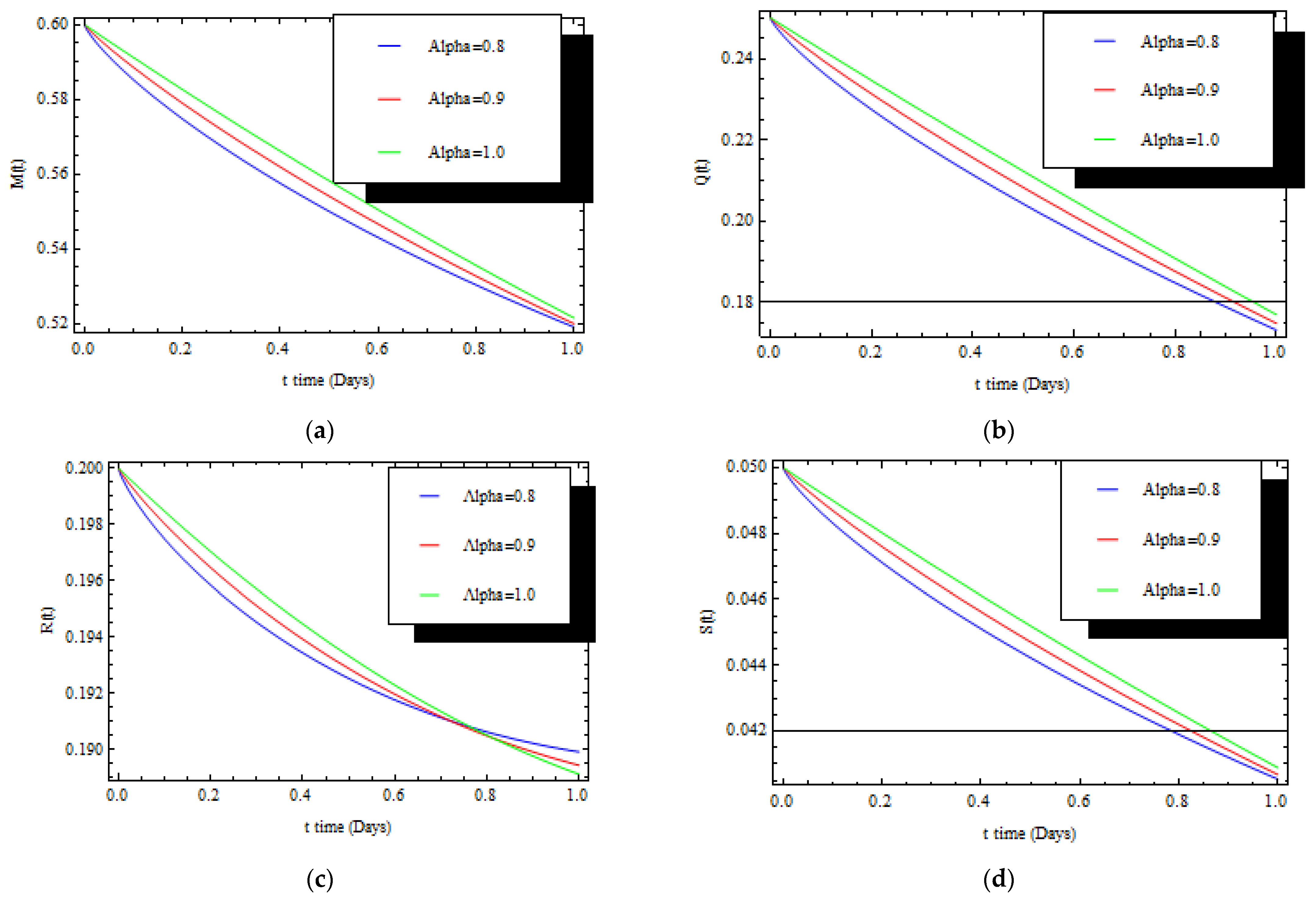
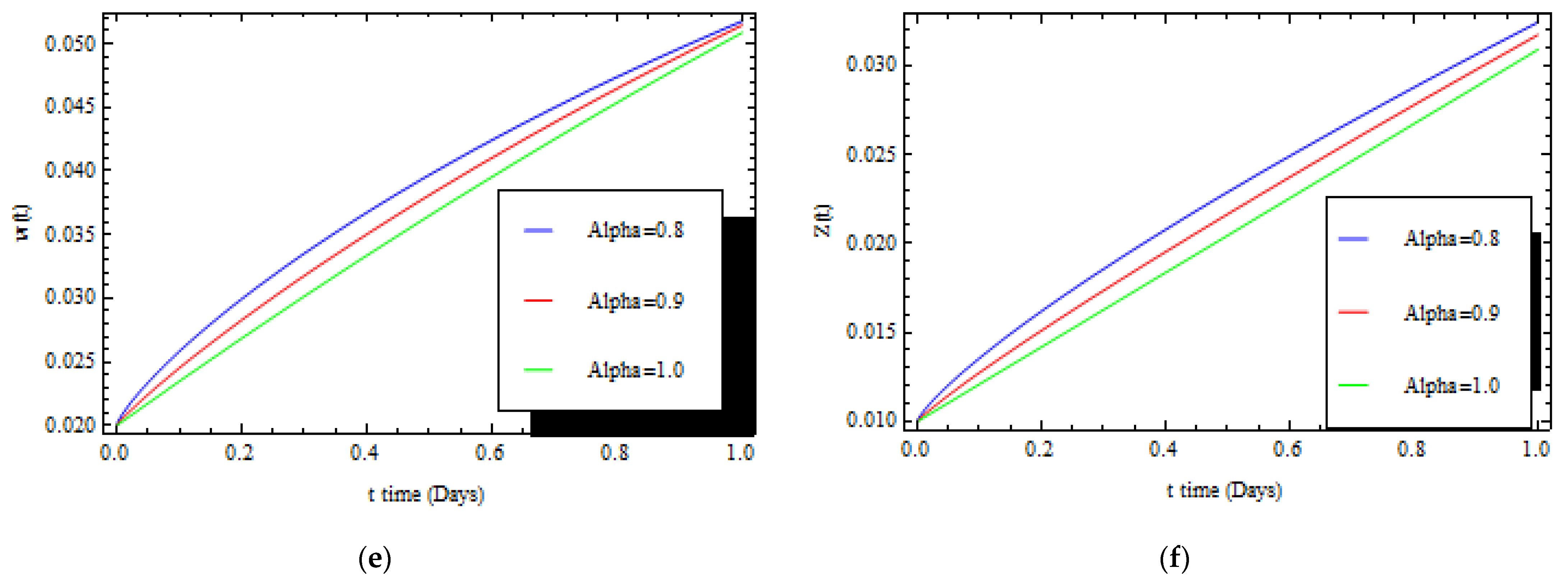
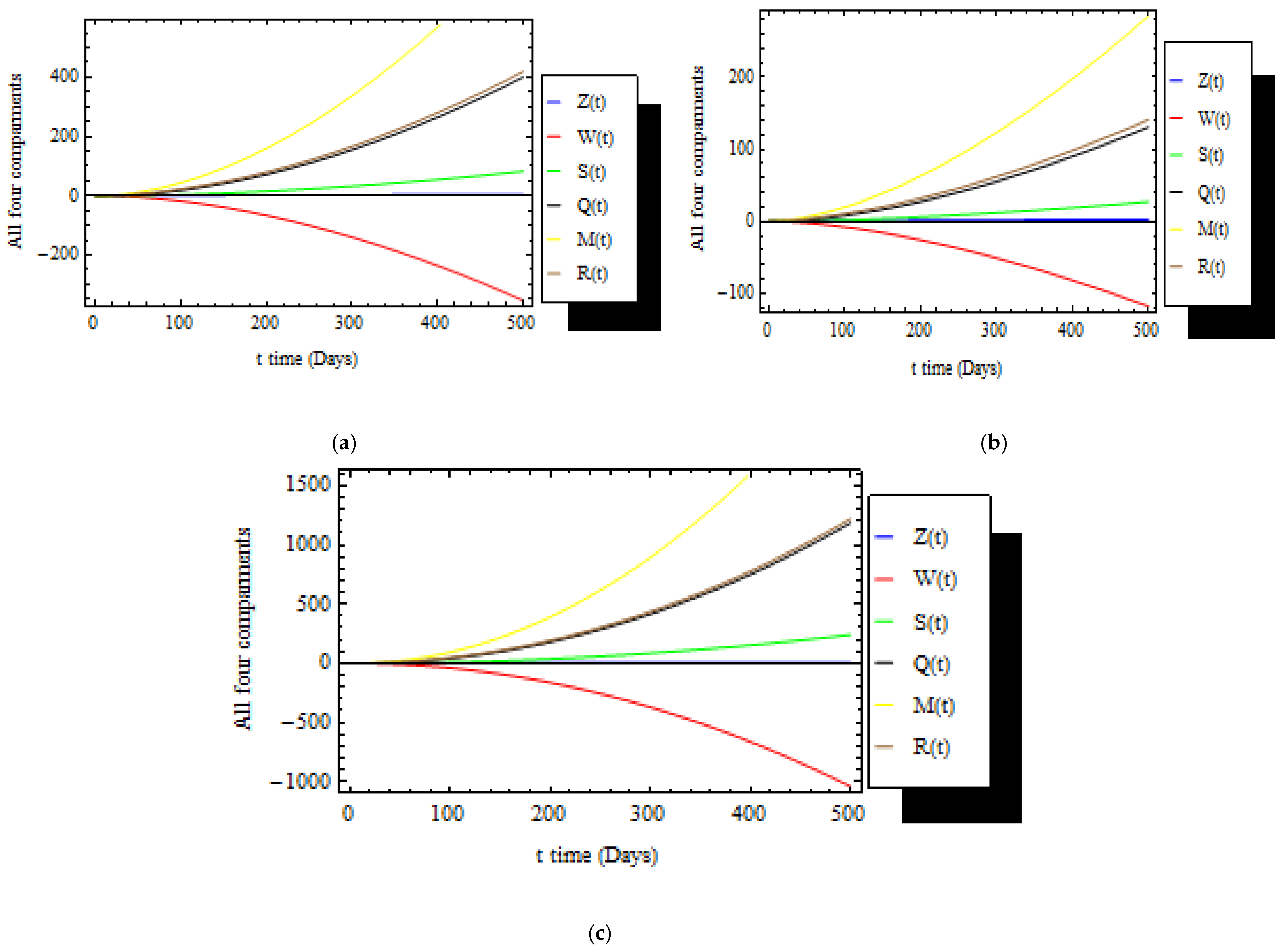
In order to demonstrate the generalization of the NTHAM, we solve the suggested model using other techniques, such as the LHPM [38], and discuss the outcomes. Applying the Laplace transform to both sides of Equation (15), we obtain

$$\begin{array}{l}L[D_t^{\alpha }M] =L[\xi -\beta M R- \beta \psi M S-\eta M {\rm Z}-\delta M],\\ L[D_t^{\alpha }Q]=L[\beta M R+\beta \psi M S+\eta M {\rm Z}\\ -(1-\varphi ) \theta Q-\varphi \vartheta Q-\delta Q],\\ L[D_t^{\alpha }R]=L[(1-\varphi ) \theta Q-\gamma R-\delta R],\\ L[D_t^{\alpha }S]=L[\varphi \vartheta Q-a S-\delta S],\\ L[D_t^{\alpha } \varpi ]=L[\gamma R+a S-\delta \varpi ],\\ L[D_t^{\alpha }{\rm Z}]=L[\sigma R+\epsilon S-k {\rm Z}] .\hspace{1em}\hspace{1em}\hspace{1em}\hspace{1em}0<\alpha \le 1\end{array}$$

(53)

By simplifying, we obtain

$$\begin{array}{l}L[M]-\frac{1}{s}{M}_0-s^{-\alpha }L[\xi -\beta M R- \beta \psi M S-\eta M {\rm Z}-\delta M]=0,\\ L[Q]-\frac{1}{s}{Q}_0-s^{-\alpha }L[\beta M R+\beta \psi M S+\eta M {\rm Z}\\ -(1-\varphi ) \theta Q-\varphi \vartheta Q-\delta Q]=0\\ L[R]-\frac{1}{s}{R}_0-s^{-\alpha }L[(1-\varphi ) \theta Q-\gamma R-\delta R]=0,\\ L[S]-\frac{1}{s}{S}_0-s^{\alpha }L[\varphi \vartheta Q-a S-\delta S]=0,\\ L[\varpi ]-\frac{1}{s}{\varpi }_0-s^{-\alpha }{\displaystyle \sum _{\upsilon =0}^{n-1}{s}^{\alpha -\upsilon -1}{\varpi }_{\tau }^{(\upsilon )}}(0)-s^{\alpha }L[\gamma R+a S-\delta \varpi ]=0,\\ L[{\rm Z}]-\frac{1}{s}{Z}_0-s^{-\alpha }{\displaystyle \sum _{\upsilon =0}^{n-1}{s}^{\alpha -\upsilon -1}{{\rm Z}}_{\tau }^{(\upsilon )}}(0)-s^{\alpha }L[\sigma R+\epsilon S-k {\rm Z} ]=0.\end{array}$$

(54)

Applying the inverse Laplace transform on both sides of Equation (54), we obtain:

$$\begin{array}{l}M(t)=M_0+s^{-\alpha }L[\xi -\beta M R- \beta \psi M S-\eta M {\rm Z}-\delta M],\\ Q(t)=Q_0+s^{-\alpha }L[\beta M R+\beta \psi M S+\eta M {\rm Z}\\ \hspace{1em}\hspace{1em}\hspace{1em}-(1-\varphi ) \theta Q-\varphi \vartheta Q-\delta Q],\\ R(t)=R_0+s^{-\alpha }L[(1-\varphi ) \theta Q-\gamma R-\delta R],\\ S(t)=S_0+s^{\alpha }L[\varphi \vartheta Q-a S-\delta S],\\ \varpi (t)={\varpi }_0+s^{\alpha }L[\gamma R+a S-\delta \varpi ],\\ {\rm Z}(t)=Z_0+s^{\alpha }L[\sigma R+\epsilon S-k {\rm Z} ].\end{array}$$

(55)

Now, applying the classical homotopy perturbation technique, the solution can be expressed as a power series in $p$, as given below.

$$g(x,t)={\displaystyle \sum _{n=0}^{\infty }{p}^n}{g}_n(x,t),$$

(56)

where $p$ is considered a small parameter, $p\in [0,1]$. We can decompose the nonlinear term as:

$$Fg(x,t)={\displaystyle \sum _{n=0}^{\infty }{p}^n}{H}_n(g),$$

(57)

where $H_n$ is a He’s polynomial of $g_0(x,t),g_1(x,t),g_2(x,t),\dots ,g_n(x,t)$, and it can be calculated by the following formula.

$$H_n(g_0(x,t),g_1(x,t),g_2(x,t),\dots ,g_n(x,t))=\frac{1}{n!}\frac{{\partial }^n}{\partial p^n}{[F({\displaystyle \sum _{i=0}^{\infty }{p}^i{g}_i})]}_{p=0} ,n=0,1,2,\dots$$

(58)

Substitution of (56) and (57) into (58) yields:

$$\begin{array}{l}{\displaystyle \sum _{n=0}^{\infty }{p}^n}{M}_n (t)=M_0+L^{-1}[s^{-\alpha }L[\xi -\beta M R- \beta \psi M S-\eta M {\rm Z}-\delta M]]\\ {\displaystyle \sum _{n=0}^{\infty }{p}^n }{Q}_n(t)=Q_0+L^{-1}[s^{-\alpha }L[\beta M R+\beta \psi M S+\eta M {\rm Z}\\ \hspace{1em}\hspace{1em}\hspace{1em}-(1-\varphi ) \theta Q-\varphi \vartheta Q-\delta Q]]\\ {\displaystyle \sum _{n=0}^{\infty }{p}^n }{R}_n(t)=R_0+L^{-1}[s^{-\alpha }L[(1-\varphi ) \theta Q-\gamma R-\delta R]]\\ {\displaystyle \sum _{n=0}^{\infty }{p}^n }{S}_n(t)=S_0+L^{-1}[s^{-\alpha }L[\varphi \vartheta Q-a S-\delta S]]\\ {\displaystyle \sum _{n=0}^{\infty }{p}^n }{\varpi }_n(t)={\omega }_0+L^{-1}[s^{-\alpha }L[\gamma R+a S-\delta \varpi ]]\\ {\displaystyle \sum _{n=0}^{\infty }p}{ }^n {{\rm Z}}_n(t)=Z_0+L^{-1}[s^{-\alpha }L[\sigma R+\epsilon S-k {\rm Z} ]]\end{array}$$

(59)

By equating the coefficients of the corresponding power of $p$ on both sides of Equation (59), the following approximations are obtained:

$$\begin{array}{l}{p}^0:M_0=M(0), p^0:Q_0=Q(0),\\ P^0:R_0=R(0), p^0:S_n=S(0),\\ p^0:{\varpi }_0=\varpi (0), p^0:Z_0=Z(0) ,\end{array}$$

(60)

and

$$\begin{array}{l}p:M_1 =L^{-1}[\frac{1}{s^{\alpha }}L[\xi -\beta M_0 R_0- \beta \psi M_0 S_0-\eta M_0 {{\rm Z}}_0-\delta M_0]]\\ p:Q_1=L^{-1}[\frac{1}{s^{\alpha }}L[\beta M_0 R_0+\beta \psi M_0 S_0+\eta M_0 {{\rm Z}}_0\\ \hspace{1em}\hspace{1em}\hspace{1em}-(1-\varphi ) \theta Q-\varphi \vartheta Q_0-\delta Q_0]]\\ p:R_1=L^{-1}[\frac{1}{s^{\alpha }}L[(1-\varphi ) \theta Q_0-\gamma R_0-\delta R_0]]\\ p:S_1=L^{-1}[\frac{1}{s^{\alpha }}L[\varphi \vartheta Q_0-a S_0-\delta S_0]],\end{array}$$

(61)

$$\begin{array}{l}p:{\varpi }_1=L^{-1}[\frac{1}{s^{\alpha }}L[\gamma R_0+a S_0-\delta {\varpi }_0]]\\ p: {{\rm Z}}_1=L^{-1}[\frac{1}{s^{\alpha }}L[\sigma R_0+\epsilon S_0-k {{\rm Z}}_0 ]].\end{array}$$

(62)

Moreover,

$$\begin{array}{l}{p}^2:M_2 =L^{-1}[\frac{1}{s^{\alpha }}L[\xi -\beta (M_0 R_1+M_1{R}_0)- \beta \psi (M_0{S}_1+M_1 S_0)\\ -\eta (M_0{Z}_1+M_1 {{\rm Z}}_0)-\delta M_1]]\\ p:Q_2=L^{-1}[\frac{1}{s^{\alpha }}L[\beta (M_0{R}_1+M_1 R_0)+\beta \psi ( M_0{S}_1+M_1 S_0)+\eta (M_0 Z_1+M_1{{\rm Z}}_0)\\ \hspace{1em}\hspace{1em}\hspace{1em}-(1-\varphi ) \theta Q_1-\varphi \vartheta Q_1-\delta Q_1]]\\ p^2:R_2=L^{-1}[\frac{1}{s^{\alpha }}L[(1-\varphi ) \theta Q_1-\gamma R_1-\delta R_1]]\\ p^2:S_2=L^{-1}[\frac{1}{s^{\alpha }}L[\varphi \vartheta Q_1-a S_1-\delta S_1]]\\ p^2:{\varpi }_2=L^{-1}[\frac{1}{s^{\alpha }}L[\gamma R_1+a S_1-\delta {\varpi }_1]]\\ p^2: {{\rm Z}}_2=L^{-1}[\frac{1}{s^{\alpha }}L[\sigma R_1+\epsilon S_1-k {{\rm Z}}_1 ]].\end{array}$$

(63)

Then,

$$\begin{array}{l}{M}_2 =\frac{t^{\alpha }}{\Gamma (\alpha +1)}\xi -\frac{t^{2\alpha }}{\Gamma (2\alpha +1)}[\beta (M_0 R_1+M_1{R}_0)\\ + \beta \psi (M_0{S}_1+M_1 S_0)+\eta (M_0{Z}_1+M_1 {{\rm Z}}_0)+\delta M_1]\\ Q_2=\frac{t^{2\alpha }}{\Gamma (2\alpha +1)}[\beta (M_0{R}_1+M_1 R_0)+\beta \psi ( M_0{S}_1+M_1 S_0)\\ +\eta (M_0 Z_1+M_1{{\rm Z}}_0)-(1-\varphi ) \theta Q_1-\varphi \vartheta Q_1-\delta Q_1]\\ R_2=\frac{t^{2\alpha }}{\Gamma (2\alpha +1)}[(1-\varphi ) \theta Q_1-\gamma R_1-\delta R_1]\\ S_2=\frac{t^{2\alpha }}{\Gamma (2\alpha +1)}[\varphi \vartheta Q_1-a S_1-\delta S_1]\\ {\varpi }_2=\frac{t^{2\alpha }}{\Gamma (2\alpha +1)}[\gamma R_1+a S_1-\delta {\varpi }_1]\\ {{\rm Z}}_2=\frac{t^{2\alpha }}{\Gamma (2\alpha +1)}[\sigma R_1+\epsilon S_1-k {{\rm Z}}_1 ].\end{array}$$

(64)

Proceeding in the same manner, the rest of the components $g_n(x,t)$ can be completely obtained, and the series solution is thus entirely determined. The approximate solution $g(x,t)$ is obtained via Equations (46)–(52). This is the same solution obtained via NTHAM and similar to the solution in [32,33] (see Figure 1 and Figure 2).

7. Discussion

This research proposes a new technique called NTHAM for appropriately obtaining novel fractional solutions for the fractional epidemic model (15) based on a mixture of the NT method and HAM. The Mathematica program was used to conduct the calculations. Figure 1 shows various fractional values of $M(t),Q(t),R(t),S(t),\varpi (t),Z(t)$ using initial conditions in [32], and the result is identical to the solution in Ref. [32]. Figure 2 shows all compartments for various fractional orders that correspond to the integer-order solution. Figure 1 and Figure 2 show a comparison of the current solution with fractional solutions produced by q-HASTM [32] and LHPM [38]. In Equations (8) and (9) at u = 1, we have the LT as in Equations (2) and (3). In addition, at s = 1 in Equations (8) and (9), we have the ST as in Equations (5) and (6). Setting $u=1$ in (30) and (31) leads to the solution via the LTHPM in Equation (59) [32]. Additionally, at S = 1, we have the solution reported in the literature via STHAM [33]. It is obvious that the proposed technique in this paper is a generalization of the LT and ST. On the other hand, at alpha = 1, the present solution is the same as the standard solution obtained by Yadav et al. [32]. The NTHAM is characterized by simplicity in producers, does not require strenuous efforts for calculations, and produces high-quality solutions comparable to other techniques.

8. Conclusions

Generic solutions of the FSIRD model are provided by the present technique. It is a combination of the NTM and the HAM. The NTM is considered a generalization of the LTM and STM. Compared with perturbation techniques and non-perturbation methods such as Lyapunov’s artificial small parameter method, the δ-expansion method, and the homotopy perturbation method, the homotopy analysis method has some or all of the following advantages. Firstly, unlike all other analytic techniques, the homotopy analysis method allows substantial freedom to obtain explicit solutions of a given nonlinear problem by means of various base functions. Therefore, we can approximate a nonlinear problem more efficiently by choosing a common group of basic functions. This is because the convergence region and rate of a series are chiefly evaluated via the basic functions used to obtain the explicit solution. The HAM provides us with a family of solution expressions in the auxiliary parameter $ħ$, even if a nonlinear problem has a unique solution. The convergence region and rate of each solution expression among the family might be limited by the auxiliary parameter $ħ$. Thus, the auxiliary parameter gives us an additional way to conveniently adjust and control the convergence region and rate of the solution series. By means of so-called $ħ$-curves, it is easy to find the so-called actual regions of $ħ$ to obtain a convergent solution series. Unlike perturbation techniques, the HAM is independent of any small or large quantities. Furthermore, the proposed technique can be applied to a variety of scientific fields. In the future, we will employ the NTHAM to solve FDES in various aspects of science.

References

1. Breuer, F.; Driesch, V.D. Mathematical Epidemiology; Springer: New York, NY, USA, 2008; p. 415. [Google Scholar]
2. Ma, Z.; Li, J. Dynamic Modeling and Analysis of Epidemics; World Scientific: Singapore, 2009; p. 513. [Google Scholar]
3. Murray, J.D. Mathematical Biology I. An introduction; Springer: New York, NY, USA, 2002; p. 576. [Google Scholar]
4. Kermack, W.O.; McKendrick, A.G. A contribution to the Mathematical Theory of Epidemics. Proc. R. Soc. 1927, 115, 700–721. [Google Scholar]
5. Talaee, M.; Shabibi, M.; Gilani, A.; Rezapour, S. On the existence of solutions for a pointwise defined multi-singular integro-differential equation with integral boundary condition. Adv. Diff. Equ. 2020, 2020, 41. [Google Scholar] [CrossRef]
6. Angstmann, C.N.; Henry, B.N.; McGann, A.V. A fractional order recovery SIR model from a stochastic process. Bull. Math. Biol. 2016, 78, 468–499. [Google Scholar] [CrossRef] [PubMed]
7. Angstmann, C.N.; Henry, B.I.; McGann, A.V. A fractional-order infectivity and recovery SIR model. Fractal Fract. 2017, 1, 11. [Google Scholar] [CrossRef]
8. Kumar, R.; Kumar, S. A new fractional modelling on susceptible-infected-recovered equations with constant vaccination rate. Nonlinear Eng. 2014, 3, 11–19. [Google Scholar] [CrossRef]
9. El-Saka, H.A.A. The fractional-order SIS epidemic model with variable population size. J. Egypt. Math. Soc. 2014, 22, 50–54. [Google Scholar] [CrossRef]
10. Ozalp, N.; Demirrci, E. A fractional order SEIR model with vertical transmission. Math. Comput. Model. 2011, 54, 1–6. [Google Scholar] [CrossRef]
11. AL-Smadi, M.H.; Gumah, G.N. On the homotopy analysis method for fractional SEIR epidemic model. Res. J. Appl. Sci. Eng. Technol. 2014, 7, 3809–3820. [Google Scholar] [CrossRef]
12. Casagrandi, R.; Bolzoni, L.; Levin, S.; Andreasen, V. The SIRC model for influenza A. Math. Biosci. 2006, 200, 152–169. [Google Scholar] [CrossRef]
13. Lin, Q.; Zhao, S.; Gao, D.; Lou, Y.; Yang, S.; Musa, S.S.; Wangb, M.H.; Cai, Y.; Wang, W.; Yang, L.; et al. A conceptual model for the coronavirus disease 2019 (COVID-19) outbreak in Wuhan, China with individual reaction and governmental action. Int. J. Infect. Dis. 2020, 93, 211–216. [Google Scholar] [CrossRef] [PubMed]
14. Jiang, S.; Xia, S.; Ying, T.; Lu, L. A novel coronavirus (2019-nCoV) causing pneumonia-associated respiratory syndrome. Cell. Mol. Immunol. 2020, 17, 554. [Google Scholar] [CrossRef]
15. Gao, W.; Veeresha, P.; Baskonus, H.M.; Prakasha, D.J.; Kumar, P. A new study of unreported cases of 2019-nCOV epidemic outbreaks. Chaos Solitons Fractals 2020, 138, 109929. [Google Scholar] [CrossRef]
16. Liu, Z.; Magal, P.; Seydi, O.; Webb, G. Understanding Unreported Cases in the COVID-19 Epidemic Outbreak in Wuhan, China, and the Importance of Major Public Health Interventions. Biology 2020, 9, 50. [Google Scholar] [CrossRef]
17. Nisar, K.S.; Ahmed, S.; Ullah, A.; Shah, K.; Alrabaiah, H.; Arafan, M. Mathematical analysis of SRID model of COVID-19 with Caputo fractional derivative based on real data. Results Phys. 2021, 21, 103772. [Google Scholar] [CrossRef] [PubMed]
18. Makinde, O.D. Adomian decomposition approach to a SIR epidemic model with constant vaccination strategy. Appl. Math. Comput. 2007, 184, 842–848. [Google Scholar] [CrossRef]
19. Wazwaz, A.M. A new algorithm for calculating Adomain polynomials for nonlinear operators. Appl. Math. Comput. 2000, 111, 53–62. [Google Scholar]
20. He, J.H. Homotopy perturbation technique. Comput. Methods Appl. Mech. Eng. 1999, 178, 257–262. [Google Scholar] [CrossRef]
21. Khan, M.; Gondal, M.A. New modified Laplace decomposition algorithm for Blasius flow equation. Adv. Res. Sci. Comput. 2010, 2, 35–43. [Google Scholar]
22. Khan, Y. An efficient modification of the Laplace decomposition method for nonlinear equations. Int. J. Nonlinear Sci. Numer. Simul. 2009, 10, 1373–1376. [Google Scholar] [CrossRef]
23. Rida, S.Z.; Arafa, A.A.M.; Gaber, Y.A. Solution of the fractional epidemic model by L-ADM. J. Fract. Calc. Appl. 2016, 7, 189–195. [Google Scholar]
24. Liao, S.J. Beyond Perturbation: Introduction to Homotopy Analysis Method; Chapman and Hall/CRC Press: Boca Raton, FL, USA, 2003. [Google Scholar]
25. Liao, S.J. On the homotopy analysis method for nonlinear problems. Appl. Math. Comput. 2004, 147, 499–513. [Google Scholar] [CrossRef]
26. Liao, S.J. Approximate solution technique not depending on small parameters: A special example. Int. J. Nonlinear Mech. 1995, 30, 371–380. [Google Scholar] [CrossRef]
27. El-Tawil, M.A.; Huseen, S.N. The q-homotopy analysis method (q-HAM). Int. J. Appl. Math. Mech. 2012, 8, 51–75. [Google Scholar]
28. El-Tawil, M.A.; Huseen, S.N. On convergence of the q-homotopy analysis method. Int. J. Contemp. Math. Sci. 2013, 8, 481–497. [Google Scholar] [CrossRef]
29. Veeresha, P.; Prakasha, D.G.; Baskonus, H.M. New numerical surfaces to the mathematical model of cancer chemotherapy effect in Caputo fractional derivatives. Chaos Interdiscip. J. Nonlinear Sci. 2019, 29, 013119. [Google Scholar] [CrossRef]
30. Ismail, G.M.; Abedl-Rahim, H.R.; Abdel-Aty, A.; Kharabsheh, R.; Alharbi, W.; Abdel-Aty, M. An analytical solution for fractional oscillator in a resisting medium. Chaos Solitons Fractals 2020, 130, 109395. [Google Scholar] [CrossRef]
31. Ismail, G.M.; Abedl-Rahim, H.R.; Ahmad, H.; Chu, Y.M. Fractional residual power series method for the analytical and approximate studies of fractional physical phenomena. Open Phys. 2020, 18, 799–805. [Google Scholar] [CrossRef]
32. Yadav, S.; Kumar, D.; Singh, G.; Bleanu, D. Analysis and dynamics of fractional order COVID-19 model with memory effect with. Results Phys. 2021, 24, 104017. [Google Scholar] [CrossRef]
33. Bleanu, D.; Mohammad, H.; Rezapour, S. A fractional differential equation model for the COVID-19 transmission by using Caputo-Fabrizio derivative. Adv. Diff. Equ. Phys. 2020, 299, 1–27. [Google Scholar] [CrossRef]
34. Veeresha, P.; Prakasha, D.G.; Baskonus, H.M. Solving smoking epidemic model of fractional order using a modified homotopy analysis transform method. Math. Sci. 2019, 13, 115–128. [Google Scholar] [CrossRef]
35. Baleanu, D.; Aydogn, S.M.; Mohammadi, H.; Rezapour, S. On modelling of epidemic childhood diseases with the Caputo-Fabrizio derivative by using the Laplace Adomian decomposition method. Alex. Eng. J. 2020, 59, 3029–3039. [Google Scholar] [CrossRef]
36. Shah, R.; Khan, H.; Mustafa, S.; Kumam, P.; Arif, M. Analytical Solutions of Fractional-Order Diffusion Equations by Natural Transform Decomposition Method. Entropy 2019, 21, 557. [Google Scholar] [CrossRef]
37. Alotaibi, H.; Abo-Dahab, S.M.; Abdlrahim, H.R.; Kilany, A.A. Fractional calculus of thermoelastic of P-waves reflection under influence of gravity and electromagnetic field. Fractals 2020, 8, 2040037. [Google Scholar] [CrossRef]
38. Singh, J.; Kumar, D.; Kumar, S. New treatment of fractional Fornberg-Whitham equation via Laplace transform. Ain Shams Eng. J. 2013, 4, 557–562. [Google Scholar] [CrossRef]
39. Podlubny, I. Fractional differential equations. In Mathematics in Science and Engineering; Academic Press: San Diego, CA, USA, 1999; p. 198. [Google Scholar]
40. Mittag-Leffler, G. Sur la Nouvelle Fonction Eα(x). C. R. Acad. Sci. Paris 1903, 137, 554–558. [Google Scholar]
41. Caputo, M.; Fabrizio, M. A new definition of fractional derivative without singular kernel Fractional differential equations. Prog. Fract. Diff. Appl. 2015, 2, 73–85. [Google Scholar]
42. Mainardi, F.; Rionero, S.; Ruggeeri, T. On the Initial Value Problem for the Fractional Diffusion-Wave Equation in Waves and Stability Continuous Media; World Scientific: Singapore, 1994; Volume 23, pp. 246–251. [Google Scholar]
43. Wiman, A. Über den Fundamentalsatz in der Teorie der Funktionen. Acta Math. 1905, 29, 191–201. [Google Scholar] [CrossRef]
44. He, J.H. Fractal calculus; its geometrical explanation. Results Phys. 2018, 10, 272–276. [Google Scholar] [CrossRef]
45. Babakhani, A.; Daftardar-Gejj, V. On calculus of local fractional derivative. J. Math. Anal. Appl. 2002, 270, 66–79. [Google Scholar] [CrossRef]
46. Hemeda, A.A.; Eladdad, E.E.; Lairje, A. Local fractional analytical methods for solving wave equations with local fractional derivative. Math. Meth. Appl. Sci. 2018, 41, 2515–2529. [Google Scholar] [CrossRef]
47. Tarasov, V.E. Local fractional derivatives of differentiable functions are integer-order derivatives or zero. Int. J. Appl. Comput. Math. 2016, 2, 195–201. [Google Scholar] [CrossRef]
48. Kolwankar, K.M.; Gangal, A.D. Holder exponents of irregular singles and local fractional derivatives. Pramana J. Phys. 1997, 48, 49–68. [Google Scholar] [CrossRef]
49. Georgiev, S.G. Fractional Dynamic Calculus and Fractional Dynamic Equations on Time Scales; Springer International Publishing: Sofia, Bulgaria, 2018. [Google Scholar]
50. Chen, W.; Liang, Y. New methodologies in fractional and fractal derivatives modeling. Chaos Solitons Fractals 2017, 102, 72–77. [Google Scholar] [CrossRef]
51. Ca, W.; Chen, W.; Xu, W. The fractal derivative wave equation: Application to clinical amplitude/velocity reconstruction imaging. J. Acoust. Soc. Am. 2018, 143, 1559–1566. [Google Scholar] [CrossRef] [PubMed]
52. Atangana, A. Fractal-fractional differentiation and integration: Connecting fractal calculus and fractional calculus to predict complex system. Chaos Solitons Fractals 2017, 102, 396–406. [Google Scholar] [CrossRef]
53. Golmankhaneh, A.K.; Baleanu, D. New derivatives on the fractal subset of real-line. Entropy 2016, 18, 1. [Google Scholar] [CrossRef]
54. Allwright, A.; Atangana, A. Fractal advection-dispersion equation for groundwater transport in fractured aquifers with self-similarities. Eur. Phys. J. Plus 2018, 48, 133. [Google Scholar] [CrossRef]
55. Hu, Z.; Tu, X. A new discrete economic model involving generalized fractal derivative. Adv. Differ. Equ. 2015, 2015, 1–11. [Google Scholar] [CrossRef]
56. Sintunavarat, W.; Turab, A. Mathematical analysis of an extended SEIR model of COVID-19 using the ABC-fractional operator. Math. Comput. Simul. 2022, 198, 65–84. [Google Scholar] [CrossRef]
57. Perez, J.E.S.; Francisco, J.; Aguilar, G.; Baleanu, D.; Tchier, F.; Ragoub, L. Anti-synchronization of chaotic systems using a fractional conformable derivative with power law. Math. Meth. Appl. Sci. 2021, 44, 8286–8301. [Google Scholar] [CrossRef]
58. Rezapour, S.; Souid, M.S.; Bouazza, Z.; Hussain, A.; Etemad, S. On the Fractional Variable Order Thermostat Model: Existence Theory on Cones via Piece-Wise Constant Functions. J. Funct. Space 2022, 2020, 8053620. [Google Scholar] [CrossRef]
59. Watugala, G.K. Sumudu transform-a new integral transform to solve differential equations and control engineering problems. Math. Eng. Ind. 1993, 24, 35–43. [Google Scholar] [CrossRef]
60. Eltayeb, H.; Kılıçman, A. Application of Sumudu Decomposition Method to Solve Nonlinear System of Partial Differential Equations. Abstr. Appl. Anal. 2012, 2012, 1–13. [Google Scholar] [CrossRef]
61. Belgacem, F.B.M.; Karaballi, A.A.; Kalla, S.L. Analytical investigations of the Sumudu transform and applications to integral production equations. Math. Probl. Eng. 2003, 2003, 103–118. [Google Scholar] [CrossRef]
62. Katatbeh, Q.D.; Belgacem, F.B.M. Applications of the Sumudu transform to fractional differential equations. Nonlinear Stud. 2011, 18, 99–112. [Google Scholar]
63. Khan, Z.H.; Khan, W.A. N-transform-properties and applications. NUST. J. Eng. Sci. 2008, 1, 127–133. [Google Scholar]
64. Silambarasan, R.; Belgacem, F.B.M. Applications of the natural transform to Maxwell’s equation. Prog. Electromagn. Res. Symp. Proc. 2011, 899–902. [Google Scholar] [CrossRef]
65. Al-Omari, S.K.Q. On the applications of natural transform. Int. J. Pure Appl. Math. 2013, 85, 729–744. [Google Scholar] [CrossRef]
66. Bulut, H.; Baskonus, H.M.; Belgacem, F.B.M. The analytical solution of some fractional ordinary differential equations by the Sumudu transform method. Abstr. Appl. Anal. 2013, 2013, 1–6. [Google Scholar] [CrossRef]
67. Loonker, D.; Banerji, P.K. Natural transform for distribution and Boehmian spaces. Math. Eng. Sci. Aerosp. 2013, 4, 69–76. [Google Scholar]
68. Loonker, D.; Banerji, P.K. Natural transform and solution of integral equations for distribution spaces. Am. J. Math. Sci. 2013, 3, 65–72. [Google Scholar]
69. Loonker, D.; Banerji, P.K. Applications of natural transform to differential equations. J. Indian Acad. Math. 2013, 35, 151–158. [Google Scholar]
70. Belgacem, F.B.M.; Silambarasan, R.F.M. Theory of natural transform. Math. Eng. Sci. Aerosp. 2012, 3, 99–124. [Google Scholar]
71. Baskonus, H.M.; Bulut, H.; Pandir, Y. The natural transform decomposition method for linear and nonlinear partial differential equations. Math. Eng. Sci. Aerosp. 2014, 5, 111–126. [Google Scholar]
72. Chen, T.; Rui, J.; Wang, Q.; Zhao, Z.; Cui, J.; Yin, L. A mathematical model for simulating the phase-based transmissibility of a novel coronavirus. Infect. Dis. Poverty 2020, 9, 24. [Google Scholar] [CrossRef] [PubMed]
Figure 1. Plots of (a) M ( t ) , (b) Q ( t ) , (c) R ( t ) , (d) S ( t ) , (e) ϖ ( t ) , (f) Ζ ( t ) using specified initial conditions for various fractional values. The result is identical to the solution in [28,38].
Symmetry 14 01695 g001aSymmetry 14 01695 g001b
Figure 2. Plots of all four compartments for various fractional orders, (a) 0.8, (b) 0.9, and (c) 1, corresponding to the integer-order solution.
Symmetry 14 01695 g002
Publisher’s Note: MDPI stays neutral with regard to jurisdictional claims in published maps and institutional affiliations.