An Improved YOLO Algorithm for Fast and Accurate Underwater Object Detection

Abstract

Due to the abundant natural resources of the underwater world, autonomous exploration using underwater robots has become an effective technological tool in recent years. Real-time object detection is critical when employing robots for independent underwater exploration. However, when a robot detects underwater, its computing power is usually limited, which makes it challenging to detect objects effectively. To solve this problem, this study presents a novel algorithm for underwater object detection based on YOLOv4-tiny to achieve better performance with less computational cost. First, a symmetrical bottleneck-type structure is introduced into the YOLOv4-tiny’s backbone network based on dilated convolution and 1 × 1 convolution. It captures contextual information in feature maps with reasonable computational cost and improves the mAP score by 8.74% compared to YOLOv4-tiny. Second, inspired by the convolutional block attention module, a symmetric FPN-Attention module is constructed by integrating the channel-attention module and the spatial-attention module. Features extracted by the backbone network can be fused more efficiently by the symmetric FPN-Attention module, achieving a performance improvement of 8.75% as measured by mAP score compared to YOLOv4-tiny. Finally, this work proposed the YOLO-UOD for underwater object detection through the fusion of the YOLOv4-tiny structure, symmetric FPN-Attention module, symmetric bottleneck-type dilated convolutional layers, and label smoothing training strategy. It can efficiently detect underwater objects in an embedded system environment with limited computing power. Experiments show that the proposed YOLO-UOD outperforms the baseline model on the Brackish underwater dataset, with a detection mAP of 87.88%, 10.5% higher than that of YOLOv4-tiny’s 77.38%, and the detection result exceeds YOLOv5s’s 83.05% and YOLOv5m’s 84.34%. YOLO-UOD is deployed on the embedded system Jetson Nano 2 GB with a detection speed of 9.24 FPS, which shows that it can detect effectively in scenarios with limited computing power.

1. Introduction

The ocean has a tremendous area and volume, and it is rich in natural resources. The utilization of marine resources is bound to attract more and more attention as terrestrial resources are continually exploited and consumed. Underwater robots are commonly used to investigate underwater biological resources [1]. Underwater robots, instead of people, could work in risky environments such as the deep sea and are supplied with cameras or sonar devices for image capture to detect objects [2,3]. Due to its high noise and long wavelength of sound waves, the hydroacoustic signal is not ideal for close-range object detection and recognition for underwater object detection algorithms based on acoustic vision. Light waves, on the other hand, have a tiny wavelength. The images obtained through the visible light band have more details and scene information, are more in line with human observation habits, and are more suitable for real-time performance. Based on this, the focus of this study is on processing underwater photos captured with optical equipment.

Traditional object detection techniques based on manually designed features have a high cost, inability to perform real-time monitoring, and difficulty adapting to complex and changing environments due to cumbersome processing steps and poor generalization in underwater object detection. In recent years, object detection algorithms based on deep learning approaches have been continually attempted and deployed in underwater object detection thanks to the rapid development of deep learning technology. Wang et al. studied deep learning models in underwater object detection and used the you only look once (YOLO) method to effectively detect and identify fish in an underwater environment, achieving real-time detection [4]. Yang et al. established the efficiency of the YOLOv3 algorithm in underwater object detection [5]. They also tested the YOLOv3 method against the faster R-CNN algorithm and discovered that the former performs better. However, they overlooked the limitations of underwater sensing gear, as well as the complicated and changing nature of the underwater illumination environment. Chen et al. [6] proposed a lightweight underwater object detection model based on the principle of YOLOv4-tiny, which reduces the computational complexity of the model by using depthwise separable convolutions instead of traditional convolutions. Still, the large number of 1 × 1 convolutions increases the memory access cost, and the inference performance of the model is only slightly improved. The use of compact convolution kernels to achieve feature generalization is also insufficient.

Although deep-learning-based object detection algorithms can achieve good results in many fields, there are the following problems when they are directly used in underwater robots:

• Insufficient computing power. The human perception limit of video from the camera is 24 frames per second (FPS), so to meet the real-time requirements to some extent, the inferencing speed should be around 10 FPS. However, the high performance of deep neural networks has higher demands on computing resources, which is not well-suited to an environment with underwater robots that are computationally limited.
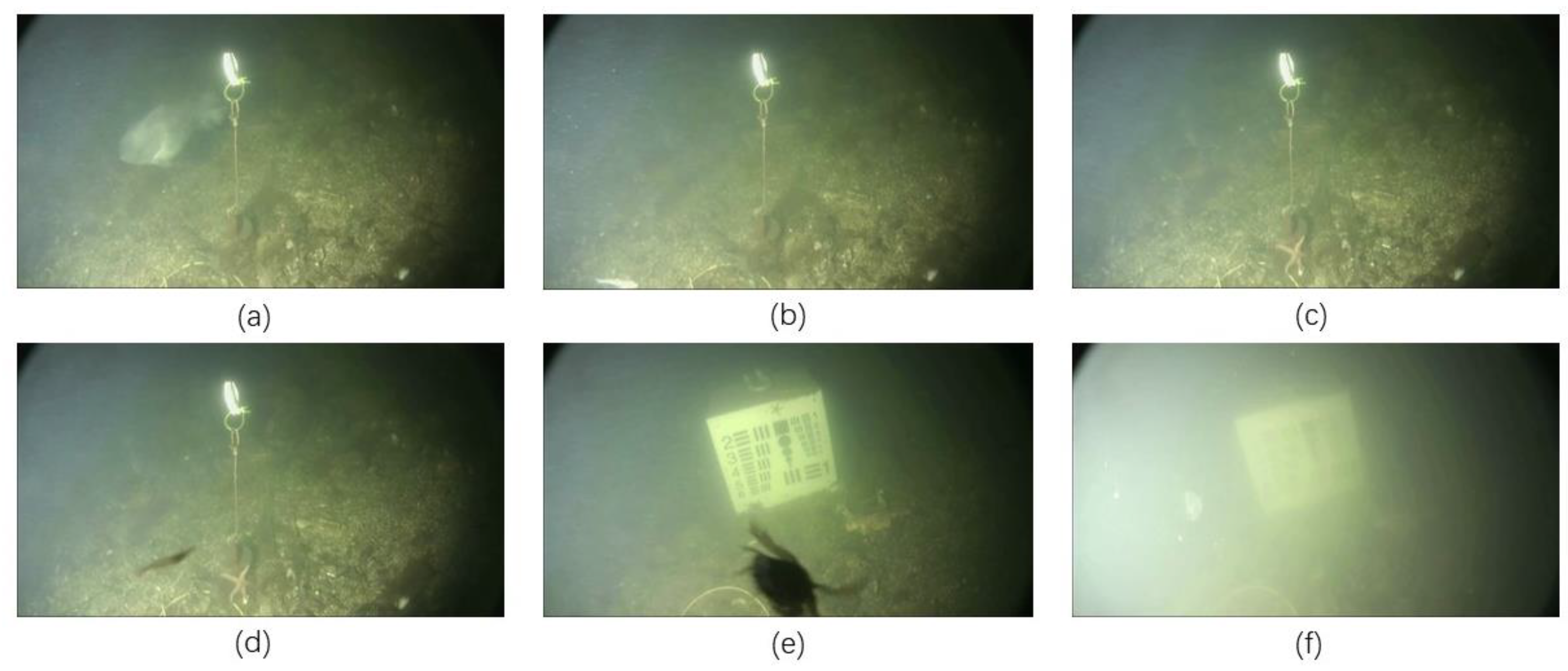
• The underwater image quality is poor. Different from terrestrial imaging, underwater imaging has low-contrast, blurred images, and short visual distance, which lead to problems such as wrong labeling of datasets and easy loss of small objects during detection.

YOLOv4-tiny [7] is an excellent object detector and is faster than YOLOv5 in terms of inference speed, which is more friendly to devices with limited computing power. For this reason, this study chooses YOLOv4-tiny as the baseline model for underwater object detection. However, it is difficult for YOLOv4-tiny to achieve satisfactory detection accuracy. To address the issues above, this study presents a streamlined YOLO structure for underwater object detection and names it YOLO-UOD for convenience. The proposed YOLO-UOD can suit the computational restricted embedded systems and has a better trade-off between speed and accuracy. The following are the primary contributions made in this study:

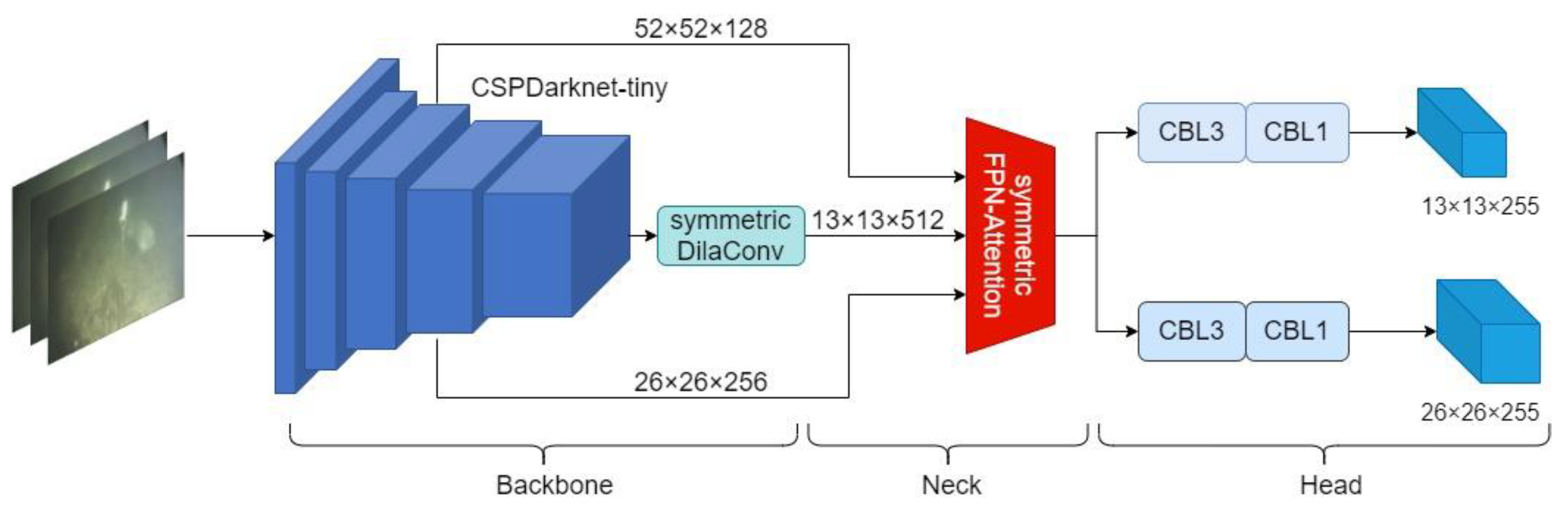
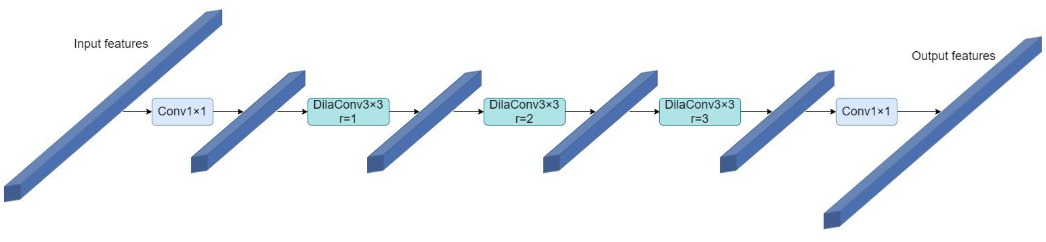
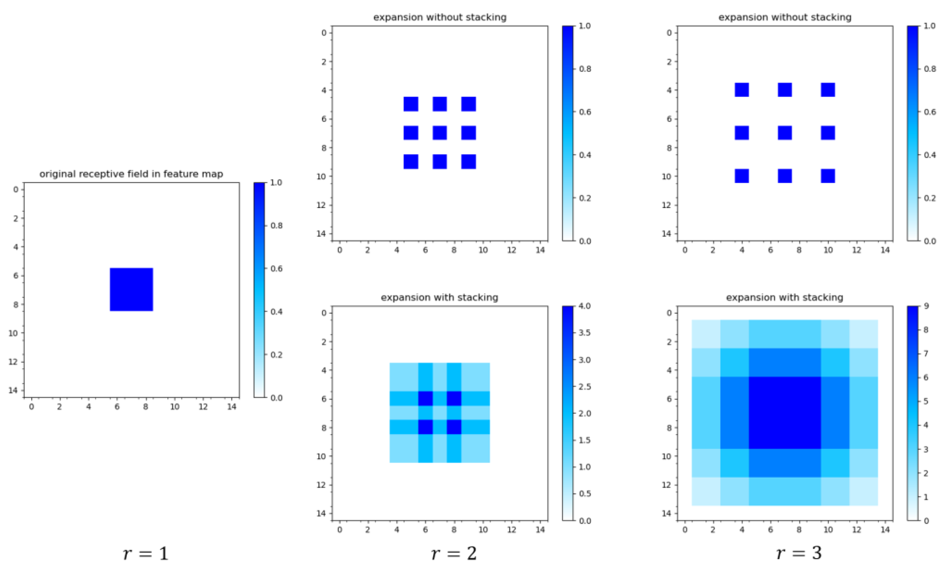
• This study designs a symmetric dilated convolutional module with symmetrical bottlenecks. The proposed symmetric dilated convolutional module is achieved by combining dilated convolutional layers [8] and 1 × 1 convolutional layers in a suitable way, which is able to capture more contextual information with lower computational consumption. The model’s detection mAP score improved by 8.74% by using it to replace the convolution of the last layer in the backbone network of YOLOv4-tiny.
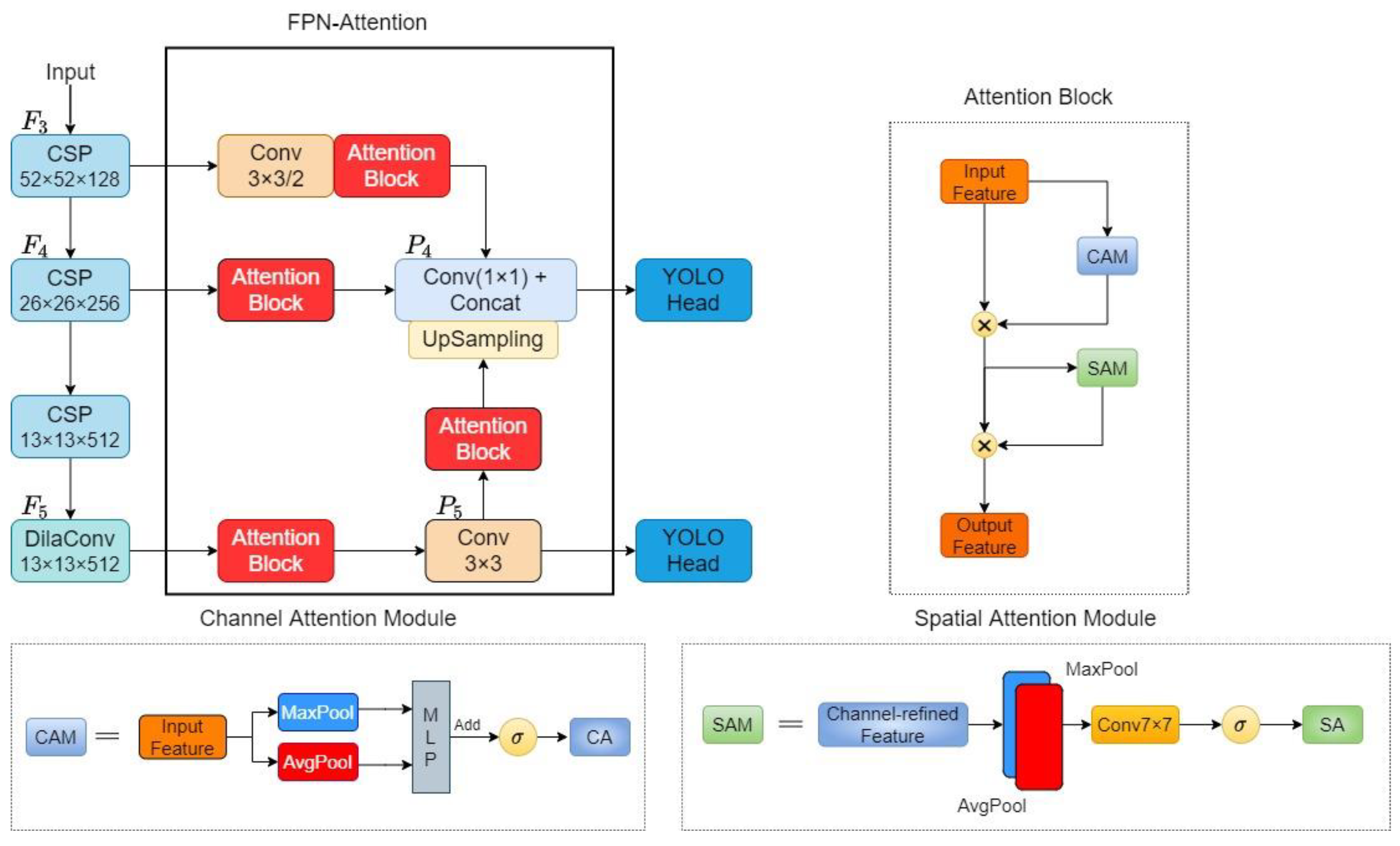
• This study develops a symmetric FPN-Attention module based on the channel-attention module and spatial-attention module in YOLOv4-tiny to increase its detection accuracy while keeping it lightweight. By fusing shallow features with the deeps, the symmetric FPN-Attention module will obtain feature maps with richer semantic information, and a more efficient feature fusion can be achieved through the attention module. The mAP score of YOLOv4-tiny can be improved by 8.75% when the symmetric FPN-Attention module is used. In addition, label smoothing is used during training to suppress the potential labeling mistakes to some extent and improve the model’s generalization for underwater object data.
• Experimental results on the Brackish underwater dataset [9] show that the proposed YOLO-UOD has higher detection performance in underwater object detection with 87.88% mAP, which surpasses YOLOv4-tiny’s 77.38%, YOLOv5s’s 83.05%, and YOLOv5m’s 84.34%. Besides, the proposed detector runs at about 9.24 FPS on Jetson Nana 2 GB, which is faster than YOLOv5s at 8.38 FPS and YOLOv5m at 4.11 FPS. The results show that YOLO-UOD has a better speed/accuracy trade-off underwater.

The rest of this work is arranged in the following manner: A brief overview of recent relevant work is presented in Section 2, which focuses on the YOLOv4-tiny architecture and its benefits and drawbacks. The implementation specifics of the YOLO-UOD algorithm are detailed in Section 3. Section 4 presents relevant experimental information, including results, while Section 5 concludes.

2. Related Work

This section provides some background information on the proposed underwater object detection algorithm, including the basic framework of object detection, the YOLOv4-tiny algorithm framework, and the attention module.

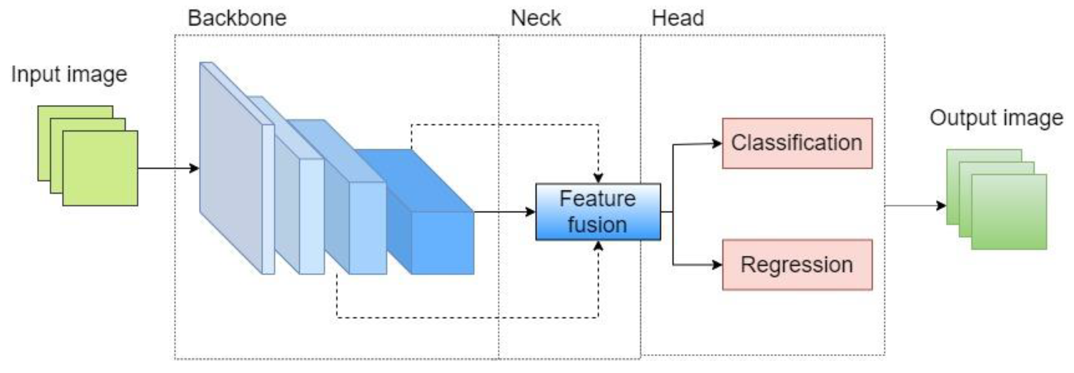
2.1. Basic Framework for Object Detection

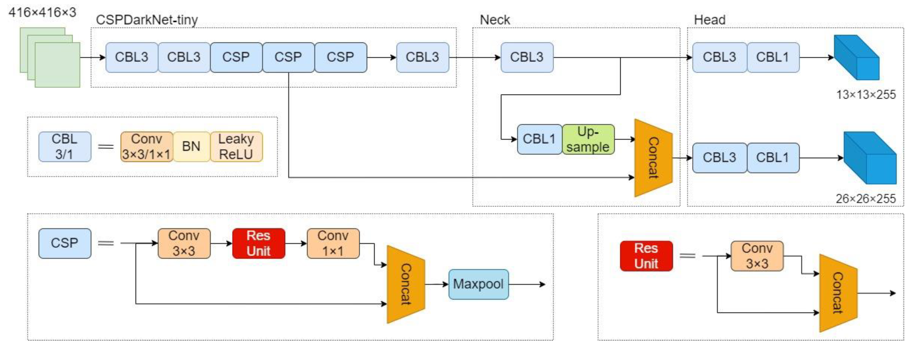
Object detection is a downstream problem in computer vision that has a wide range of practical applications [10,11,12,13]. Deep-learning-based object detection algorithms can be divided into two categories based on whether or not a proposal generation stage is present: two-stage object detection algorithms such as R-CNN (regions with convolutional neural network features) [14], Fast-RCNN [15], Faster-RCNN [16]; and one-stage object detection algorithms such as SSD (single shot multibox detector) [17], RetinaNet [18], FCOS (fully convolutional one-stage object detection) [19], and YOLO [20]. A standard component of the convolutional neural network (CNN)-based object detector consists of a backbone for feature extraction, a neck for feature fusion, and a head prediction module. Figure 1 shows the framework of a CNN-based object detector.

Because of the extra step for the region proposal, the two-stage object detector is better than the one-stage object detector in terms of detection precision. However, it also adds to the computation time, which is not favorable for real-time detection of the model. As a result, the one-stage object detection method YOLO is the topic of this research.

2.2. YOLOv4-Tiny

The YOLO one-stage object detection algorithm eliminates the region proposal branch, allowing for faster online inference. Although the early YOLO [20,21] algorithms have a faster detection speed, their detection precision is not adequate. YOLOv3 [22] is the first to attain a superior speed/accuracy trade-off. Furthermore, Bochkovskiy et al. proposed YOLOv4 [23] by designing a new feature extraction network, CSPDarkNet53, based on the cross-local connectivity structure of CSPNet [24] to generate richer gradient combinations while reducing the required computing effort. However, YOLOv4 generates a significant memory footprint, making it difficult to adapt to inference requirements on computationally restricted systems. Wang et al. scaled YOLOv4 and designed YOLOv4-tiny based on it [7]. Figure 2 depicts the overall structure of the YOLOv4-tiny model.

As shown in Figure 2, the YOLOv4-tiny backbone uses CSPDarkNet-tiny, which consists primarily of cross-stage partial connections (CSP) and CBL components, with CBL being a typical convolution featuring batch normalization (BN) and Leaky ReLU (rectified linear unit) activation functions. As a significant part of the feature extraction network, the CSP component uses a cross-local interconnection topology. After a layer of feature mapping, the input is divided into two channels, one of which leads directly to the end of the connection stage, and the other branch enters the dense layer after a series of affine transformations. It is spliced with the previous branch through a cross-regional connection, as shown in the diagram. In this approach, when updating the weights, it is feasible to avoid learning a large number of repetitive gradients again, produce a richer mix of gradients, and lower the computing cost to a degree. Notably, the BN layer following the standard convolution allows each layer in the CNN to maintain the same distribution of input, which can speed up the convergence of the model. Suppose that $x_i$ is the $i-th$ sample, and there are $m$ samples in a mini-batch $B=\left\{x_{i\dots m}\right\}$. The BN can be represented by Equation (1).

$${\widehat{x}}_i=\frac{x_i-u_B}{\sqrt{{\sigma }_B^2+ϵ}}, y_i=\gamma {\widehat{x}}_i+\beta$$

(1)

where ${\widehat{x}}_i$ is the normalized tensor for each input $x_i$, $y_i$ is the output obtained after scaling and offsetting ${\widehat{x}}_i$, and $ϵ$ is the smoothing term that assures numerical stability by stopping a division by a zero value that is usually set as 1 × 10⁻⁵. $u_B$ and ${\sigma }_B^2$ denote the batch mean and variance, respectively, as shown in Equation (2). The scaling factor $\gamma$ and the offset factor $\beta$ are trainable parameters.

$${\mu }_B=\frac{1}{m}{{\displaystyle \sum }}_{i=1}^m{x}_i, {\sigma }_B^2=\frac{1}{m}{{\displaystyle \sum }}_{i=1}^m{\left(x_i-u_B^2\right)}^2$$

(2)

After the backbone network extracts features, YOLOv4-tiny uses the feature fusion network (FPN) [25] structure for the multi-scale fusion of the extracted features, resulting in the classification and regression of feature maps at various scales in the network prediction layer. Compared with YOLOv4, on the CSP component, YOLOv4-tiny deletes a large number of 1 × 1 convolutions to achieve the highest possible parameter utilization. It utilizes a maximum pooling layer of size 2 × 2 with step size of 2 for down-sampling to reduce the number of parameters and introduce nonlinearities. However, the CSP components of the same feature map size are not stacked repeatedly in YOLOv4-tiny, which reduces the computational complexity of the model and the number of parameters to some extent. However, the model’s ability to extract features from the data is also reduced, making it difficult to obtain an adequate representation of the input space or data.

2.3. Attention Module

The attention module was developed as a result of research into human vision and may also be considered as a resource allocation approach for computational resources. In computer vision, one important task is to opt for a more robust feature representation that captures the most critical attributes of the object of interest in a given task, thus improving the model’s ability to represent the features. Hu et al. proposed the squeeze-and-excitation (SE) module [26], which computes channel attention scores through global average pooling and weights the feature maps, eventually achieving state-of-the-art (SOTA) performance on multiple datasets and tasks. The SE module demonstrated that previous architectures are unable to adequately model feature dependencies in terms of channels. The SE module, however, does not make use of spatial data. Woo et al. introduced a new attention module [27] that combined spatial and channel attention to attain SOTA performance on PASCAL VOC2007. Intending to capture local cross-channel interactions, Wang et al. investigated a one-dimensional convolution with adaptive kernel size to replace the fully connected layer in channel attention based on the SE module and proposed a more efficient and less computationally complex attention mechanism [28].

The neck feature layer is located after the feature extraction network in the object detector to fuse feature maps of various scales to generate a multi-scale visual representation. The semantic information in the feature maps is continuously increased during the down-sampling process in the convolutional neural network, which is necessarily accompanied by the loss of location information. Feature representations of various scales correlate with feature maps of various depths. Shallow feature maps have higher resolution and more location information, but they lack effective feature representation. Deep feature maps have a lower resolution and a drastic reduction of location information, but they include more semantic information. As a result, the accuracy of the classifier’s final prediction results is dependent on how efficiently the fused shallow and deep feature maps are connected to produce a feature map that contains sufficient semantic and location information. In this paper, an attention module is added to the feature fusion layer to increase the model inference effect by enhancing the features extracted by the backbone network.

3. Improved YOLO Algorithm

This section presents the proposed YOLO-UOD method. Figure 3 shows the overall flow chart of the YOLO-UOD, which consists of three components: backbone network, neck network, and head network. As shown in Figure 3, YOLO-UOD inherits the backbone network of YOLOv4-tiny, and the difference is that the proposed method substitutes the original convolutional layers with a symmetric dilated convolutional module for a broader receptive field. Following that, the proposed symmetric FPN-Attention module replaces the original neck of YOLOv4-tiny to improve the detection ability of the model. Finally, label smoothing is used in the training stage to reduce the detrimental impact of data labeling mistakes on model performance and keep the YOLOv4-tiny’s head network unchanged.

3.1. Symmetric Dilated Convolutional Module

An object cannot exist alone in the real world; it must have a relationship with the surrounding environment or objects, often known as the image’s contextual information. It is believed that the features of the object will have similarities with the noise underwater to some extent. Therefore, this work introduces a dilated convolution in the last layer of the original feature extraction network of YOLOv4-tiny to expand the receptive field, allowing the object detector to make full use of the contextual information in the image. Let the size of the convolution kernel be $k$, and the expansion factor be $r$. The actual size $k_d$ of the dilated convolution can be expressed as Equation (3).

$$k_d=k+\left(k-1\right)·\left(r-1\right)$$

(3)

It can be found that when $r=1$, the dilated convolution is equivalent to the standard convolution. However, the effect of expanding the receptive field is achieved by injecting voids into the convolution kernel during the convolution process. This will lead to inevitable loss, to some extent, in image details and a loss of continuity and integrity among the data (as shown in Figure 4), especially in the deep feature maps, which will have disastrous effects. Therefore, multiple layers of the dilated convolution are stacked with different expansion factors (as shown in Figure 4) and designed in a symmetric structure that can effectively alleviate the detail loss during the dilated convolution. Figure 4 shows the dilated convolution field size plots with different expansion factors.

The receptive field size of the dilated convolution with different expansion coefficients without stacking grows with the expansion coefficient, as seen in the upper portion of Figure 4, but the loss of information also increases. It is not difficult to see that after stacking the dilated convolutions with expansion coefficients of 1, 2, and 3, the size of the receptive field increases from 3 × 3 to 7 × 7 and finally reaches 13 × 13, successfully using all of the information in the receptive field.

When stacking the dilated convolution, for the input feature map whose shape is $insize$, the output’s shape $outsize$ can be obtained by Equation (4).

$$outsize=\frac{insize+2p-k-\left(k-1\right)\left(r-1\right)}{s}+1$$

(4)

where $p$ denotes the filling of the feature map, and $s$ represents the step size of the convolution. From Expression (4), it can be seen that when $s=1$and $k=3$, it is necessary to have $p=r$ to keep the size of the feature map unchanged during the dilated convolution. Therefore, this study will use the values 1, 2, and 3 for $p$. Furthermore, the 1 × 1 convolution is implemented to lower dimensionality first and then raise it, generating a symmetric bottleneck-type structure that can alleviate overfitting and reduce the number of parameters in the process of dilated convolution stacking. The structure of the symmetric dilated convolutional module is shown in Figure 5.

3.2. Symmetric FPN-Attention Module

The FPN network is used in the neck module of YOLOv4-tiny. The deep feature map with robust semantic information obtained by multiple down-sampling is first aligned by 1 × 1 convolution, then fused with the shallow feature map with weak semantic information by up-sampling, resulting in a feature map with richer semantic information. However, as the down-sampling multiplicity increases steadily, the spatial location information of the feature map is gradually lost, affecting the object detector’s performance.

Based on this, the model’s neck connection layer is redesigned, as shown in Figure 6. First, the feature map $F_5$ is obtained in the backbone network after five rounds of down-sampling and the symmetric dilated convolution module, after which the attention module is centrally allocated the computational resources. Second, the output of the weighted feature map is divided into two paths after a standard 3 × 3 convolution. One path is fed to the head layer for feature classification and regression for the detection of large objects. The other path is passed to another attention module and aligned with the feature map $F_4$ in the spatial dimension by up-sampling, and then aligned with the channel dimension by 1 × 1 convolution. Finally, the two are stitched together by channel. Moreover, the proposed method concatenates the feature maps $F_3$ and $F_4$; these have been down-sampled three times to improve the model’s ability to detect small objects, and they construct a top and symmetrical bottom architecture. $F_3$ is down-sampled at first for feature alignment by 3 × 3 convolution with a step size of 2. Then, it is aligned by 1 × 1 convolution for channel alignment, and the same attention module is used in the process.

Let $DilaCon{v}_r(·)$ denote the dilated convolution with expansion coefficient $r$, $A(·)$ denote the attention mechanism, $Up(·)$ denote the up-sampling, and $Con{v}_{k/s}$ represent a convolution with kernel size of $k\times k$ and stride of $s$. The $s$ is set to 1 by default. $P_4$ and $P_5$ respectively denote the aggregated feature maps corresponding to different levels of down-sampling. Then, the process of feature fusion using the above can be represented by Expressions (5) and (6).

$$P_4=A[Con{v}_3\left(F_4\right)+Con{v}_1\left(Up\left(P_5\right)\right)\left]+Con{v}_1\right[A\left(Con{v}_{3/2}\left(F_3\right)\right)]$$

(5)

$$P_5=DilaCon{v}_{1,2,3}\left(F_5\right)$$

(6)

The convolutional block attention module (CBAM) [27], which comprises the channel-attention module (CAM) and the spatial-attention module (SAM), as shown in Figure 6, is used as a concrete implementation of the attention module. The input features $F$ obtained from affine translation will first travel through the average pooling layer and the maximum pooling layer in the CAM. The average pooling layer is considered to learn the range of objects effectively. In contrast, the maximum pooling layer can collect salient features of objects to aggregate spatial information, after which the shared weights obtained from the multilayer perceptron (MLP) are summed element by element. The final channel attention score map $M_C\left(F\right)$ is obtained after sigmoid activation, and $F_{CA}$ represents the feature map after the channel attention module, which is obtained by multiplying the input feature map with $M_C\left(F\right)$ element by element. The expression is shown in Equation (7).

$$\begin{array}{c}{F}_{CA}=M_C\left(F\right)\otimes F\\ =\sigma \left(MLP\right(\mathit{AvgPool}\left(F\right))+MLP(\mathit{MaxPool}\left(F\right)\left)\right)\otimes F\\ =\sigma \left(W_1\right(W_0\left(F_{\mathit{avg}}^C\right))+W_1(W_0\left(F_{\mathit{max}}^C\right)\left)\right)\otimes F\end{array}$$

(7)

where $\otimes$ denotes element-by-element multiplication, $W_0\in {ℝ}^{C/\gamma \times C}$ and $W_1\in {ℝ}^{C\times C/\gamma }$ are the weight matrix of the MLP, $\sigma (·)$ denotes the sigmoid function, and $\gamma$ denotes the dimensional scaling factor. $F_{avg}^C$ and $F_{max}^C$ represent the mean and maximum value on each feature map by channel, respectively.

After obtaining $F_{CA}$ through the channel attention module, it is mapped to the spatial attention module as the input features. As can be seen from the right bottom of Figure 6, the feature map is first subjected to maximum pooling and average pooling operations along the channel axis. Following that, the two channels are combined by a 7 × 7 convolutional layer. The spatial feature score map $M_S\left(F\right)$ is obtained through the sigmoid function. $F_{SA}$ represents the feature map after the spatial attention module, which is obtained by multiplying the input feature map with $M_S\left(F\right)$ element by element, and the expression is shown in Equation (8).

$$\begin{array}{c}{F}_{SA}=M_S\left(F\right)\otimes F_{CA}\\ =\sigma \left({\mathit{Conv}}_{7\times 7}\right(\left[\mathit{AvgPool}\right(F);\mathit{MaxPool}(F\left)\right]\left)\right)\otimes F_{CA}\\ =\sigma \left({\mathit{Conv}}_{7\times 7}\right([F_{\mathit{avg}}^S;F_{\mathit{max}}^S]\left)\right)\otimes F_{CA}\end{array}$$

(8)

where $F_{avg}^S$ and $F_{max}^S$ represent the mean and maximum value of feature map along the channel, respectively.

3.3. Label Smoothing

When optical image detection is performed underwater, it frequently encounters issues such as flowing water, light absorption, and scattering, causing low contrast and uneven color distribution in the acquired optical images. As a result of the inaccuracy of manual labeling, noise is invariably introduced in supervised learning. Therefore, this research uses label smoothing [29] to alleviate the labeling error problem in the classification problem. For the multiclassification problem, let $z_i$ denote the predicted probability distribution of class $i$, $q_i$ denotes the confidence score of the current data corresponding to class $i$, and $K$ denotes the number of labels, whose expression is shown in Equation (9).

$$q_i=\sigma \left(z_i\right)=\frac{\exp \left(z_i\right)}{{{\displaystyle \sum }}_{j=1}^k\exp \left(z_j\right)}$$

(9)

When utilizing cross-entropy loss to calculate the probability of each category in multiclassification problems, the category labels are frequently stored in one-hot form, which causes the model to reward successful classification the most and penalize erroneous classification the most. When the training data is not guaranteed to be accurate, it also leads to the problem of overfitting the model. The cross-entropy loss function $L_{CE}$ is shown in Equation (10).

$$\begin{array}{c}{L}_{CE}(p,q)=-{\displaystyle {{\displaystyle \sum }}_{i=1}^K}{p}_i\log q_i=-\log p_y\\ =-z_y+\log ({{\displaystyle \sum }}_{j=1}^K\exp (z_j))\end{array}$$

(10)

where $p_i$ denotes the true probability distribution of the $i-\mathrm{th}$ category expressed as a one-hot vector, $y$ denotes the actual label of the image, $p_i=1$ when and only when $i=y$, and $p_i=0$ in the rest of the cases. The result of the cross-entropy loss function is 0 when the classification is correct and infinity when incorrect. It will cause the model to learn in the direction of the largest difference between correct and incorrect labels, which may lead to overfitting in the case of insufficient data or inaccurate data labeling. To solve this problem, using soft one-hot noise to minimize the weight of the real sample label categories in the loss function computation can result in constant overfitting. After label smoothing, $p_i^{*}$ can be expressed as Equation (11).

$$p_i^{*}=p_i\left(1-\alpha \right)+\alpha /K=\{\begin{array}{cc}\hfill 1-\alpha , & i=y\hfill \\ \hfill \alpha /K, & otherwise\hfill \end{array}$$

(11)

where $\alpha$ is the hyperparameter that controls the introduced noise. The cross-entropy loss $L_{CE}{ }^{*}$, at this point, can be expressed as Equation (12).

$$\begin{gathered} L_{CE}{(p,q)}^{*}=-{{\displaystyle \sum }}_{i=1}^K{p}_i^{*}\log q_i \\ =-\left(1-\alpha +\alpha /K\right)\log q_i-\alpha /K{\displaystyle \sum }_{i\ne y}\log q_i \end{gathered}$$

(12)

At this point, the ideal solution $z_i^{*}$ can be represented as Equation (13).

$$z_i^{*}=\{\begin{array}{cc}\hfill \log \left(\left(k-1\right)\left(1-\alpha \right)\right)/\left(\alpha +\epsilon \right),& i=y\hfill \\ \hfill \epsilon ,& otherwise\hfill \end{array}$$

(13)

where $\epsilon$ can be expressed as any real number. Regularization reduces the output difference between the correct and incorrect classes, which helps to prevent the network from overfitting and improves the model’s robustness.

4. Experiments

The proposed YOLO-UOD is quantitatively trained and evaluated on the Brackish underwater dataset in this section, and ablation experiments are undertaken to validate the effectiveness of the proposed improvements, with the experimental details and results described.

4.1. Experimental Environment and Configuration

4.1.1. Underwater Image Dataset

This work uses the Brackish underwater dataset [9] as the training dataset and test dataset for the model. The Brackish underwater dataset contains 10,995 original images of underwater objects and their accompanying annotation files, with a total of six object types, as shown in Figure 7, namely big fish, small fish, starfish, shrimp, crab, and jellyfish. The dataset is chosen at random in an 8:1:1 ratio and separated into training, validation, and test sets, accordingly. The training set has 8905 photos for training the model, the validation set contains 990 images for evaluating the model during the training process, and the test set, which contains 1100 images, is used to assess the model’s actual performance.

An effective training data set is one of the most important ways to increase the detection accuracy of a deep-convolutional-network-based object detector. When object detection is done in an underwater environment, the imaging technique is affected by light absorption and scattering (Figure 7). The underwater image appears blue-green in hue due to the wavelength dependence of visible light propagation in the water body, while light scattering by impurity particles in the water generates blurred image details as well as surface haze. As a response, this work performs operations such as image improvement (e.g., contrast stretching and color gamut transformation) on the original image before feeding it into the network for training. Mosaic enhancement is not used throughout the training procedure because of its volatility during the process.

4.1.2. Evaluation Metrics

A qualified object detector is able to classify and localize objects of interest in an image or video with a sufficiently high confidence level [30]. When evaluating object detectors, precision refers to the model’s capacity to correctly anticipate the object of interest, while recall refers to the model’s ability to locate all objects of interest. In Equations (14) and (15), the precision and recall expressions are shown, respectively.

$$\mathrm{precision} =\frac{\mathrm{TP}}{all detections}=\frac{\mathrm{TP}}{\mathrm{TP} + \mathrm{FP}}$$

(14)

$$\mathrm{recall}=\frac{\mathrm{TP}}{all ground-truths}=\frac{\mathrm{TP}}{\mathrm{TP} + \mathrm{FN}}$$

(15)

where TP denotes the number of correctly predicted positive samples, FP denotes the number of negative samples predicted as positive samples, and FN denotes the number of positive samples predicted as negative samples. Their relationships can be represented in

Table 1. Classification confusion matrix.

	Prediction	Positive	Negative
Ground Truth
Positive		TP	FN
Negative		FP	TN

.

In practical detection tasks, both accuracy and recall are usually required to maintain a superior score. However, accuracy × recall is often not monotonic, but shows a sawtooth shape. Average precision (AP) is a measure of the area under the precision × recall curve, which summarizes an equilibrium state of precision and recall determined by the confidence level of the prediction bounding box to represent the accuracy of the model concerning a certain category. This study uses mean average precision (mAP) to denote the average of all classes, and $N$ to denote the total number of discovered object classes. The expression for mAP can be seen in Equation (16).

$$m\mathrm{AP} =\frac{1}{N}{{\displaystyle \sum }}_{i=1}^N{{\displaystyle \int }}_0^{1}P dR$$

(16)

where $P$ denotes the precision value, and $R$ denotes the recall value.

4.1.3. Experimental Environment

The experimental software environment is Ubuntu 20.04, CUDA version 11.3, cuDNN version 8.2.0.53, PyTorch 1.8.1 deep learning framework, and the Python 3.8 programming environment. The Nvidia RTX3090 GPU and the i9-10920X are used as the hardware environment to train the model. Transfer learning is employed to tackle the problem of limited sample size and speed up network convergence by using the ImageNet pre-trained model as the backbone network’s initialization weights and then training the model on the Brackish underwater dataset. In the experimental process, the stochastic gradient descent (SGD) optimizer with a momentum of 0.9 is utilized. The batch size is set to 64, the starting learning rate is 2 × 10⁻³, and the learning rate decrease strategy is StepLR with 100 epochs throughout the training. The warm-up is adopted within the first five epochs of the training to accomplish the initial learning rate, which mitigates the early overfitting phenomena of the model to the mini-batch in the beginning stage. After that, at the 30th, 60th, and 90th epochs, the learning rate is reduced to one-fifth of the previous rate.

This work tabulated the testing/training execution times for YOLO-UOD and other contrast algorithms on the server, as shown in

Table 2. Training/testing execution times of the algorithms on the server.

Model	Training Time (Hours)	Testing Time (Image/ms)
RetinaNet	3.6	19.70
YOLOv3	3.9	9.56
YOLOv4-tiny	2.1	5.35
YOLOv5s	1.7	8.85
YOLOv5m	2.3	12.35
YOLO-UOD	2.1	6.18

.

4.2. Comparison and Analysis of Experimental Results

In order to facilitate batch training, the size of the input image is fixed to 416 × 416 when training the model. Following the training, the validation dataset, which uses the dataset partitioning described in Section 4.1.1, is fed into the trained network.

4.2.1. Ablation Experiments

Several ablation experiments are conducted to show the superiority of the proposed structure, and the results in mAP are reported in

Table 3. Ablation experiment.

DilaConv	Symmetric FPN-Attention	Label Smoothing	Brackish
			77.38
√			86.12
	√		86.13
√	√		87.37
√	√	√	87.88

. The check box in Table 3 indicates that this module is used. The DilaConv denotes the symmetric dilated convolutional module. This table shows that the original YOLOv4-tiny has an mAP score of 77.38% on the Brackish underwater dataset. First, the model achieves 86.12% with the DilaConv module, which is 8.74% higher than YOLOv4-tiny’s score, indicating that the DilaConv module is able to capture global information effectively and preserve semantic information. Second, by combining with the symmetric FPN-Attention module, this model achieves a score of 86.13%, which is 8.75% higher than YOLOv4-tiny’s score, meaning that the symmetric FPN-Attention module makes the computational resources allocated by the model more focused on representing valuable features. Following that, the performance of the network reaches 87.37% by combining the DilaConv module and the symmetric FPN-Attention module. The final score achieves 87.88% by using the label smoothing training strategy, which is 10.5% higher than the original score. Figure 8 depicts the present algorithm’s partial test results on the Brackish dataset.

4.2.2. Comparison of Different Algorithms

In this subsection, the proposed YOLO-UOD is compared with one-stage object detectors, such as RetinaNet [18], YOLOv3 [22], and YOLOv4-tiny [7]; and SOTA detectors, such as YOLOv5s and YOLOv5m. A detailed comparison of results, in terms of AP and mAP scores working on a large-scale Brackish underwater dataset, is included in

Table 4. Comparison of different detection algorithms in underwater environment.

Model	AP(%)						mAP(%)
	Fish	Small Fish	Crab	Shrimp	Jellyfish	Starfish
RetinaNet	97.69	55.27	59.79	69.13	60.67	88.04	71.77
YOLOv3	87.10	73.00	86.26	61.43	71.78	95.60	79.20
YOLOv4-tiny	87.29	61.11	77.49	63.22	80.76	94.44	77.38
YOLOv5s	96.38	72.73	76.16	73.75	84.34	94.95	83.05
YOLOv5m	95.09	67.72	88.72	71.36	88.20	95.00	84.34
YOLO-UOD	98.44	74.01	84.46	86.37	88.43	95.58	87.88

. Although YOLOv5 and other detectors may have outstanding performance, their actual detection results are frequently disappointing due to the lack of attention to practical features during feature processing. Compared with them, YOLO-UOD can more effectively focus on the valuable features of the object thanks to the symmetric FPN-Attention module. Table 4 shows that the proposed YOLO-UOD achieves the best performance, better than YOLOv5m (87.88% vs. 84.34%) and YOLOv5s (87.88% vs. 83.05%).

According to Table 4, one can also see that the performance of object detection for small fish, shrimp, and jellyfish reaches 74.01%, 86.37%, and 88.43%, respectively, which shows that this method also achieves the best performance in small object detection.

Table 5. Performance comparison of different detection algorithms under limited computing power.

Network	Model Size (MB)	GFLOPs	FPS
YOLOv4-tiny	22.4	3.47	9.87
YOLOv5s	7.3	17.06	8.38
YOLOv5m	81.5	51.43	4.11
YOLO-UOD	24.2	3.84	9.24

shows the respective test results of YOLOv4-tiny, YOLOv5s, YOLOv5m, and YOLO-UOD on Jetson Nano 2 GB and uses the FPS as a metric to analyze the model’s detection performance on a computationally constrained platform. The model sizes and computational complexity (giga floating-point operations per second, GFLOPs) of the two are also evaluated. Table 5 shows that YOLOv4-tiny has the fastest inference speed score among these algorithms, followed by the proposed YOLO-UOD (9.87 FPS vs. 9.24 FPS). The results indicate that the inference of the YOLO-UOD is faster than that of YOLOv5s (9.24 FPS vs. 8.38 FPS) and YOLOv5m (9.24 FPS vs. 4.11 FPS), which can be used to achieve a better speed/accuracy trade-off and fulfill the real-time demands to some extent.

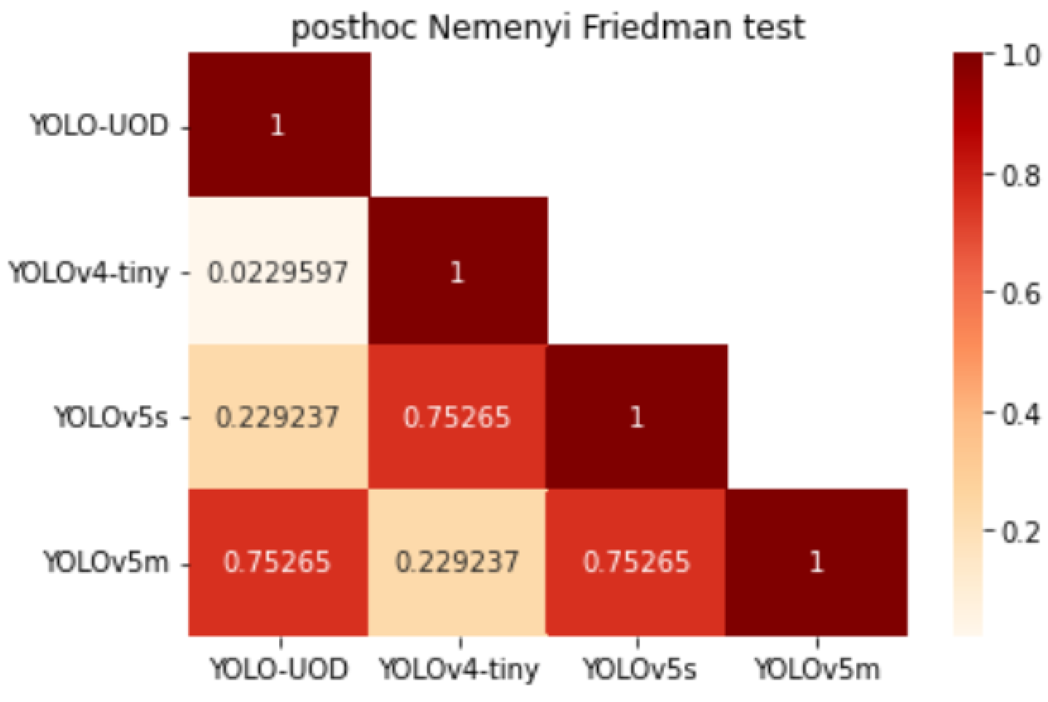
4.2.3. Statistical Analysis

To demonstrate whether there is a significant difference in performance between the proposed YOLO-UOD and YOLOv4-tiny, YOLOv5s, and YOLOv5m, a statistical test between these algorithms is conducted. In this work, the original divided dataset is recorded as $D_1$. The dataset is then randomly divided twice and labeled $D_2$ and $D_3$ per Section 4.1.1’s strategy, and these algorithms are retrained on it. Afterward, the Friedman test and post hoc Nemenyi test [31] are performed on mAP scores of different algorithms on each dataset.

The confusion matrix shown in Figure 9 records the p-value matrix returned by the Friedman test with the post hoc Nemenyi test. The p-value in Figure 9 is a number that describes statistical significance, and the assumption that two algorithms perform the same in accuracy can be rejected when the p-value < 0.05. Figure 9 shows that the p-value between YOLO-UOD and YOLOv4-tiny is 0.0229597 < 0.05, suggesting that the performance of these two algorithms is significantly different. Although the p-value between YOLO-UOD and YOLOv5 does not show a significant difference, the YOLO-UOD has a faster speed in inference. Through the above statistical analysis, it can be proved that the YOLO-UOD has a better balance of speed and accuracy.

5. Conclusions

In view of the disappointing problem of the accuracy and speed of underwater object detection, this paper proposed a YOLO-UOD optimization algorithm based on the research of YOLOv4-tiny.

Experimental results on the Brackish underwater dataset show that the proposed method with the symmetric FPN-Attention module and the symmetric dilated convolutional module can effectively capture valuable features and contextual information and preserve deep features. Its detection mAP score for underwater objects reaches 87.88%, which is higher than YOLOv4-Tiny’s score of 77.38% and better than YOLOv5s and YOLOv5m.

Through significant non-parametric tests on YOLOv4-tiny, YOLOv5s, YOLOv5m, and YOLO-UOD, the results show that the proposed YOLO-UOD is significantly different from YOLOv4-tiny and YOLO-UOD has improved underwater object detection performance. Further analysis shows that although there is no significant difference in performance between YOLO-UOD and YOLOv5m, the inference speed of YOLO-UOD is much faster, suggesting that YOLO-UOD achieves a good balance of speed and accuracy.

However, the proposed YOLO-UOD algorithm still has a certain loss in inference speed (0.63 FPS slower than YOLOv4-tiny), and its applicability to more underwater scenes still needs further research. Therefore, we will continue to study the performance of YOLO-UOD in various underwater scenarios and overcome the disadvantage of inference speed loss.

References

1. Mahmood, A.; Bennamoun, M.; An, S.; Sohel, F.A.; Boussaid, F.; Hovey, R.; Kendrick, G.A.; Fisher, R.B. Deep Image Representations for Coral Image Classification. IEEE J. Ocean. Eng. 2019, 44, 121–131. [Google Scholar] [CrossRef]
2. Kim, B.; Yu, S.C. Imaging sonar based real-time underwater object detection utilizing AdaBoost method. Underw. Technol. IEEE 2017, 1–5. [Google Scholar] [CrossRef]
3. Saini, A.; Biswas, M. Object detection in underwater image by detecting edges using adaptive thresholding. In Proceedings of the 2019 3rd International Conference on Trends in Electronics and Informatics (ICOEI), Tirunelveli, India, 23–25 April 2019; pp. 628–632. [Google Scholar]
4. Wang, C.C.; Samani, H.; Yang, C.Y. Object Detection with Deep Learning for Underwater Environment. In Proceedings of the 2019 4th International Conference on Information Technology Research (ICITR), Moratuwa, Sri Lanka, 10–13 December 2019; pp. 1–6. [Google Scholar]
5. Yang, H.; Liu, P.; Hu, Y.Z.; Fu, J. Research on underwater object recognition based on YOLOv3. Microsyst. Technol. 2021, 27, 1837–1844. [Google Scholar] [CrossRef]
6. Chen, L.Y.; Zheng, M.C.; Dan, S.Q.; Luo, W.; Yao, L. Underwater Target Recognition Based on Improved YOLOv4 Neural Network. Electronics 2021, 10, 1634. [Google Scholar] [CrossRef]
7. Wang, C.Y.; Bochkovskiy, A.; Liao, H.Y.M. Scaled-yolov4: Scaling cross stage partial network. In Proceedings of the IEEE/CVF Conference on Computer Vision and Pattern Recognition, Nashville, TN, USA, 20–25 June 2021; pp. 13029–13038. [Google Scholar]
8. Yu, F.; Koltun, V. Multi-scale context aggregation by dilated convolutions. arXiv 2015, arXiv:1511.07122. [Google Scholar]
9. Pedersen, M.; Bruslund Haurum, J.; Gade, R.; Moeslund, T.B. Detection of marine animals in a new underwater dataset with varying visibility. In Proceedings of the IEEE/CVF Conference on Computer Vision and Pattern Recognition Workshops, Long Beach, CA, USA, 15–20 June 2019; pp. 18–26. [Google Scholar]
10. Chen, C.; Zheng, Z.; Huang, Y.; Ding, X.; Yu, Y. I3net: Implicit instance-invariant network for adapting one-stage object detectors. In Proceedings of the IEEE/CVF Conference on Computer Vision and Pattern Recognition, Nashville, TN, USA, 20–25 June 2021; pp. 12576–12585. [Google Scholar]
11. Wu, P.; Li, H.; Zeng, N.; Li, F. FMD-Yolo: An efficient face mask detection method for COVID-19 prevention and control in public. Image Vis. Comput. 2022, 117, 104341. [Google Scholar] [CrossRef] [PubMed]
12. Jiang, Z.; Liu, Y.; Yang, C.; Liu, J.; Gao, P.; Zhang, Q.; Xiang, S.; Pan, C. Learning where to focus for efficient video object detection. In European Conference on Computer Vision; Springer: Cham, Switzerland, 2020; pp. 18–34. [Google Scholar]
13. Sultani, W.; Chen, C.; Shah, M. Real-world anomaly detection in surveillance videos. In Proceedings of the IEEE Conference on Computer Vision and Pattern Recognition, Salt Lake City, UT, USA, 18–23 June 2018; pp. 6479–6488. [Google Scholar]
14. Girshick, R.; Donahue, J.; Darrell, T.; Malik, J. Rich feature hierarchies for accurate object detection and semantic segmentation. In Proceedings of the IEEE Conference on Computer Vision and Pattern Recognition, Columbus, OH, USA, 23–28 June 2014; pp. 580–587. [Google Scholar]
15. Girshick, R. Fast r-cnn. In Proceedings of the IEEE International Conference on Computer Vision, Santiago, Chile, 7–13 December 2015; pp. 1440–1448. [Google Scholar]
16. Ren, S.; He, K.; Girshick, R.; Sun, J. Faster R-CNN: Towards Real-Time Object Detection with Region Proposal Networks. IEEE Trans. Pattern Anal. Mach. Intell. 2017, 39, 1137–1149. [Google Scholar] [CrossRef] [PubMed]
17. Liu, W.; Anguelov, D.; Erhan, D.; Szegedy, C.; Reed, S.; Fu, C.Y.; Berg, A.C. Ssd: Single shot multibox detector. In European Conference on Computer Vision; Springer: Cham, Switzerland, 2016; pp. 21–37. [Google Scholar]
18. Lin, T.Y.; Goyal, P.; Girshick, R.; He, K.; Dollár, P. Focal loss for dense object detection. In Proceedings of the IEEE International Conference on Computer Vision, Venice, Italy, 22–29 October 2017; pp. 2980–2988. [Google Scholar]
19. Tian, Z.; Shen, C.; Chen, H.; He, T. Fcos: Fully convolutional one-stage object detection. In Proceedings of the IEEE/CVF International Conference on Computer Vision, Seoul, Korea, 27 October–3 November 2019; pp. 9627–9636. [Google Scholar]
20. Redmon, J.; Divvala, S.; Girshick, R.; Farhadi, A. You only look once: Unified, real-time object detection. In Proceedings of the IEEE Conference on Computer Vision and Pattern Recognition, Las Vegas, NV, USA, 27–30 June 2016; pp. 779–788. [Google Scholar]
21. Redmon, J.; Farhadi, A. YOLO9000: Better, faster, stronger. In Proceedings of the IEEE Conference on Computer Vision and Pattern Recognition, Honolulu, HI, USA, 21–26 July 2017; pp. 7263–7271. [Google Scholar]
22. Redmon, J.; Farhadi, A. Yolov3: An incremental improvement. arXiv 2018, arXiv:1804.02767. [Google Scholar]
23. Bochkovskiy, A.; Wang, C.Y.; Liao, H.Y.M. Yolov4: Optimal speed and accuracy of object detection. arXiv 2020, arXiv:2004.10934. [Google Scholar]
24. Wang, C.Y.; Liao, H.Y.M.; Wu, Y.H.; Chen, P.Y.; Hsieh, J.W.; Yeh, I.H. CSPNet: A new backbone that can enhance learning capability of CNN. In Proceedings of the IEEE/CVF Conference on Computer Vision and Pattern Recognition Workshops, Seattle, WA, USA, 14–19 June 2020; pp. 390–391. [Google Scholar]
25. Lin, T.Y.; Dollár, P.; Girshick, R.; He, K.; Hariharan, B.; Belongie, S. Feature pyramid networks for object detection. In Proceedings of the IEEE Conference on Computer Vision and Pattern Recognition, Honolulu, HI, USA, 21–26 July 2017; pp. 2117–2125. [Google Scholar]
26. Hu, J.; Shen, L.; Sun, G. Squeeze-and-excitation networks. In Proceedings of the IEEE Conference on Computer Vision and Pattern Recognition, Salt Lake City, UT, USA, 18–23 June 2018; pp. 7132–7141. [Google Scholar]
27. Woo, S.; Park, J.; Lee, J.Y.; Kweon, I.S. Cbam: Convolutional block attention module. In Proceedings of the European Conference on Computer Vision (ECCV), Munich, Germany, 8–14 September 2018; pp. 3–19. [Google Scholar]
28. Wang, Q.; Wu, B.; Zhu, P.; Li, P.; Zuo, W.; Hu, Q. ECA-Net: Efficient Channel Attention for Deep Convolutional Neural Networks. In Proceedings of the 2020 IEEE/CVF Conference on Computer Vision and Pattern Recognition (CVPR), Seattle, WA, USA, 13–19 June 2020. [Google Scholar]
29. Szegedy, C.; Vanhoucke, V.; Ioffe, S.; Shlens, J.; Wojna, Z. Rethinking the inception architecture for computer vision. In Proceedings of the IEEE Conference on Computer Vision and Pattern Recognition, Las Vegas, NV, USA, 27–30 June 2016; pp. 2818–2826. [Google Scholar]
30. Padilla, R.; Passos, W.L.; Dias, T.L.B.; Netto, S.L.; Da Silva, E.A. A comparative analysis of object detection metrics with a companion open-source toolkit. Electronics 2021, 10, 279. [Google Scholar] [CrossRef]
31. Trawiński, B.; Smętek, M.; Telec, Z.; Lasota, T. Nonparametric statistical analysis for multiple comparison of machine learning regression algorithms. Int. J. Appl. Math. Comput. Sci. 2012, 22, 867–881. [Google Scholar] [CrossRef]
Figure 1. Basic framework of object detection.
Symmetry 14 01669 g001
Figure 2. Architecture of YOLOv4-tiny network.
Symmetry 14 01669 g002
Figure 3. Overall flow chart of YOLO-UOD.
Symmetry 14 01669 g003
Figure 4. Receptive field size of the dilated convolution.
Symmetry 14 01669 g004
Figure 5. Symmetric dilated convolutional module.
Symmetry 14 01669 g005
Figure 6. Symmetric FPN-Attention module structure.
Symmetry 14 01669 g006
Figure 7. Brackish underwater dataset. (a) Big fish. (b) Small fish. (c) Starfish. (d) Shrimp. (e) Crab. (f) Jellyfish.
Symmetry 14 01669 g007
Figure 8. Display of test results.
Symmetry 14 01669 g008
Figure 9. p-values of statistical analysis.
Symmetry 14 01669 g009