A Comparative Study of Three Mathematical Models for the Interaction between the Human Immune System and a Virus

Abstract

In this paper, we will consider three deterministic models for the study of the interaction between the human immune system and a virus: the logistic model, the Gompertz model, and the generalized logistic model (or Richards model). A qualitative analysis of these three models based on dynamical systems theory will be performed by studying the local behavior of the equilibrium points and obtaining the local dynamics properties from the linear stability point of view. Additionally, we will compare these models in order to understand which is more appropriate to model the interaction between the human immune system and a virus. Some natural medical interpretations will be obtained, which are available for all three models and can be useful to the medical community.

1. Introduction

According to the basic immunology treaties around the medical scientific world, from the structural point of view, the human immune system is formed by organs, cells, and molecules [1]. The organs of the human immune system are tonsils and adenoids, the thymus, lymph nodes, spleen, payer’s patches, appendix, lymphatic vessels, and bone marrow. The cells of the immune system are lymphocytes (T-lymphocytes, B-lymphocytes, plasma cells, and natural killer lymphocytes), monocytes, macrophages, and granulocytes (neutrophils, eosinophils, and basophils). The molecules of the immune system are the antibodies, complements, cytokines, interleukines, and interferons [1,2]. Immunity is the resistance of the host body to pathogen agents and their toxic effects. Every human body has a nonspecific response (innate immunity) and a specific response (acquired immunity) [1,2,3]. The innate immunity is based on mechanisms already existing before the pathogen agent infects the host and is the first line of the body’s defense, but it has no memory for subsequent exposure and is based on nonspecific mechanisms. Instead, the adaptive acquired immunity develops after the entrance of a pathogenic agent (virus, microbe, bacteria, parasites, or fungi) into the host and comes into action after innate immunity fails to get rid of these invaders. This acquired immunity has the memory to fight with pathogens in subsequent exposures and uses the specific cells (i.e., T cells (or cell-mediated) and B cells (or antibody-mediated)) [1,2,3].

Recently, a lot of modern epidemiological models, including mathematical models of the COVID-19 epidemic and other models for the spread of diseases such as Ebola, tuberculosis, or influenza, were studied by many experts in the dynamics of infectious diseases in [4,5,6,7].

In this paper, we consider the interaction between the human body’s immune system and a pathogenic invader, and we try to find an appropriate deterministic mathematical model in order to study the fight of the immune system with the invader [8,9]. These kinds of first-order systems of ordinary differential equations represent a class of Kolmogorov systems, and they are used very often in order to obtain mathematical models for the dynamics of populations, prey–predator ecological models, or other models for the spread of diseases or for the growth of tumors [10,11,12,13,14].

We will denote by $x_1\left(t\right)$ the level in time of the immune system (antibody level) and by $v\left(t\right)$ the level of the virus. More exactly, $v\left(t\right)$ represents the number of virus cells which exist in a body at time t. As soon as it notices the presence of a virus in the body, the immune system will fight with the virus (e.g., the present coronavirus, COVID-19) in order to stop its multiplication and eliminate it. Consider the time as being continuous, where $t\ge 0$. Thus, ${\dot{x}}_1\left(t\right)$ and $\dot{v}\left(t\right)$ are the rates of change of these two quantities in a short unit of time, where ${\dot{x}}_1\left(t\right)=\frac{d{x}_1}{dt}$ and $\dot{v}\left(t\right)=\frac{dv}{dt}$. Following the ideas of G. Moza from [15], this model is based on the following three hypotheses:

Hypothesis 1.

In the absence of a virus, the quantity of antibodies $x_1\left(t\right)$ can be present in the human body up to a threshold value $K_1$. This hypothesis is based on the fact that the human body may have an innate immunity and also humoral and cellular immunity after prior possible contact with the virus. Thus, in the first stage, before a present contact with the virus $v\left(t\right)$, we consider that the evolution law of $x_1\left(t\right)$ is the following:

$${\dot{x}}_1=a_1{x}_1-b_1{x}_1^2$$

with $a_1>0$ and $b_1>0$. Taking into account that the solution of the prevoius equation with the initial condition $x_1\left(0\right)=x_{10}$ is

$$x_1\left(t\right)={\displaystyle \frac{K_1}{1+\left(\frac{K_1}{x_{10}}-1\right)e^{-a_{1}t}}}$$

then one can observe that $x_1\left(t\right)\to K_1$ for $t\to \infty$, where $K_1=\frac{a_1}{b_1}$ is the threshold value.

If the term $-b_1{x}_1^2$ is missing, then $x_1\left(t\right)$ increases exponentially when $t\to \infty$, because in this case ($b_1=0$), the general solution of the equation in $x_1$ will be $x_1\left(t\right)=a_1{x}_{10}{e}^{t{a}_1}$. Otherwise, if $b_1>0$, then we find that the maximum threshold value of the antibody level $x_1$ is $\frac{a_1}{b_1}=K_1$.

Hypothesis 2.

Normally, in an healthy body without autoimmune diseases, the antibodies of the immune system do not attack other normal cells of the body. Thus, they can be destroyed only due to viruses, and as such, a term in the form $-c_1{x}_{1}v$ should be added to each equation in $x_1\left(t\right)$, where $v\left(t\right)$ is the number of virus cells which exist in the human body at time t.

Hypothesis 3.

In the absence of the immune system of the body, the virus would multiply indefinitely and exponentially, with $v\left(t\right)$ satisfying the law $\dot{v}=p_{2}v$. However, of course, in the presence of the immune system, the number of virus cells will decrease, and consequently, we must add the terms $-p_1{x}_{1}v$ to the evolution law of $v\left(t\right)$.

If we denote the variable v by $x_2$, then we can conclude that these hypotheses lead us to the following two-dimensional first-order differential system with five parameters, given by

$$\left\{\begin{array}{ccc}\hfill {\dot{x}}_1& =& a_1{x}_1-b_1{x}_1^2-c_1{x}_1{x}_2\hfill \\ \hfill {\dot{x}}_2& =& p_2{x}_2-p_1{x}_1{x}_2\hfill \end{array}\right.$$

(1)

where $a_1>0$, $b_1>0$, $c_1>0$, $p_1>0$, and $p_2>0$.

Obviously, the model has medical relevance when $x_i\ge 0$, $i=1,2$. Therefore, the solutions of the system lie in the set

$${\mathsf{\Sigma }}_{+}^0=\left\{(x_1,x_2)\in {\mathbf{R}}^2\mid x_i\ge 0,i=1,2\right\}.$$

Moreover, the lines $\{x_i=0\}$ are invariant manifolds with respect to the flow of the system (i.e., any orbit starting from a point which belongs to ${\mathsf{\Sigma }}_{+}=\left\{(x_1,x_2)\in {\mathbf{R}}^2\mid x_i>0,i=1,2\right\}$ remains in ${\mathsf{\Sigma }}_{+}$). Therefore, the orbits cannot cross any of these two invariant lines, and then the study of the system where it has medical relevance is well-defined in the sense that an orbit starting from a zone with medical relevance does not enter a zone with medical irrelevance, and vice versa.

This deterministic mathematical model of the interaction between the immune system and a pathogenic invader is based on the logistic differential equation

$$\dot{x}=ax-b{x}^2$$

or in the form

$$\dot{x}=ax\left(1-\frac{x}{K}\right),\mathrm{where}K=\frac{a}{b}$$

Next, using the same hypothesis, we can obtain another two models based on the Gompertz equation

$$\dot{x}=ax\left(lnK-lnx\right)$$

and generalized logistic equation (Richards equation):

$$\dot{x}=ax\left(1-{\left(\frac{x}{K}\right)}^{\nu }\right),\mathrm{where}\nu >0.$$

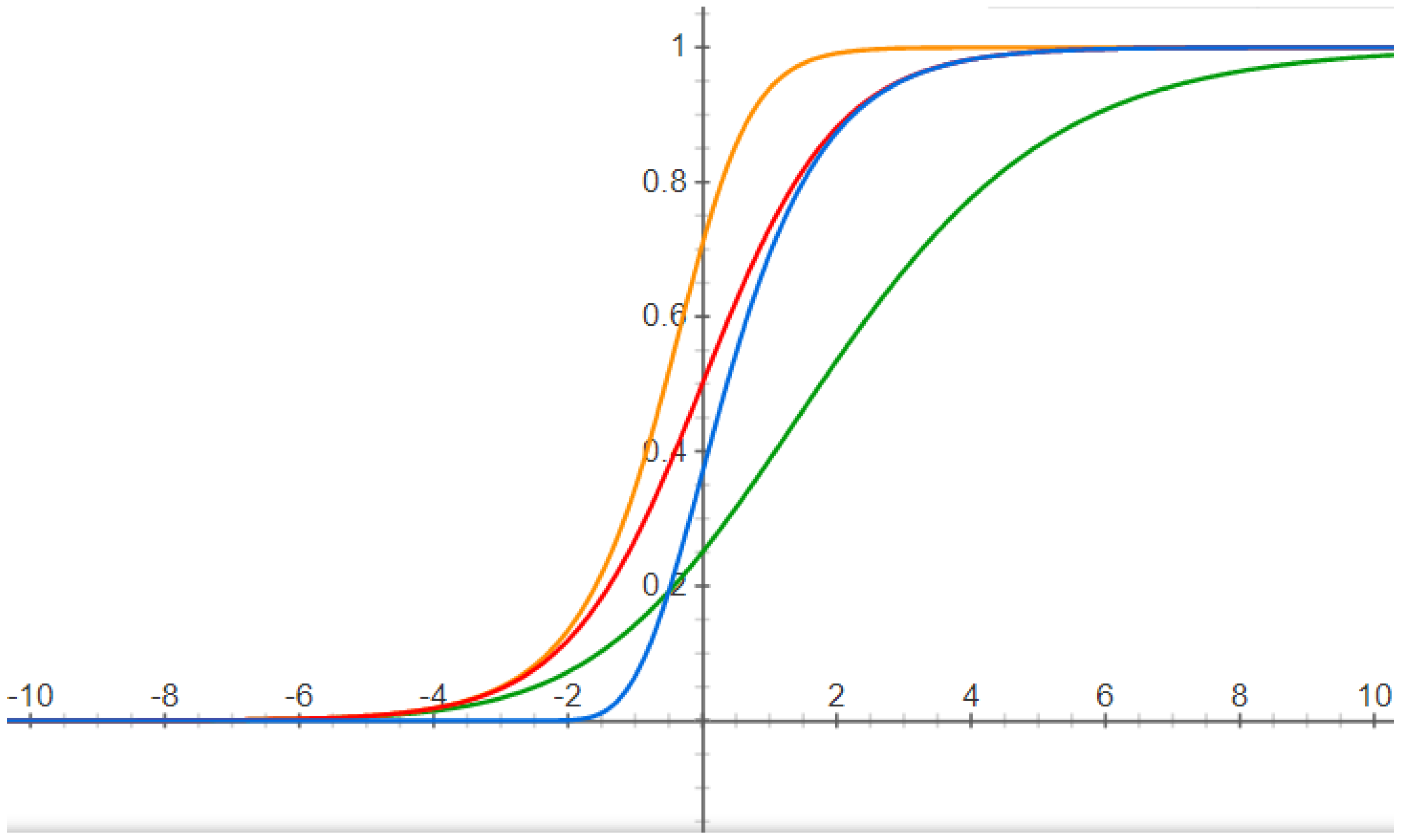
The graphs of the solutions of these ordinary differential equations belong to the so-called S-shaped curves (see Figure 1).

It can be remarked that only the logistic curve is symmetric with respect to the inflection point of $0.5$. The Gompertz curve has a lower inflection point, and the generalized logistic curve can have an inflection point over $0.5$ or up to $0.5$, depending on the parameter $\nu$.

The two-dimensional deterministic model represented by Equation (1) was developed using the logistic model in the second section, following the ideas from the three hypotheses of G. Moza in [15]. For the first time, in the third and the fourth sections, we will use the Gompertz model and the generalized logistic model (or Richards model) in order to construct a deterministic model for the interaction between the human immune system and a virus. Then, these models will be studied from the dynamical systems theory point of view, including the behavior and dynamics properties around the equilibrium points. The generalizations for higher dimensions of these three models will be introduced and studied in Section 5. For all three models, no matter the number of variables, the existence of transcritical bifurcations is obtained, but no Hopf-type bifurcations can occur. Therefore, there are no limit cycles. Finally, a section with relevant conclusions from the epidemiological and medical points of view will be presented.

2. The Logistic Model

The logistic function was introduced by Belgian mathematician Pierre-François Verhulst in a series of three papers [16,17,18] between the years 1838 and 1847. This model was created by Verhulst as a model of population growth by adjusting the exponential growth model through the introduction of a upper threshold called the carrying capacity.

2.1. A Short Presentation

The logistic equation is the following first-order differential equation:

$$\dot{x}=ax-b{x}^2$$

(2)

or equivalently

$$\dot{x}=ax\left(1-\frac{x}{K}\right)$$

(3)

where $K=\frac{a}{b}$ is the carrying capacit and a is the inherent growth rate of the modeled population ($a>0$, $b>0$).

The solution of this differential equation with the initial condition $x_0=x\left(0\right)$ is the logistic function

$$x\left(t\right)=\frac{K}{1+\left(\frac{K}{x_0}-1\right)e^{-at}}$$

(4)

There are two equilibrium points for the dynamical system given by the logistic equation, namely $x_1=0$ and $x_2=K$.

Since $F\left(x\right)=ax\left(1-\frac{x}{K}\right)$ and $\frac{dF}{dx}\left(x\right)=a\left(1-\frac{2x}{K}\right)$, it follows that $\frac{dF}{dx}\left(0\right)=a>0$ and $\frac{dF}{dx}\left(K\right)=-a<0$ (i.e., $x_1=0$ is a repeller, and $x_2=K$ is an attractor).

2.2. The Interaction between the Immune System and a Virus in a Logistic Model

We consider the following system of two differential equations:

$$\left\{\begin{array}{ccc}\hfill {\dot{x}}_1& =& a_1{x}_1-b_1{x}_1^2-c_1{x}_1{x}_2\hfill \\ \hfill {\dot{x}}_2& =& p_2{x}_2-p_1{x}_1{x}_2\hfill \end{array}\right.,$$

(5)

where $x_1>0$ represents the antibody level of the immune system and $x_2=v\ge 0$ represents the concentration of the virus in the body. Here, $K_1=\frac{a_1}{b_1}$ is the carrying capacity of the antibodies, $a_1$ is his inherent growth rate, $p_2$ is the inherent growth rate of the virus, and $c_1$, $p_1$ represent the interaction between the antibodies and virus. All parameters $a_i$, $b_i$, $c_i$, and $p_i$ are strictly positive.

The Jacobi matrix at an equilibrium point $(x_1,x_2)$ is

$$A=\left(\begin{array}{cc}{a}_1-2b_1{x}_1-c_1{x}_2& -c_1{x}_1\\ -p_1{x}_2& p_2-p_1{x}_1\end{array}\right)$$

In order to find the equilibria, by analyzing the system

$$\left\{\begin{array}{c}{x}_1(a_1-b_1{x}_1-c_1{x}_2)=0\hfill \\ x_2(p_2-p_1{x}_1)=0\hfill \end{array}\right.$$

we obtain the following three equlibria: $E_0(0,0)$ with eigenvalues ${\lambda }_1=a_1$ and ${\lambda }_2=p_2$, $E_1\left(\frac{a_1}{b_1},0\right)$ with eigenvalues ${\lambda }_1=-a_1$ and ${\lambda }_2=p_2-p_1\frac{a_1}{b_1}$, and $E_2\left(\frac{p_2}{p_1},\frac{1}{c_1}\left(a_1-b_1\frac{p_2}{p_1}\right)\right)$ with eigenvalues

$${\lambda }_{1,2}=\frac{1}{2p_1}\left(-b_1{p}_2\pm \sqrt{b_1^2{p}_2^2+4p_2{p}_1^2\left(a_1-b_1\frac{p_2}{p_1}\right)}\right).$$

Therefore, we have the following results:

Theorem 1. (a) 

The trivial equilibria $E_0(0,0)$ is always a repeller.

(b) 

The equilibria $E_1$ is an attractor if and only if $\frac{p_2}{p_1}<K_1=\frac{a_1}{b_1}$.

Otherwise, $E_1$ is a saddle point.

(c) 

The equilibria $E_2$ is a saddle point whenever it lies on ${\mathsf{\Sigma }}_{+}$.

Moreover, $E_2\in {\mathsf{\Sigma }}_{+}$ if and only if $\frac{p_2}{p_1}<K_1$ (i.e., $E_1$ is an attractor).

(d) 

The system does not undergo a Hopf bifurcation at $E_2$ on ${\mathsf{\Sigma }}_{+}$.

(e) 

$E_2$ collides with $E_1$ on the line $S:$ $p_2=p_1{K}_1$.

(f) 

The equilibria $E_2$ bifurcates from the equilibria $E_1$ along the line

$S=\left\{(p_1,p_2)\right|p_2=p_1{K}_1\}$ by a transcritical bifurcation.

3. The Gompertz Model

Taking into account that when using the logistic equation, there are a lot of mathematical models for describing the behavior in time of the epidemiological or ecological systems, we will further introduce a new mathematical model for studying the interactions between different kinds of species using the Gompertz model. This model was introduced by British mathematician Benjamin Gompertz in 1825 in order to obtain a law of mortality as well as a demographic model (see [19]). One hundred forty years later in 1964, A.K. Laird used the Gompertz curve to fit data on the growth of tumors [20].

3.1. A Short Presentation

The Gompertz equation is the following first-order differential equation:

$$\dot{x}=axln\frac{K}{x}$$

(6)

or equivalently

$$\dot{x}=ax\left(lnK-lnx\right)$$

(7)

where $K=\frac{a}{b}$ is the carrying capacity and a is the inherent growth rate of the modeled population ($a>0$, $K>0$).

The solution of this differential equation with the initial condition $x_0=x\left(0\right)$ is the Gompertz function

$$x\left(t\right)=K{e}^{-ln\left(\frac{K}{x_0}\right)e^{-at}}$$

(8)

There is a single equilibrium point for the dynamical system given by the Gompertz equation, namely $x_1=K$.

Since $F\left(x\right)=ax\left(lnK-lnx\right)$ and $\frac{dF}{dx}\left(x\right)=aln\frac{K}{x}-a$, it follows that $\frac{dF}{dx}\left(K\right)=-a<0$ (i.e., $x_1=K$ is an attractor).

3.2. The Interaction between the Immune System and a Virus in the Gompertz Model

We consider the following system of two differential equations:

$$\left\{\begin{array}{ccc}\hfill {\dot{x}}_1& =& a_1{x}_{1}ln\frac{K_1}{x_1}-c_1{x}_1{x}_2\hfill \\ \hfill {\dot{x}}_2& =& p_2{x}_2-p_1{x}_1{x}_2\hfill \end{array}\right.$$

(9)

where $x_1>0$ represents the antibody level of the immune system and $x_2=v\ge 0$ is the concentration of the virus in the body. Here, $K_1=\frac{a_1}{b_1}$ is the carrying capacity of the antibodies, $a_1$ is the inherent growth rate, $p_2$ is the inherent growth rate of the virus, and $c_1$ and $p_1$ are the interaction’s coefficients between the antibodies and virus, respectively. All parameters $a_i$, $b_i$, $c_i$, and $p_i$ are strictly positive.

The Jacobi matrix at an equilibrium point $(x_1,x_2)$ is

$$A=\left(\begin{array}{cc}{a}_{1}ln\frac{K_1}{x_1}-a_1-c_1{x}_2& -c_1{x}_1\\ -p_1{x}_2& p_2-p_1{x}_1\end{array}\right)$$

In order to find the equilibrium points, we analyze the system

$$\left\{\begin{array}{c}{x}_1(a_{1}ln\frac{K_1}{x_1}-c_1{x}_2)=0\hfill \\ x_2(p_2-p_1{x}_1)=0\hfill \end{array}\right.$$

We obtain two equlibria: $E_1(K_1,0)$ with eigenvalues ${\lambda }_1=-a_1$ and ${\lambda }_2=p_2-p_1{K}_1$ and $E_2\left(\frac{p_2}{p_1},\frac{a_1}{c_1}ln\left(K_1\frac{p_1}{p_2}\right)\right)$, which exists if and only if $K_1\frac{p_1}{p_2}>1$ (i.e., $\frac{p_2}{p_1}<K_1$).

Otherwise, if $\frac{p_2}{p_1}\ge K_1$, the equilibrium $E_2$ does not exist (i.e., it does not belong to ${\mathsf{\Sigma }}_{+}$).

For $E_2$, we obtain the eigenvalues ${\lambda }_{1,2}=-\frac{1}{2}{a}_1\pm \frac{1}{2}\sqrt{\left(a_1^2+4p_2{a}_{1}ln{K}_1\frac{p_1}{p_2}\right)}$.

Since ${\lambda }_1+{\lambda }_2=-a_1<0$ and ${\lambda }_1{\lambda }_2=-p_2{a}_{1}ln\left(K_1\frac{p_1}{p_2}\right)<0$, it is found that $E_2$ is a saddle point.

In conclusion, we have the following results:

Theorem 2. (a) 

The equilibrium $E_1$ is an attractor if and only if $\frac{p_2}{p_1}<K_1$. Otherwise, $E_1$ is a saddle point.

(b) 

The equilibrium $E_2$ is a saddle point whenever it lies on ${\mathsf{\Sigma }}_{+}$. Moreover, $E_2\in {\mathsf{\Sigma }}_{+}$ if and only if $\frac{p_2}{p_1}<K_1$ (i.e., $E_1$ is an attractor).

(c) 

The system does not undergo a Hopf bifurcation at $E_2$ on ${\mathsf{\Sigma }}_{+}$.

(d) 

$E_2$ collides with $E_1$ on the line $S:$ $p_2=p_1{K}_1$.

(e) 

The equilibrium $E_2$ bifurcates from the equilibrium $E_1$ along the line

$S=\left\{(p_1,p_2)\right|p_2=p_1{K}_1\}$ by a transcritical bifurcation.

4. The Generalized Logistic Model

The generalized logistic function known as Richards’s function is a generalization of the logistic function, with more flexible S-shaped graph curves and an inflection point which depends on a parameter. This function is the solution of the Richards differential equation (RDE), otherwise known as the generalized logistic differential equation, and was used for modeling many growth phenomena from oncology and epidemiology. F. J. Richards proposed this growth function for the first time in 1959 in [21].

4.1. A Short Presentation

The generalized logistic equation (or Richards’s differential equation (RDE)) is the following first-order differential equation:

$$\dot{x}=ax\left(1-{\left(\frac{x}{K}\right)}^{\nu }\right)$$

(10)

where $K=\frac{a}{b}$ is the carrying capacity, a is the inherent growth rate of the modeled population, and $\nu >0$ ($a>0$, $b>0$).

The solution of this differential equation with the initial condition $x_0=x\left(0\right)$ is the generalized logistic function or Richards function:

$$x\left(t\right)=\frac{K}{{\left[1+\left({\left(\frac{K}{x_0}\right)}^{\nu }-1\right)e^{-a\nu t}\right]}^{\frac{1}{\nu }}}$$

(11)

There are two equilibrium points for the dynamical system given by the generalized logistic equation, namely $x_1=0$ and $x_2=K$.

Since $F\left(x\right)=ax\left(1-{\left(\frac{x}{K}\right)}^{\nu }\right)$ and $\frac{dF}{dx}\left(x\right)=a\left(1-2{\left(\frac{x}{K}\right)}^{\nu }\right)$, it follows that $\frac{dF}{dx}\left(0\right)=a>0$ and $\frac{dF}{dx}\left(K\right)=-a<0$ (i.e., $x_1=0$ is a repeller, and $x_2=K$ is an attractor).

Let us remark that for $\nu =1$, the classical logistic equation (Equation (3)) is just a particular case of the Richards differential equation (Equation (10)). Moreover, the Gompertz equation (Equation (7)) can be obtained from the generalized logistic equation (Equation (10)) when $\nu \searrow 0$, provided that $a=O\left(\frac{1}{\nu }\right)$. In fact, for $\nu >0$, being small enough, we can take $a=\frac{r}{\nu }$, with $r>0$, and then the Richards equation $\dot{x}=ax\left(1-{\left(\frac{x}{K}\right)}^{\nu }\right)$ becomes

$$\dot{x}=\frac{r}{\nu }x\left(1-{\left(\frac{x}{K}\right)}^{\nu }\right)=rx\left(\frac{1-e^{\nu ln\left(\frac{x}{K}\right)}}{\nu }\right)=rxln\left(\frac{K}{x}\right)$$

if we take into account that $\frac{1-e^{\nu Y}}{\nu }=\frac{-\nu Y}{\nu }=-Y$ for $\nu >0$ at a very small value. Here, the terms of order greater than two from $e^{\nu Y}={\displaystyle \sum _{n=0}^{+\infty }}\frac{{\left(\nu Y\right)}^n}{n!}$ are neglected because v is very small.

4.2. The Interaction between the Immune System and a Virus through the Generalized Logistic Model

We consider the following system of two differential equations:

$$\left\{\begin{array}{ccc}\hfill {\dot{x}}_1& =& a_1{x}_1\left(1-{\left(\frac{x_1}{K_1}\right)}^{\nu }\right)-c_1{x}_1{x}_2\hfill \\ \hfill {\dot{x}}_2& =& p_2{x}_2-p_1{x}_1{x}_2\hfill \end{array}\right.,$$

(12)

where $x_1>0$ represents the antibody level of the immune system and $x_2=v\ge 0$ is the concentration of the virus in the body. Here, $K_1=\frac{a_1}{b_1}$ is the carrying capacity of the antibodies, $a_1$ is their inherent growth rate, $p_2$ is the inherent growth rate of the virus, and $c_1$ and $p_1$ are the interaction’s coefficients between the antibodies and the virus, respectively. All parameters $a_i$, $b_i$, $c_i$, $p_i$, and $\nu \in (0,1)$ are strictly positive.

The Jacobi matrix at an equilibrium point $(x_1,x_2)$ is

$$A=\left(\begin{array}{cc}{a}_1-a_1(1+\nu ){\left(\frac{x_1}{K_1}\right)}^{\nu }-c_1{x}_2& -c_1{x}_1\\ -p_1{x}_2& p_2-p_1{x}_1\end{array}\right).$$

In order to find the equilibrium points, by analyzing the system

$$\left\{\begin{array}{c}{x}_1\left(a_1\left(1-{\left(\frac{x_1}{K_1}\right)}^{\nu }\right)-c_1{x}_2\right)=0\hfill \\ x_2(p_2-p_1{x}_1)=0\hfill \end{array}\right.$$

we obtain the following three equilibria: $E_0(0,0)$ with eigenvalues ${\lambda }_1=a_1$ and ${\lambda }_2=p_2$, $E_1\left(K_1,0\right)$ with eigenvalues ${\lambda }_1=-a_1\nu$ and ${\lambda }_2=p_2-p_1{K}_1$, and $E_2\left(\frac{p_2}{p_1},\frac{a_1}{c_1}\left(1-{\left(\frac{p_2}{p_1{K}_1}\right)}^{\nu }\right)\right)$ with eigenvalues ${\lambda }_{1,2}=-\frac{1}{2}{a}_1\nu {\left(\frac{p_2}{p_1{K}_1}\right)}^{\nu }\pm \frac{1}{2}\sqrt{a_1^2{\nu }^2{\left(\frac{p_2}{p_1{K}_1}\right)}^{2\nu }+4p_2{a}_1-4p_2{a}_1{\left(\frac{p_2}{p_1{K}_1}\right)}^{\nu }}$.

For $E_2$, since ${\lambda }_1+{\lambda }_2=-a_1\nu e^{\nu ln\frac{p_2}{p_1{K}_1}}<0$ and ${\lambda }_1{\lambda }_2=-p_2{a}_1\left(1-{\left(\frac{p_2}{p_1{K}_1}\right)}^{\nu }\right)<0$, it follow that $E_2$ is a saddle point whenever it belongs to ${\mathsf{\Sigma }}_{+}$.

Then, we have the following results:

Theorem 3. (a) 

The trivial equilibrium $E_0(0,0)$ is always a repeller.

(b) 

The equilibrium $E_1$ is an attractor if and only if $\frac{p_2}{p_1}<K_1$. Otherwise, $E_1$ is a saddle point.

(c) 

The equilibrium $E_2$ is a saddle point whenever it lies on ${\mathsf{\Sigma }}_{+}$. Moreover, $E_2\in {\mathsf{\Sigma }}_{+}$ if and only if $\frac{p_2}{p_1}<K_1$ (i.e., $E_1$ is an attractor).

(d) 

The system does not undergo a Hopf bifurcation at $E_2$ on ${\mathsf{\Sigma }}_{+}$.

(e) 

$E_2$ collides with $E_1$ on the line $S:$ $p_2=p_1{K}_1$.

(f) 

The equilibrium $E_2$ bifurcates from the equilibrium $E_1$ along the line

$S=\left\{(p_1,p_2)\right|p_2=p_1{K}_1\}$ by a transcritical bifurcation.

5. Generalizations for $\mathit{n}\ge \mathbf{3}$

If we consider a mathematical model with interaction between two, three, or more types of human body immunities (or antibodies) and a virus, then we can similarly consider a system with three, four, or more differential equations using the logistic model, Gompertz model, or generalized logistic model.

For the three-dimensional model built by the logistic model, complete results can be found in the paper by G. Moza [15]. For the extended four-dimensional model, the results can be found in [22]. For a three-dimensional system, there are at most seven equilibrium points, among which only one can be an attractor. The rest of the equilibria are saddle points (if they exist), with the exception of the trivial equilibrium (the origin O), which is a repeller. More precisely, the equilibrium $(K_1,K_2,0)$ is an attractor if $p_3<p_1{K}_1+p_2{K}_2$, where $K_1$ and $K_2$ are the threshold values of the antibodies [15]. Similar results were obtained in [22] for the four-dimensional model, but the number of discovered equilibrium points was larger, having up to 15 equilibria. A generalization for higher dimensions can be discussed, but the number of equilibria becomes huge. For example, for a six-dimensional model, it will obtain up to 63 points of equilibrium [22].

However, if we consider the Gompertz model with two, three, or more types of human body immunities (or antibodies) and a virus, then the number of equilibria remains constant, and the obtained results do not depend of the number of variables of the system from the qualitative point of view.

For $n=3$, we consider the following system of three differential equations:

$$\left\{\begin{array}{ccc}\hfill {\dot{x}}_1& =& a_1{x}_{1}ln\frac{K_1}{x_1}-c_1{x}_1{x}_3\hfill \\ \hfill {\dot{x}}_2& =& a_2{x}_{2}ln\frac{K_2}{x_2}-c_2{x}_2{x}_3\hfill \\ \hfill {\dot{x}}_3& =& p_3{x}_3-p_1{x}_1{x}_3-p_2{x}_2{x}_3\hfill \end{array}\right.,$$

(13)

where $x_1$, $x_2>0$ and $x_3=v\ge 0$.

The Jacobi matrix at an equilibrium point $(x_1,x_2,x_3)$ is

$$A=\left(\begin{array}{ccc}{a}_{1}ln\frac{K_1}{x_1}-a_1-c_1{x}_3& 0& -c_1{x}_1\\ 0& a_{2}ln\frac{K_2}{x_2}-a_2-c_2{x}_3& -c_2{x}_2\\ -p_1{x}_3& -p_2{x}_3& p_3-p_1{x}_1-p_2{x}_2\end{array}\right)$$

In order to find the equilibrium points, by analyzing the system

$$\left\{\begin{array}{c}\hfill x_1(a_{1}ln\frac{K_1}{x_1}-c_1{x}_3)=0\\ \hfill x_2(a_{2}ln\frac{K_2}{x_2}-c_2{x}_3)=0\\ \hfill x_3(p_3-p_1{x}_1-p_2{x}_2)=0\end{array}\right.$$

we obtain the following two equilibria: $E_1(K_1,K_2,0)$ with eigenvalues ${\lambda }_1=-a_1$, ${\lambda }_2=-a_2$ and ${\lambda }_3=p_3-p_1{K}_1-p_2{K}_2$ and $E_2(x_1^{*},x_2^{*},x_3^{*})$, which exists if $p_3-p_1{K}_1-p_2{K}_2<0$ (i.e., $E_1$ is an attractor), where $x_1^{*}$, $x_2^{*}$, $x_3^{*}$ are strictly positive real numbers which satisfy $\frac{a_i}{c_i}ln\frac{K_i}{x_i^{*}}=x_3^{*}$ or $x_i^{*}=K_i{e}^{-x_3^{*}\frac{c_i}{a_i}}$ ($i=1,2$) and $p_1{x}_1^{*}+p_2{x}_2^{*}=p_3$.

The characteristic polynomial at $E_2$ is

$$P\left(\lambda \right)={\lambda }^3+\left(a_1+a_2\right){\lambda }^2+\left(a_1{a}_2-x_3^{*}\left(c_2{x}_2^{*}{p}_2+p_1{c}_1{x}_1^{*}\right)\right)\lambda -x_3^{*}\left(a_1{c}_2{x}_2^{*}{p}_2+p_1{c}_1{x}_1^{*}{a}_2\right).$$

Taking into account that ${\alpha }_2=a_1+a_2>0$, ${\alpha }_1=\left(a_1{a}_2-x_3^{*}\left(c_2{x}_2^{*}{p}_2+p_1{c}_1{x}_1^{*}\right)\right)$, ${\alpha }_0=-x_3^{*}\left(a_1{c}_2{x}_2^{*}{p}_2+v{p}_1{c}_1{x}_1^{*}{a}_2\right)<0$, and ${\alpha }_2{\alpha }_1-{\alpha }_0=a_1{a}_2(a_1+a_2)-x_3^{*}\left(p_1{c}_1{x}_1^{*}{a}_1+c_2{x}_2^{*}{p}_2{a}_2\right)$, following the Hurwitz criterion, the result is that $E_2$ is not an attractor.

Moreover, because we have ${\lambda }_1+{\lambda }_2+{\lambda }_3=-(a_1+a_2)<0$, ${\lambda }_1{\lambda }_2+{\lambda }_2{\lambda }_3+{\lambda }_3{\lambda }_1=\left(a_1{a}_2-x_3^{*}\left(c_2{x}_2^{*}{p}_2+p_1{c}_1{x}_1^{*}\right)\right)$, ${\lambda }_1{\lambda }_2{\lambda }_3=x_3^{*}\left(a_1{c}_2{x}_2^{*}{p}_2+p_1{c}_1{x}_1^{*}{a}_2\right)>0$, and ${\lambda }_1^2+{\lambda }_2^2+{\lambda }_3^2={(a_1+a_2)}^2-2\left(a_1{a}_2-x_3^{*}\left(c_2{x}_2^{*}{p}_2+p_1{c}_1{x}_1^{*}\right)\right)=a_1^2+a_2^2+2c_2{x}_2^{*}{p}_2{x}_3^{*}+2p_1{x}_3^{*}{c}_1{x}_1^{*}>0$, it follows that $E_2$ is a saddle point whenever it exists.

Next, we obtain the following results:

Theorem 4. (a) 

The equilibrium $E_1(K_1,K_2,0)$ is an attractor if and only if

$p_3-p_1{K}_1-p_2{K}_2<0$. Otherwise, $E_1(K_1,K_2,0)$ is a saddle point.

(b) 

The equilibrium $E_2$ is a saddle point whenever it lies on ${\mathsf{\Sigma }}_{+}$. Moreover, $E_2\in {\mathsf{\Sigma }}_{+}$ if and only if $p_3-p_1{K}_1-p_2{K}_2<0$ (i.e., $E_1$ is an attractor).

(c) 

The system does not undergo a fold-Hopf bifurcation at $E_2$.

(d) 

$E_2$ collides with $E_1$ on the surface $S:$ $p_1{x}_1+p_2{x}_2=p_3$.

(e) 

The equilibrium $E_2$ bifurcates from $E_1$ along the surface

$$S=\left\{(p_1,p_2,p_3)\right|p_3=p_1{K}_1+p_2{K}_2\}$$

by a transcritical bifurcation.

For $n=4$, we consider the following system of four differential equations:

$$\left\{\begin{array}{ccc}\hfill {\dot{x}}_1& =& a_1{x}_{1}ln\frac{K_1}{x_1}-c_1{x}_1{x}_4\hfill \\ \hfill {\dot{x}}_2& =& a_2{x}_{2}ln\frac{K_2}{x_2}-c_2{x}_2{x}_4\hfill \\ \hfill {\dot{x}}_3& =& a_3{x}_{3}ln\frac{K_3}{x_3}-c_3{x}_3{x}_4\hfill \\ \hfill {\dot{x}}_4& =& p_4{x}_4-p_1{x}_1{x}_4-p_2{x}_2{x}_4-p_3{x}_3{x}_4\hfill \end{array}\right.,$$

(14)

where $x_1$, $x_2$, $x_3>0$ and $x_4=v\ge 0$.

The Jacobi matrix at an equilibrium point $(x_1,x_2,x_3,x_4)$ is

$$\left(\begin{array}{cccc}{a}_{1}ln\frac{K_1}{x_1}-a_1-c_1{x}_4& 0& 0& -c_1{x}_1\\ 0& a_{2}ln\frac{K_2}{x_2}-a_2-c_2{x}_4& 0& -c_2{x}_2\\ 0& 0& a_{3}ln\frac{K_3}{x_3}-a_3-c_3{x}_4& -c_3{x}_3\\ -p_1{x}_4& -p_2{x}_4& -p_3{x}_4& p_4-p_1{x}_1-p_2{x}_2-p_3{x}_3\end{array}\right)$$

In order to find the equilibrium points, by analyzing the system

$$\left\{\begin{array}{c}\hfill x_1(a_{1}ln\frac{K_1}{x_1}-c_1{x}_4)=0\\ \hfill x_2(a_{2}ln\frac{K_2}{x_2}-c_2{x}_4)=0\\ \hfill x_3(a_{3}ln\frac{K_3}{x_3}-c_3{x}_4)=0\\ \hfill x_4\left(p_4-p_1{x}_1-p_2{x}_2-p_3{x}_3\right)=0\end{array}\right.$$

we obtain the following two equilibria: $E_1(K_1,K_2,K_3,0)$ with eigenvalues ${\lambda }_1=-a_1$, ${\lambda }_2=-a_2$, ${\lambda }_3=-a_3$, and ${\lambda }_4=p_4-p_1{K}_1-p_2{K}_2-p_3{K}_3$ and $E_2(x_1^{*},x_2^{*},x_3^{*},x_4^{*})$, which exists if and only if $p_4-p_1{K}_1-p_2{K}_2-p_3{K}_3<0$ (i.e., $E_1$ is an attractor), where $x_1^{*}$, $x_2^{*}$, $x_3^{*}$, and $x_4^{*}$ are strictly positive real numbers which satisfy $\frac{a_i}{c_i}ln\frac{K_i}{x_i^{*}}=x_4^{*}$ or $x_i^{*}=K_i{e}^{-x_4^{*}\frac{c_i}{a_i}}$ ($i=1,2,3$) and $p_1{x}_1^{*}+p_2{x}_2^{*}+p_3{x}_3^{*}=p_4$.

The characteristic polynomial at $E_2$ is $P\left(\lambda \right)={\lambda }^4+{\alpha }_3{\lambda }^3+{\alpha }_2{\lambda }^2+{\alpha }_1\lambda +{\alpha }_0$, where ${\alpha }_3=a_1+a_2+a_3$, ${\alpha }_2=a_1{a}_2+a_2{a}_3+a_3{a}_1-x_4^{*}\left(x_1^{*}{c}_1{p}_1+x_2^{*}{c}_2{p}_2+x_3^{*}{c}_3{p}_3\right)$, ${\alpha }_1=a_1{a}_2{a}_3-x_4^{*}\left[x_1^{*}{c}_1{p}_1\left(a_2+a_3\right)+x_2^{*}{c}_2{p}_2\left(a_1+a_3\right)+x_3^{*}{c}_3{p}_3\left(a_1+a_2\right)\right]$, and ${\alpha }_0=-x_4^{*}\left(x_1^{*}{c}_1{p}_1{a}_2{a}_3+x_2^{*}{c}_2{p}_2{a}_1{a}_3+x_3^{*}{c}_3{p}_3{a}_1{a}_2\right)=detA$.

Following the relations of Viète for $P\left(\lambda \right)$, we have ${\lambda }_1{\lambda }_2{\lambda }_3{\lambda }_4={\alpha }_0<0$ and ${\lambda }_1+{\lambda }_2+{\lambda }_3+{\lambda }_4=-{\alpha }_3<0$. Then, it follows that $E_2$ is a saddle point whenever it exists.

Moreover, the characteristic polynomial at $E_2$ has at least two real eigenvalues with different signs. Therefore, we have the following results:

Theorem 5. (a) 

The equilibrium $E_1(K_1,K_2,K_3,0)$ is an attractor if and only if $p_4-p_1{K}_1-p_2{K}_2-p_3{K}_3<0$. Otherwise, $E_1(K_1,K_2,K_3,0)$ is a saddle point.

(b) 

The equilibrium $E_2$ is a saddle point whenever it lies on ${\mathsf{\Sigma }}_{+}$. Moreover, $E_2\in {\mathsf{\Sigma }}_{+}$ if and only if $p_4-p_1{K}_1-p_2{K}_2-p_3{K}_3<0$ (i.e., $E_1$ is an attractor).

(c) 

The system does not undergo a Hopf-Hopf bifurcation at $E_2$.

(d) 

$E_2$ collides with $E_1$ on the hypersurface $S:$ $p_4=p_1{x}_1+p_2{x}_2+p_3{x}_3$.

(e) 

The equilibrium $E_2$ bifurcates from $E_1$ along the hypersurface

$$S=\left\{(p_1,p_2,p_3,p_4)\right|p_4=p_1{x}_1+p_2{x}_2+p_3{x}_3\}$$

by a transcritical bifurcation.

Finally, of course, we can write generalized results available for any $n\ge 3$:

Theorem 6. (a) 

$E_1(K_1,\cdots ,K_{n-1},0)$ is an attractor if and only if $p_n<{\displaystyle \sum _{i=1}^{n-1}}{p}_i{K}_i$. Otherwise, $E_1$ is a saddle point.

(b) 

The equilibrium $E_2$ is a saddle point whenever it lies on ${\mathsf{\Sigma }}_{+}$ (i.e., $E_1$ is an attractor).

Let us remark that the coordinates of the second equilibrium $E_2(x_1^{*},\cdots ,x_{n-1}^{*},x_n^{*})$ are strictly positive real numbers $x_i$ which satisfy $x_i^{*}=K_i{e}^{-x_n^{*}\frac{c_i}{a_i}}$ ($i=\overline{1,n-1}$) and $p_1{x}_1^{*}+\cdots +p_{n-1}{x}_{n-1}^{*}=p_n$. Moreover, $x_i^{*}<K_i$ for all $i=\overline{1,n-1}$.

Obviously, if we want to use the generalized logistic model (Richards model) for the interaction between two, three, or more types of human body immunities (or antibodies) and a virus, then the results will be similar, but the computations are very complicated. This study can be conducted in a future work.

6. Conclusions

Taking into account that our body has at least three types of immunity (innate immunity, humoral immunity and cellular immunity), and these three types of immunity fight jointly with the pathogenic invader (viruses, bacteria, parasites, or fungi) in order to stop its multiplication and eliminate it, in this work, I presented a study about the interactions between the antibodies, cells, and organs of the immune system, as well as other complex human body mechanisms (such as the complement system of the body), and a pathogenic agent, such as COVID-2019. A mathematical approach based on a first-order system of differential equations was used for modeling the interactions, as well as tools from dynamical systems theory for analysis of the models, following the ideas from [15,22]. This study reveals the importance of antibodies in the fight against viruses. Several conclusions relevant to the medical world arise from our study, which are as follows:

1. If the immune system is sufficiently weak when the virus starts to proliferate (e.g., in the neighborhood of the trivial equilibria and the origin O)—that is, the level of antibodies is very small, but the virus concentration is also very small—then the virus has a strong chance to win. This occurs in the neighborhood of the origin O, because O is a repeller (for the logistic and generalized logistic models), and then any orbit $\gamma \left(t\right)$ starting at a point ${\mathbf{x}}_0\in {\mathsf{\Sigma }}_{+}$ close to O will depart from O for a large t value, meaning that $v\left(t\right)$ may progress to infinity when t is large. Therefore, a serious deficiency in the level of immunity in the early stages of virus proliferation may lead to the virus’s victory.

2. If the immunity system is within its normal level (at the carrying capacity) from the first moment it discovers the virus, and if the immune system is in a healthy condition to kill the virus at a high rate ($K_1>\frac{p_2}{p_1}$), then the immune system has the best chance to win the battle with the virus. See the case of the first equilibrium point $E_1(K_1,0)$ when it is an attractor. Indeed, any orbit $\gamma \left(t\right)$ starting at a point ${\mathbf{x}}_0\in {\mathsf{\Sigma }}_{+}$ close to $E_1(K_1,0)$ will converge to $E_1$ for large t values; that is, $v\left(t\right)$ trends toward zero for large t values.

3. If the levels of immunity becomes considerably smaller than their normal concentrations ($x_1<K_1$) at a moment during the battle with the virus, then the virus may win even though the immune system kills the virus at a rate higher than the rate of virus proliferation ($K_1>\frac{p_2}{p_1}$). This is the case of the second equilibrium point $E_2(x_1,v)$, $x_1=\frac{p_2}{p1}$, $v>0$, which is a saddle point whenever it exists. More precisely, any orbit $\gamma \left(t\right)$ starting at a point ${\mathbf{x}}_0\in {\mathsf{\Sigma }}_{+}$ close to $E_2$, ${\mathbf{x}}_0\notin W_{E_2}^s$ will depart from $E_2$ for a large t value, which means $v\left(t\right)$ may progress to infinity when t is large. A stable limit cycle around $E_2$ cannot arise through a Hopf bifurcation since all eigenvalues are real.

4. If the immunity system is within its normal level (at the carrying capacity) from the first moment when it discovers the virus, but the immune system is not able to eliminate the virus at a high rate ($K_1<\frac{p_2}{p_1}$), then the immune system can lose the battle with the virus. This is exactly the situation when the first equilibrium point $E_1$ is a saddle point, and then any orbit $\gamma \left(t\right)$ starting at a point ${\mathbf{x}}_0\in {\mathsf{\Sigma }}_{+}$ close to $E_1$, ${\mathbf{x}}_0\notin W_{E_1}^s$ will depart from $E_1$ for large t values, that means $v\left(t\right)$ may progress to infinity when t is large. A stable limit cycle around $E_1$ cannot arise through a Hopf bifurcation since all eigenvalues are real.

5. If the first equilibrium point $E_1(K_1,0)$ (for which the level of the immunity is at its maximum at the thresholds $K_1$, but the virus concentration is very, very low) is an attractor, then we can conclude that the immune system eliminates the virus for any orbit starting from a point belonging to a small enough neighborhood of $E_1$. However, the virus has another opportunity in the neighborhood of the second equilibrium point $E_2$, which is a saddle point whenever it exists. What is more, this second equilibrium exists if and only if the first equilibrium is an attractor.

Although only the logistic model of the three models has symmetry with respect to the inflection point, these conclusions are available no matter what model is used: logistic, Gompertz, or the generalized logistic model (Richards model). For all models, regardless of the dimensions, the existence of transcritical bifurcations is obtained, but no Hopf-type bifurcations can occur. Therefore, there are no limit cycles.

The results we obtained in this work are natural and tell the medical community to work harder on methods for strengthening the immune system to win battles with pathogenic viruses.