Abstract
This is a review addressing soliton-like states in systems with nonlocal nonlinearity. The work on this topic has long history in optics and related areas. Some results produced by the work (such as solitons supported by thermal nonlinearity in optical glasses, and orientational nonlinearity, which affects light propagation in liquid crystals) are well known, and have been properly reviewed in the literature, therefore the respective models are outlined in the present review in a brief form. Some other studies, such as those addressing models with fractional diffraction, which is represented by a linear nonlocal operator, have started more recently, therefore it will be relevant to review them in detail when more results will be accumulated; for this reason, the present article provides a short outline of the latter topic. The main part of the article is a summary of results obtained for two-dimensional solitons in specific nonlocal nonlinear models originating in studies of Bose–Einstein condensates (BECs), which are sufficiently mature but have not yet been reviewed previously (some results for three-dimensional solitons are briefly mentioned too). These are, in particular, anisotropic quasi-2D solitons supported by long-range dipole-dipole interactions in a condensate of magnetic atoms and giant vortex solitons (which are stable for high values of the winding number), as well as 2D vortex solitons of the latter type moving with self-acceleration. The vortex solitons are states of a hybrid type, which include matter-wave and electromagnetic-wave components. They are supported, in a binary BEC composed of two different atomic states, by the resonant interaction of the two-component matter waves with a microwave field that couples the two atomic states. The shape, stability, and dynamics of the solitons in such systems are strongly affected by their symmetry. Some other topics are included in the review in a brief form. This review uses the “Harvard style” of referring to the bibliography.
1. Introduction
The absolute majority of work that has been performed in the huge area of theoretical and experimental studies of solitons have dealt with one-dimensional (1D) settings. Extension of the soliton concepts to the multidimensional world is a very promising, but also very challenging, direction for the work of theorists and experimentalists. The obvious gain offered by considering 2D and 3D soliton physics is the possibility to create completely new species of localized states—in particular, because 2D and 3D geometries make it possible to build localized topological modes with intrinsic vorticity. Multi-component solitons can be used to build more sophisticated topological structures, such as famous skyrmions, hopfions (alias twisted vortex tori in the 3D space), knots, and others, which have no 1D counterparts [1,2].
However, the work with solitons in the 2D and 3D geometries encounters fundamental difficulties. First, the most fundamental models that give rise to 1D solitons, such as the Korteweg–de Vries (KdV), sine-Gordon (SG), and nonlinear Schrödinger (NLS) equations, are integrable by means of the inverse-scattering transform and related methods [3,4,5]. Both the SG and NLS equations have straightforward 2D and 3D versions which, however, are not integrable and their 2D and 3D counterparts are not integrable. As concerns the KdV equation, its natural 2D extension, viz., the two celebrated Kadomtsev–Petviashvili equations (KP-I and KP-II, which differ by the sign of the 2D spatial-dispersion term), provide exceptional examples of integrable 2D equations (see a review article by Biondini and Pelinovsky [6]; the integrability of the KP equations and the existence of 2D solitons produced by them was discovered by Manakov et al. [7]. In fact, the lack of the integrability of basic 2D and 3D equations in the soliton theory is only a technical difficulty, because relevant solutions can be readily constructed in the numerical form [8], and, quite often, by means of approximate analytical methods, such as the ubiquitous variational approximation (VA); for the first time, the VA was applied to 2D solitons of the NLS equation by Desaix, Anderson and Lisak [9].
A principal problem is that the exit from 1D models to the 2D and 3D world leads to versatile instabilities, which do not occur in 1D. The problem is clearly exhibited by the NLS equation with the self-attractive cubic nonlinearity, which represents the Kerr term in optics [10], or attractive inter-atomic interactions in Bose–Einstein condensates (BECs) [11] While stationary soliton solutions of the 1D NLS equations are commonly known to be completely stable, the 2D and 3D versions of the same equation produce soliton families that are completely unstable, due to the fact that precisely the same NLS equation gives rise to the collapse, alias blowup, i.e., catastrophic self-compression of the wave field, leading to the formation of a true singularity after a finite evolution time [12,13,14], as illustrated by Figure 1a. The collapse is critical in 2D, and supercritical in 3D, meaning that the 2D collapse sets in if the norm of the input exceeds a certain finite critical (threshold) value, while in 3D the threshold is zero, i.e., an arbitrarily weak input may initiate the supercritical collapse. In 2D, the input whose norm falls below the threshold value does not blow up, but instead decays into “radiation” (small-amplitude waves). Thus, small perturbations added to any soliton of the 3D NLS equation trigger its blowup, while in 2D the addition of small perturbations initiates either the blowup or decay. In this connection, it is relevant to mention that the first species of solitons, which was ever considered in optics, is the family of the so-called Townes solitons (TSs), predicted by Chiao, Garmire, and Townes [10], without the analysis of their stability. As shown in Figure 1b, these are stationary solutions of the 2D NLS equation that predict self-trapped shapes of laser beams propagating in the bulk Kerr medium, under the condition of paraxial diffraction. In the original work, these beams were not called solitons, as this term was coined only the next year by Zabusky and Kruskal [15]. Many other species of optical solitons, which were predicted later, have been created in the experiment, but the TSs in their pure form have never been observed in optics, as they are unstable states that represent the separatrix between collapsing and decaying solutions of the 2D NLS equation (recently, experimental observation of TSs, at the pre-blowup stage, in the effectively two-dimensional self-attractive BECs in an ultracold atomic gas was reported by Chen and Hung [16,17]).
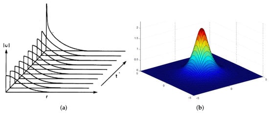
Figure 1.
(a) Development of the collapse of the 2D Townes soliton, shown in its radial cross-section. (b) The full spatial profile of the same soliton in the stationary state (source: https://www2.mathematik.uni-halle.de/dohnal/SOLIT_WAVES/NLS_blowup.pdf) Accessed on 29 June 2022.
As concerns 2D and 3D solitons with embedded vorticity (alias vortex rings, VRs), they are subject to the annular modulational instability, which develops faster than the collapse, leading to spontaneous splitting of the VR into two or several fragments, which are close to the corresponding fundamental (zero-vorticity) solitons. The exact number of the fragments is determined by the integer winding number (vorticity) carried by the VR, as shown in Figure 2. At a later stage of the evolution, the secondary solitons are destroyed by the collapse. In particular, vorticity-carrying varieties of the (unstable) 2D TSs were introduced in the works by [18,19,20].
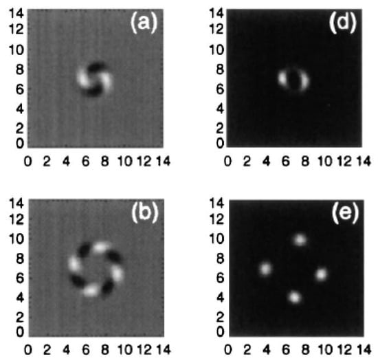
Figure 2.
Spontaneous splitting of unstable 2D VRs (vortex rings) with winding numbers (panels (a,d)) and (b,e) into fundamental (zero-vorticity) solitons (panel (c) is not included). Panels (a,b) display the real part of the complex wave function of the initial VRs, while (d,e) show the intensity distribution in the fragments produced by the splitting. These results were produced by simulations of the 2D NLS equations with saturable, rather than cubic, self-focusing nonlinearity, which stabilizes zero-vorticity solitons against the collapse, but does not stabilize the VRs against the splitting. Note that the total angular momentum is conserved, as the spin momentum of the initial VR is transformed into the orbital momentum of the emerging fragments [21]).
While the NLS equation with the self-attractive nonlinearity is a relevant model for many physical realizations in optics [22], BEC [23], physics of Langmuir waves in plasmas [24], etc., the occurrence of the collapse implies that these physical settings cannot be used for the straightforward creation of multidimensional solitons. Therefore, a cardinal problem is the search for physically realistic multidimensional systems that include additional ingredients that make it possible to suppress the collapse and help to predict and create stable (or maybe metastable) 2D and 3D solitons, see reviews by [25,26,27,28,29], and a new book by Malomed [30]. This can be done in various physical setups. In particular, stable 2D and 3D optical solitons can be predicted, and, eventually, experimentally created, if the optical medium features, in addition to the cubic self-focusing, higher-order quintic self-defocusing, which arrests the blowup, and thus provides the stabilization of 2D and 3D optical solitons. The creation of fundamental 2D solitons stabilized by the quintic self-defocusing was reported in the experiment by Falcão Filho et al. [31], and transitionally stable vortex solitons in the same medium were observed by Reyna et al. [32]. On the other hand, creation of stable 3D solitons remains a challenging problem.
Another extremely interesting option is to consider a binary BEC with the collapse driven by the attractive cubic interaction between its two intrinsically self-repulsive components. In this system, the collapse is arrested by a higher-order quartic self-repulsive term, which is induced in each component by the correction to the cubic mean-field interaction, induced by quantum fluctuations (the effect was first addressed in the classical work by [33]. As a result, the binary BEC creates completely stable 3D and quasi-2D self-trapped “quantum droplets” (QDs), which seem as multidimensional solitons (even if they are not usually called “solitons”, as the name of QDs is preferred in the literature). The prediction of QDs by Petrov [34] and Petrov and Astrakharchik [35] was quickly realized experimentally [36,37,38,39,40]. The existence of stable QDs with embedded vorticity was predicted as well [41,42], but such donut-shaped vortex tori have not yet been created in the experiment.
As concerns 2D and 3D settings with the purely cubic nonlinearity, it was predicted that completely stable 2D solitons can be created in two-component systems with the spin-orbit coupling (SOC) between the components [43,44]. Moreover, SOC may also create metastable solitons (ones that are stable against small perturbations, while the supercritical collapse remains possible) in the full 3D version of the same two-component system [45]. Due to the specific form of the SOC, both 2D and 3D two-component solitons maintained by this linear interaction between the components take the shape of semi-vortices, i.e., complexes including a zero-vorticity soliton in one component and a vortical one in the other, or mixed modes, in which zero-vorticity and vorticity-carrying terms are mixed in both components. In addition to that, stable 3D solitons may be supported by a combination of SOC, taken in the reduced 2D form, with the Zeeman splitting between the two components of the BEC [46]. Stable complexes of coupled 2D solitons can be supported by spatially periodic modulation of the local SOC strength [47].
All the above-mentioned mechanisms provide stabilization of 2D and 3D solitons in models with local nonlinear self- and cross-interactions in the single- and multi-component systems, respectively. On the other hand, a straightforward possibility is to use nonlocal nonlinearities for the stabilization of multidimensional localized states. First of all, it is evident that a fixed spatial scale (correlation length) of the nonlinear interaction arrests the development of the collapse, preventing the creation of the singularity with a vanishingly small intrinsic scale. Because the onset of the collapse is the basic mechanism leading to the instability of solitons in 2D and 3D spaces, the nonlocality may be a powerful method providing for the stabilization of such solitons. The present article offers a review of some selected results produced by the work performed in this direction. These are, chiefly, theoretical predictions, but some experimental findings are presented too.
Solitons are also well-known states in 1D models with nonlocal nonlinearity (Krolikowski and Bang, 2000). Although 1D solitons are not considered in this article in detail, it is relevant to mention the Benjamin–Ono equation [48,49], which was derived as a modification of the KdV equation for internal waves in stratified fluids, featuring nonlocal dispersion (i.e., the nonlocality appears in the linear part of the equation). This is an integrable equation which, similar to its KdV counterpart, admits exact multi-soliton solutions [50,51].
The review is not designed to be a comprehensive one, as otherwise it would grow into a full-size book. Particular topics selected for the inclusion in the review correspond to items that are singled out in the table of contents. Some of them represent themes and results that are well known from previous works, therefore they are briefly outlined in the review. Settings which were elaborated recently (especially those addressed in Section 3, produced by a 2D model for a binary BEC whose components are resonantly coupled by the interaction with a microwave electromagnetic field) are presented here in a more detailed form. Some topics that are not included in the review are mentioned in the concluding section.
1.1. Established Models: Thermal and Liquid-Crystal (Orientational) Nonlinearities in Optics
The possibility to stabilize multidimensional solitons in models with nonlocal nonlinear terms is well known. One of the first predictions of this stabilization mechanism for 2D solitons was published by Turitsyn [52]. Later, this topic was elaborated in detail theoretically, see a review by Krolikowski et al. [53]. In optics, the nonlocal propagation is realized in media with thermal nonlinearity, which originates form the local variation of the refractive index due to heating the medium by the propagating light. The corresponding model is based on the linear equation for the paraxial propagation of optical amplitude along the z axis, with transverse coordinates , which is coupled to the equation for the local perturbation of the refractive index, :
In Equation (2), term represents the local source of heating, and is the characteristic correlation length of the nonlocal interaction (in the limit of , the nonlocal nonlinear system is sometimes replaced by a linear Schrödinger equation, with the harmonic-oscillator potential, whose strength is proportional to the norm of the wave field—the so-called model of “accessible solitons” [54].
The basic model for nonlinear light propagation in nematic liquid crystals amounts to a system of equations that is similar to Equations (1) and (2), also leading to the creation of stable 2D solitons [55,56,57,58]. In that case, the nonlinearity is orientational, related to rotation of long molecules in the optical field.
The system of Equations (1) and (2) can be reduced to a single nonlocal NLS equation,
where G is the Green’s function of the linear operator
In many works, the Green’s function is approximately replaced by a Gaussian kernel:
The full system of Equations (1) and (2) and the single Equation (3) with the simplified kernel (5) produce quite similar results [59].
A 3D NLS equation for the spatiotemporal propagation of light in an ionized medium, with the cubic term, which is nonlocal in the temporal coordinate, thus representing the intra-pulse Raman shift, was introduced by Khalyapin and Bugay [60]. The equation also includes the third-order group-velocity dispersion, but does not include absorption of light. In the framework of this model, stable propagation of axially symmetric “light bullets” (as spatiotemporal solitons were named by Silberberg [61] was predicted, using the approximation based on the method of moments. In this context, the full 3D NLS equation was replaced by a system of evolution equations for seven integral moments.
In addition to straightforward stabilization of fundamental solitons, it was found that the nonlocal model provides for the existence of stable solitons with embedded vorticity, alias VRs (vortex rings), as well as higher-order VRs with a multiple-ring transverse structure [62,63,64]. The same model predicts 2D soliton complexes in the form of rotating dipoles [65]. A stability domain of vortex solitons was also found in a model of the light propagation in liquid crystals, where the nonlinearity is nonlocal too [66]. Therefore, the nonlocality is a promising method for the stabilization of complex 2D states. On the other hand, in the 3D version of the nonlocal system, produced by adding term to Equation (1), where t is the temporal coordinate, only fundamental 3D solitons are stable, while VRs are not ([67]). In addition to vortex solitons, robust necklace-shaped patterns in a nonlocal medium, produced by instability development of the solitary vortices, were explored by Walasik [68].
In the experiment, the formation of stable 2D fundamental solitons by light beams propagating through a vapor of hot sodium atoms, which is an effectively nonlocal optical medium, was demonstrated by Suter and Blasberg [69]. In liquid crystals, 2D solitons, which are often called “nematicons”, were created by Peccianti [70]. Then, as illustrated by Figure 3, stable optical VRs and elliptically deformed fundamental 2D solitons were created by Rotschild [71] in the lead glass, whose nonlocal nonlinearity is adequately modeled by Equations (1) and (2). Stable vortex solitons of higher orders—in particular, with vorticity (Zhang et al. [72]) and (Zhang, Zhou, and Dai [73])—were experimentally demonstrated in glasses with the thermal nonlocal nonlinearity. Stable vector (two-component) optical vortex solitons in a liquid-crystal medium were demonstrated byIzdebskaya, Assanto, and Krolikowski [74].
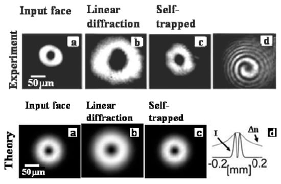
Figure 3.
Experimentally demonstrated creation of stable optical vortex solitons (with winding number ) supported by the nonlocal nonlinearity in the bulk waveguide made of lead glass. The top row demonstrates the intensity distribution in the input vortex beam (a), its linear diffraction when the power is insufficient to make the propagation nonlinear (b), and the formation of the stable vortex soliton when the power is sufficient for that (c). Panel (d) in the top row displays the experimentally observed phase distribution in the vortex. Panels (a–c) in the bottom row show the findings for the intensity distribution as produced, for the same setup, by simulations of Equations (1) and (2). In addition to that, panel (d) in the bottom row displays the distribution of the local intensity, , and local perturbation of the refractive index, n (here denoted n), in the cross-section of the vortex soliton, as produced by the numerical solution [71].
Another experiment with the propagation of (2 + 1) optical beams in an isotropic glass waveguide with the thermal nonlocal nonlinearity, and respective simulations of Equation (3), were performed by Zhang et al. [75]. They considered beams with an elliptical transverse shape. If the elliptically deformed beam did not carry angular momentum, it performed shape oscillations, similar to those demonstrated in simulations of the evolution of an elliptic ring kinks in the two-dimensional SG equation ([76]). On the other hand, a similar input to which angular momentum was imparted could self-trap into a stably rotating elliptic soliton, which resembles the so-called “propeller modes” [77].
1.2. A New Model with Linear Nonlocality: Fractional Diffraction in 2D
The introduction of fractional calculus in NLS equations has drawn much interest since it was proposed by Laskin [78]—originally, in the linear form—as the quantum-mechanical model, derived from the Feynman-integral formulation for particles moving by Lévy flights (see also the book by Laskin [79]). Then, realization of the effective fractional diffraction in optical cavities was proposed by Longhi [80] and by Zhang et al. [45]. Implementation of fractional linear Schrödinger equations in condensed-matter settings has been reported by Stickler [81] and by Pinsker et al. [82].
The nonlinearity was added to the fractional Schrödinger equations, starting from the work by Secchi and Squassima [83]. In terms of the realization of the fractional diffraction in optics, the cubic self-focusing represents the Kerr nonlinearity of the material of the waveguide. The cubic nonlinearity also makes sense if added to the original fractional Schrödinger equation in quantum mechanics. The so extended fractional model may be considered as an effective Gross–Pitaevskii (GP) equation for the gas of quantum particles moving by Lévy flights. The fractional NLS equations give rise to many theoretical results for solitons in the framework of the fractional NLS equations, see a brief review of the topic by Malomed [84]. In particular, the 2D fractional NLS equation for amplitude of the optical wave propagating along the z direction, under the action of an effective transverse potential, , and the usual cubic self-focusing, is written as
The fractionality of the diffraction operator in Equation (6) is determined by the Lévy index (LI), . In usually considered models, it takes values in interval
corresponding to the usual NLS equation. Equation (6) reduces to the 1D form by dropping coordinate y, which leads to the following equation
The affinity of Equations (6) and (8) to nonlocal models, although with linear nonlocality, is demonstrated by the definition of the fractional derivative in Equation (8), and the fractional-diffraction operator in Equation (6):
These integral expressions are produced, essentially, as juxtapositions of the direct and inverse Fourier transform for field . In fact, there are many different definitions of fractional derivatives; the one adopted in Equation (9), which is relevant to the above-mentioned physical realizations in quantum mechanics and optics, is often called the Riesz derivative [85,86]. It is relevant to mention that alternative definitions of the fractional derivatives, such as Caputo and Riemann–Liouville ones, may also produce solitons in the framework of the fractional NLS equation [87,88], although the use of those definitions in the context of optics models is less straightforward.
An essential problem posed by the fractional NLS Equations (6) and (8), which include the cubic self-focusing term, is the possibility of the onset of collapse in it. Well-known criteria for the occurrence of the supercritical and critical collapse for the usual NLS equations [12,13,14] can be easily generalized for the fractional NLS Equations (6) and (8) with the cubic self-focusing. The derivation is based on the analysis of scaling of the fractional-diffraction and self-focusing terms, and in the energy (Hamiltonian) of the equation, assuming spontaneous self-compression of the wave-function configuration towards the limit of the zero spatial scale, , under the condition of the conservation of the integral norm, . The latter condition implies that the squared amplitude of the wave function scales as , where and 2 for Equations (6) and (8), respectively. With regard to this result, the conclusions for the scaling are and . The collapse cannot develop if grows at faster than . Thus, the conclusion is that the critical and supercritical collapse takes place, severally, at LI values
In other words, in the case of the 1D fractional Equation (8), the critical collapse takes place at , and does not occur at . In the 2D fractional model based on Equation (6), the collapse takes place in the entire interval (7): critical at (which is tantamount to the usual 2D NLS equation with the cubic self-focusing), and supercritical at .
The occurrence of the collapse makes it difficult to obtain stable solitons as solutions of Equation (6). Nevertheless, stable 2D solitons, including ones with embedded vorticity, were predicted, adding the self-defocusing quintic term to the model ([89,90]), or replacing the local cubic self-focusing by its nonlocal counterpart, the same as in Equations (3) and (5). A trapping harmonic-oscillator potential in Equation (6), , may also provide stabilization of 2D solitons at ([84]). The latter result is similar to the well-known one for the usual two-dimensional NLS/GP equation, which corresponds to in Equation (6). Further, a similar fractional model with a double-well potential gives rise to 2D solitons with spontaneously broken symmetry [91].
2. Anisotropic Quasi-2D Solitons Built by Dipole-Dipole Interactions (DDIs) in BEC of Magnetic Atoms
An important example of nonlocal nonlinearity is provided by the DDI of magnetic atoms in BEC composed of such atoms [92]. The corresponding GP equation, for the mean-field wave function , includes both the local nonlinearity, with strength g, which represents contact collisions between atoms, and the nonlocal DDI, with strength . In the scaled form, the GP equation is
where z is the direction in which atomic magnetic moments are polarized by an external magnetic field, stands for the 3D integration, and is an external potential acting on the condensate. In terms of physical units, and , where is the scattering length of the atomic collisions, N is the number of atoms in the condensate, is a characteristic spatial scale, is the vacuum permeability, m is the atomic mass, and is the atomic magnetic moment.
Stable 3D solitons in the free space () cannot be supported by the DDI. A possibility is to create quasi-2D (pancake-shaped) solitons, applying the confining potential acting in a particular direction. The simplest configuration of that type is an axially symmetric one, with the potential applied along the same axis, z, along which the polarizing field is directed. However, self-trapping of the wave function in this configuration is impossible because the interaction between parallel magnetic dipoles is repulsive. On the other hand, it was predicted by Giovanazzi, Görlitz, and Pfau [93] that the sign of the DDI may be effectively reversed, replacing in Equation (12), by means of an additional ac magnetic field which drives fast rotation of the dipoles (a similar prediction for polar molecules carrying electric dipole moments was made by Micheli et al. [94]). In the framework of this setup, stable solitons were predicted by Pedri and Santos [95], and stable vortex solitons with winding number were predicted by Tikhonenkov, Malomed, and Vardi [96].
A more challenging objective is to search for stable quasi-2D solitons, supported by the DDI proper, with the magnetic moments polarized perpendicular to the confinement direction, or at an angle to it, as shown schematically in Figure 4 (the notation for the Cartesian coordinates in this figure is different from that in Equation (12)).
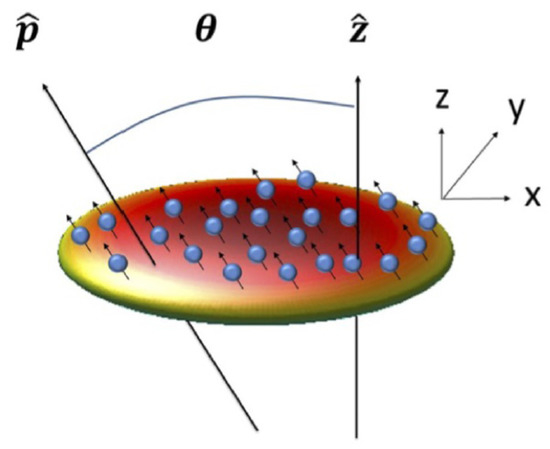
Figure 4.
A scheme for the creation of quasi-2D (“pancake-shaped”) solitons supported by the DDI of magnetic atoms confined in the vertical direction by the trapping harmonic-oscillator potential. The angle between the fixed orientation of atomic magnetic dipoles, , and the confinement direction is [97].
An approach to the solution of this problem was elaborated by Tikhonenkov, Malomed, and Vardi [98], assuming that the confinement was imposed in the direction of y by the harmonic-oscillator potential
in Equation (12) (i.e., indeed, the confinement direction is perpendicular to the polarizing magnetic field). The consideration started with the VA, based on an anisotropic Gaussian ansatz for the 3D wave function,
supplemented by the normalization condition,
Ansatz (14) was inserted in the energy (Hamiltonian) corresponding to Equation (12), with the confining potential (13) (i.e., the atomic magnetic dipoles are polarized along axis z, and the atoms are located close to the plane:
The substitution of ansatz (14) and calculation of the integrals yields
where
Then, values of the variational parameters , , in ansatz (14) are predicted by the energy-minimization condition,
Detailed analysis of Equation (22) has demonstrated that, under condition
it yields a minimum of energy (19), which may predict the existence of stable solitons as solutions to Equation (12). The meaning of constraint (23) is that, naturally, stable solitons cannot exist if the DDI is not strong enough.
Direct numerical solution of Equation (12) has produced stable solitons with shapes close to those predicted by the VA, see an example in Figure 5. The strongly anisotropic shape of the soliton is a natural manifestation of the anisotropic form of the DDI in Equation (12).
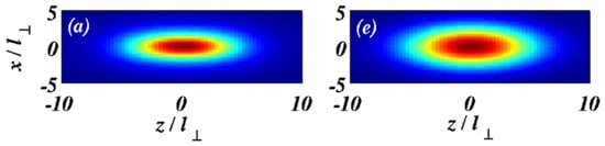
Figure 5.
The The left panel, (a): the density distribution in a stable quasi-2D (pancake-shaped) soliton solution of Equation (12) in the mid plane, , for parameters and (which satisfies condition (23)). The right panel, (e): the same, as predicted by the VA solution based on ansatz (14) [98]. Intermediate panels (b,c,d) are not included.
Because the polarization of the atomic magnetic moments in the plane is determined by the orientation of the external magnetic field, it is also interesting to explore a dynamical state in which the field slowly rotates in this plane (perpendicular to the confinement direction, y). The dynamics can be simulated using the GP Equation (12), in which the DDI term is written in the rotating coordinates,
The simulations have demonstrated that the stable pancake-shaped soliton is able to adiabatically follow the rotation of the polarizing field, provided that the angular velocity in Equation (24) is small enough, as shown in Figure 6. Faster rotation leads to deformation of the soliton.
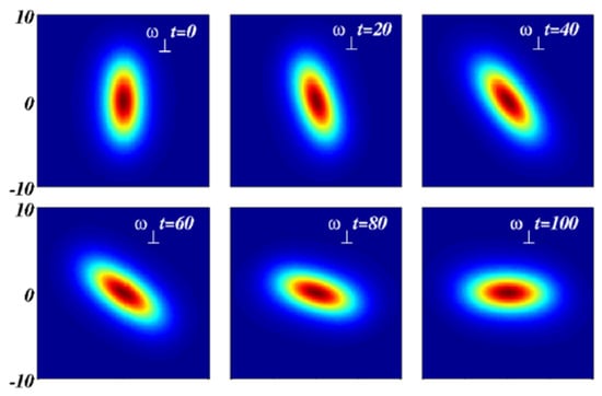
Figure 6.
Stable counter-clockwise rotation of the pancake-shaped soliton (the same whose static shape is shown in Figure 5), following the rotation of the coordinates as per Equation (24) with angular velocity . Shown are snapshots of the density distribution in the mid plane, produced by simulations of Equation (12) at moments of times indicated in the panels [98].
An experimentally realistic scenario for the creation of the stable pancake-shaped solitons was elaborated byKöberle et al. [99]. The scenario includes temporal variation of the scattering length and strength of the trapping potential, with the purpose to help building the soliton from an experimentally available input. Also included were additional physically significant factors, such as three-body losses and random fluctuations of the scattering length.
A similar, but more general, quasi-2D setting, under the action of the confining potential (13) with the tilt angle in Figure 4, was considered by Chen et al. [97]. Using a combination of VA and numerical solution of the accordingly modified Equation (12), it was found that stable pancake-shaped solitons with the anisotropic shape persist in an interval of the tilt angles
The limit value in Equation (25) depends on parameters, always staying close to the so-called magic angle,
The meaning of this angle is that the potential of the DDI for two parallel point-like dipoles, with angle between the line of length R connecting them and the common direction of the magnetic moments, is proportional to
Thus, potential (27) vanishes at .
Equation (12) with potential (13) keeps the Galilean invariance in the plane, which suggests to set the anisotropic solitons in motion in this plane, and simulate collisions between them [100]. The simulations demonstrate that the collisions may be deeply inelastic, leading to merger of the colliding solitons into a single quasi-soliton state [101].
Recently, a 3D spatiotemporal model similar to Equation (12) was derived by [102] Zhao et al. (2022) for a two-component model of a gas of Rydberg atoms with long-range interactions in an optical medium with electromagnetically-induced transparency. The model produces stable 3D fundamental solitons, as well as stable solitons with embedded vorticity. A protocol for storage and retrieval of the 3D solitons in this system was elaborated too.
3. Giant Vortex Rings (VRs) in Microwave-Coupled Binary BEC
Photonic tools, such as optical-lattice and trapping potentials, are broadly used in the experimental and theoretical work with single- and multi-component BECs. In particular, microwave (MW) fields are used to resonantly couple different atomic states that form two-component condensates [103,104]. In many cases, the feedback of the BEC on the MW fields is ignored. Nevertheless, the feedback produced by relatively dense condensates may induce field-mediated long-range interaction in BEC, which is often called the local-field effect (LFE) and gives rise to significant phenomena. In particular, the LFE acting on the electric component of the field explains asymmetric matter-wave diffraction [105,106] and predicts polaritonic solitons in soft optical lattices [107]. Further, the resonant coupling of the magnetic components of the MW field to the condensate of two-level atoms opens the way to the creation of hybrid microwave-matter-wave solitons [108]. In fact, the MW-mediated long-range interaction may cover the whole condensate, in contrast with fast-decaying nonlocal interactions in optics and dipolar BEC (cf. Equations (3), (5) and (12)).
In the 2D configuration, a hybrid system including a pseudo-spinor BEC matter-wave function, whose two components are coupled by the MW field, as shown schematically in Figure 7, was introduced by Qin, Dong, and Malomed [109]. As shown below, stable solitons in the form of VRs, with arbitrarily large values of winding number S, readily self-trap in this 2D setting. The conclusion remains valid if the system includes the local repulsive or attractive interaction. In particular, the domain in which the VRs remain stable against the critical collapse, driven by the local attraction between the components, expands with the increase of S, persisting for arbitrarily high values of S. This conclusion is remarkable, as, in other systems which admit stable VRs with , their stability domain shrinks with the increase of S. In this sense, the VRs predicted in the 2D hybrid matter-wave-microwave system may be considered as stable giant vortices, because large values of S naturally imply a large radius of the ring.
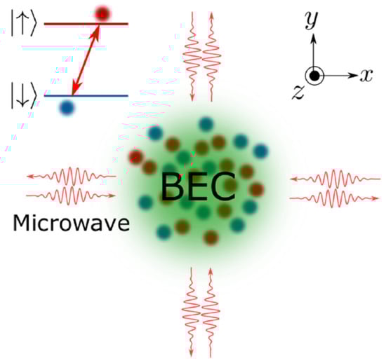
Figure 7.
The scheme of the 2D hybrid system that builds giant VRs. The pseudo-spinor (two-component) wave function represents two atomic states coupled by the MW (microwave) field, as shown in the figure. The MW field is polarized in the direction perpendicular to the system’s plane [109].
3.1. The Model
Following Figure 7, a nearly-2D binary BEC, composed of two different atomic states, is described by the pseudo-spinor wave function, , with each component emulating “spin-up” and “spin-down” states of the usual spinor. In the scaled notation (setting the Planck’s constant, atomic mass, vacuum magnetic permeability, and the absolute value of the magnetic moment to be 1), the corresponding atomic Hamiltonian is
where and are the 2D momentum and magnetic moment, is detuning of the MW from the transition between the atomic states and , is the Pauli matrix, and
is the magnetic induction, with magnetic field and magnetization . Assuming that the atomic magnetic moments are polarized along the field, the field and magnetization may be taken in the scalar form. Then, in the rotating-wave approximation the components of the wave function obey the following system of coupled GP equations:
Here ∗ stands for the complex conjugate, is the strength of the MW-atom coupling, and the strength of the cross-interaction of the two components is determined by the scalar product of the matrix elements of the magnetic moment: .
The magnetic field is determined by the inhomogeneous Helmholtz equation. In the present notation, it is
where k is the MW wavenumber. As the respective wavelength of the MW field, , is always much greater than an experimentally relevant size of the BEC, the second term in Equation (32) may be omitted in comparison with the first term, reducing Equation (32) to the Poisson equation:
Because the medium’s magnetization, which is the source of the magnetic field, is concentrated in the nearly-2D “pancake”, the Poisson equation may be treated as a two-dimensional one. Then, using the Green’s function of the 2D Poisson equation, the magnetic field is produced by Equation (33) as
where is the set of the coordinates in the 2D plane. The substitution of expression (34) in GP Equations (30) and (31) casts them in the form of coupled NLS equations with the nonlocal interaction, cf. Equations (3) and (12), acting along with the local cross-interaction with strength :
Equations (35) and (36) are supplemented by the normalization condition,
If collisions between atoms belonging to the two components are considered (with the corresponding strength of the contact interaction made tunable, in the experiment, by means of the Feshbach resonance), the additional cross-interaction terms can be absorbed into rescaled coefficient in Equations (35) and (36). Collisions may also give rise to self-interaction terms, and , in the parentheses of Equations (35) and (36), respectively. Note also that the same Equations (35) and (36) (without the self-interaction terms) apply to a different physical setting, viz., a degenerate Fermi gas with spin , in which and represent two spin components, coupled by the MW magnetic field [108,110].
The following analysis chiefly addresses the symmetric (zero-detuning) system, which corresponds to in Equations (35) and (36). Then, these equations coalesce into a single one for ,
and normalization (37) reduces to
In this case, the above-mentioned self-interaction coefficient, , may be absorbed into .
The remaining scaling invariance of Equation (38) makes it possible to finally fix . In physical units, assuming the transverse-confinement size m and MW wavelength ∼1 mm, the typical solutions for VR solitons presented below correspond to “heavy” BECs with the number of atoms , which are available in the experiment [111,112], a typical VR radius being ∼10 m.
3.2. Results
In polar coordinates , stationary solutions to Equation (38) with chemical potential and integer vorticity S are looked for as
where is a real radial wave function, which satisfies the following equation, obtained by the substitution of ansatz (40) in Equation (38):
The form of the nonlocal term in Equation (41) was derived by explicitly performing the angular integration in the last term of Equation (38). The corresponding magnetic field is then produced by performing the integration with respect to the angular coordinate in Equation (34):
Characteristic examples of solutions for , produced by the imaginary-time simulations of Equation (38), along with the corresponding profiles of , are displayed in Figure 8, for different values of S and . Numerical results demonstrate that the fundamental solitons, which correspond to , and VRs with are destroyed by the collapse at , see Table 1. This critical value of the coefficient of the inter-component attraction can be found by considering the energy corresponding to Equation (38),
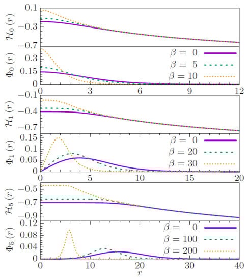
Figure 8.
Numerically found radial wave function (defined as per Equation (40)) and the corresponding magnetic field, , calculated as per Equation (34). Top panels: the fundamental solitons (); middle panels: stable VRs with ; bottom panels: stable higher-order VRs (). All the solutions pertain to indicated values of strength of the inter-component attraction, and [109].

Table 1.
and : numerically obtained and analytically predicted values of the strength of the local nonlinearity, , up to which the 2D fundamental solitons (with ) and VRs (vortex rings, with and 2) exist. : the numerically identified stability boundary of the VRs. Numerical data are produced by Equations (35), (36), and (41) [109].
The numerical findings demonstrate that, for and when is large enough, the vortex soliton is shaped as a narrow ring, see Figure 8. It may be approximated by the usual quasi-1D soliton shape in the radial direction (cf. the approximation which was used, in the 2D NLS equation with the CQ nonlinearity, by Caplan et al. [113]:
where R is the VR’s radius, and normalization (39) is taken into regard. Then, the substitution of approximation (43) in Equation (42) yields
Radius R of the soliton’s ring is selected as a value corresponding to the energy minimum, , i.e.,
In comparison with numerical results, Equation (45) provides a reasonable approximation for the radius of narrow VRs. Then, the above-mentioned critical value is analytically (“”) predicted as one at which vanishes, i.e., the ring collapses to the center,
As seen in Table 1, this approximate result is very close to its numerically found counterparts at , and is quite close for as well.
A remarkable fact is that the analytical prediction (46) does not depend on strength of the nonlocal interaction, hence it also predicts the onset of the collapse in the usual 2D cubic NLS equation, corresponding to :
Recall that the collapse-onset threshold for the solutions of Equation (47) with is determined by the TS norm, [12,13,14], which, in the present notation (taking into account normalization (39)), implies
The analytical expression (46) is not relevant for , but the data displayed in Table 1 demonstrate that Equation (46) offers an approximate analytical solution for the long-standing problem of the prediction of the collapse threshold for the VR solutions of Equation (47). In the numerical form, critical values which are tantamount to were found, for , by Kruglov, Logvin, and Volkov [18]. However, an analytical approximation for them was not available prior to the results reported by Qin, Dong, and Malomed [109].
The independence of with all values of S on is an exact property of Equation (38). To explain it, note that, at the final stage of the collapse, when the shrinking VR becomes extremely narrow, the equation for the wave function is asymptotically equivalent to the simplified Equation (47), as the nonlocal term in Equation (38) is negligible in this limit. Therefore, the condition for the onset of the collapse is identical in both equations, (38) and (47). However, the difference between them is that the 2D cubic NLS Equation (47) gives rise to soliton solutions (which are TSs, both fundamental or vortical ones), solely at , and they are completely unstable. On the other hand, the LFE-induced long-range interaction in Equation (38) helps to create fundamental solitons and VRs with all values of S at , and the crucially important difference is that a part of these solution families are stable, see below.
The stability of the solitons was systematically investigated by real-time simulations of Equation (38) with small random perturbations added to the stationary solutions (furthermore, the full system of coupled Equations (35) and (36) with independent random perturbations added to components and , was also simulated, to test the stability against breaking the symmetry between them). The fundamental solitons () are stable in their entire existence region, .
The simulations of the evolution of the VR families reveal an internal stability boundary, (see Table 1), the vortices being stable at
In the interval of , the VRs are broken by azimuthal perturbations into rotating necklace-shaped sets of fragments, which resembles the initial stage of the instability development of vortex solitons in usual models. However, unlike those models, in the present case the necklace does not expand, remaining confined under the action of the effective nonlocal interaction. Typical examples of the stable and unstable evolution of VRs are displayed in Figure 9.
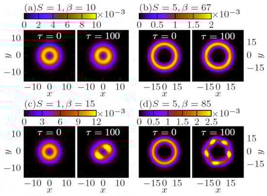
Figure 9.
The top and bottom panels display several examples of the stable and unstable perturbed evolution of the VRs with indicated values of S and . The initial shape of the VR () is compared to the output produced by the simulations of Equation (38) with at (here, replaces t). The necklace-shaped pattern, produced by the instability in the right bottom panel, remains confined (keeping the original overall radius) in the course of the subsequent evolution [109].
To address the stability of the VRs against azimuthal perturbations analytically, one can approximate the wave function of a perturbed (azimuthally modulated) VR by
This ansatz is substituted in Equation (38), and an effective evolution equation for the modulation amplitude A is derived by averaging in the radial direction:
In the framework of Equation (51), straightforward analysis of the modulational stability of the solution with against perturbations with integer winding numbers p shows that the stability is sustained under the threshold condition,
Further, the numerical results demonstrate that, similar to what is known in other models [32,114,115,116], the critical instability corresponds to (for instance, the appearance of five fragments in the part of Figure 9 corresponding to demonstrates that, for , the dominant splitting mode indeed has ). Thus, the analytical prediction is that the VRs remain stable if satisfies condition (52), i.e., at
(note that Equation (53) does not include , being universal, in this sense). On the other hand, the numerically found stability limits collected in Table 1 obey an empirical formula,
The inference is that the analytical approximation (53) is quite accurate for .
The implication of Equations (46), (53), and (54) is that the giant VRs, with large values of S, are much more robust than their counterparts with smaller S. As mentioned above, this counter-intuitive feature is opposite to what was previously found in those models, which are able to produce stable VRs with [32,115,116,117,118,119,120]. It is relevant to stress that, at , the fundamental soliton () is the system’s ground state, while, at , the ground state does not exist, due to the possibility of the collapse. The vortices with cannot represent the ground state, but, nevertheless, they exist as metastable ones, cf. the above-mentioned result for metastable 3D solitons in the SOC system which exist while the system does not have a ground state, due to the presence of the supercritical collapse [45].
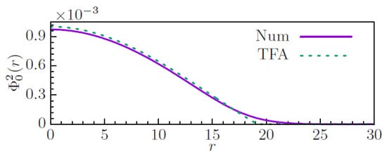
In the case of the strong repulsive local interaction, which corresponds to a large positive coefficient in Equation (38), solitons with can be constructed by means of the Thomas–Fermi (TF) approximation. In this case, instead of using the Green’s function, it is more convenient to apply the TF approximation directly to Equations (30) and (31), in which the kinetic-energy terms are dropped, while is kept in the Poisson Equation (33). The corresponding result is
where , is the first zero of Bessel function , and is a normalization constant. Figure 10 shows that the TF approximation agrees very well with the numerical solution.
3.3. Self-Accelerating 2D Vortex Rings (VRs)
In the studies of diverse nonlinear-wave systems, much interest was drawn to states which can exhibit self-accelerating and/or self-bending motion. A well-known example is provided by Airy waves, which were predicted by Berry and Balazs [121] as an exact solution of the 1D linear Schrödinger equation. Using the similarity of the linear Schrödinger equation to the paraxial wave-propagation equation in classical physics, this concept was transferred to many areas of classical and semi-classical phenomenology, including optics [122], plasmonics [123], BEC [124], acoustics [125], gas discharge [126], electron beams [127], and studies of surface waves in hydrodynamics [128].
Ideal Airy waves, with slowly decaying one-sided oscillatory tails, carry an infinite norm, which makes them unphysical objects. The problem was resolved by using truncated Airy waves with a finite norm [122,129]. However, the truncation leads to gradual degradation of the self-accelerating wave packets. Another caveat is that, while Airy waves are eigenmodes of linear media, nonlinearity causes their deformation and destruction, as studied in detail in various settings [130,131,132,133,134,135].
On the other hand, the nonlinearity of the medium, which tends to destroy Airy waves, can be used, instead, to create well-localized eigenmodes, which are able to move with self-acceleration, remaining robust objects. In addition to their stability in the presence of the nonlinearity, an asset of such modes is that they do not develop extended tails, hence their naturally defined norm is convergent. In particular, it was predicted by Batz and Peschel [136] and experimentally demonstrated by Wimmer et al. [137] that two pulses subject to the action of the group-velocity dispersion with opposite signs may form a self-accelerating bound state in a photonic-crystal fiber. This is possible because the pulses may be considered as quasi-particles with opposite signs of the effective mass, hence the opposite forces of the interaction between the pulses drive both of them with identical signs of the acceleration. For solitons, a similar possibility was elaborated by Sakaguchi and Malomed [138], in a system of nonlinearly coupled GP equations with an optical-lattice potential, where solitons with positive and negative effective masses (it is well known that the effective mass may be negative for gap solitons) form stable self-accelerating pairs.
Continuing the work in this direction, it was shown by Qin et al. [139] that the GP-Poisson system, based on Equations (30), (31), and (33), admits exact realization of accelerating motion of 2D solitons. In this case, Equations (30) and (31) may also include the above-mentioned self-interaction terms , but the Poisson equation should not include the term , which is present in the Helmholtz Equation (32). Thus, the relevant system is
The system is characterized by its energy (Hamiltonian),
The result reported by Qin et al. [139] is that Equations (56)–(58) are exactly invariant with respect to transformation from the quiescent reference frame into a non-inertial one, which moves, in the 2D plane , with vectorial acceleration , combined with an additional constant velocity . The coordinates, wave functions, and magnetic field in the traveling frame are defined as
In fact, Equations (60)–(63) are a generalization of the usual Galilean boost for the accelerating reference frame.
According to Equations (60) and (61), coordinates of the center of the stable 2D soliton (which may be the fundamental one of VR) moves as
Equation (64) represents a curvilinear trajectory in the 2D plane: at small t, it is close to a straight line with slope , while at it is asymptotically close to a line with a different slope, . In particular, in the case of , the trajectory is a parabola:
Note that the solution of the 2D Poisson Equation (58) for the quiescent soliton has the standard asymptotic form far from the region where the source of the field is located:
cf. Equation (34’). The difference of the magnetic-field component (63) of the self-accelerating 2D soliton from its quiescent counterpart (66) is the presence of the terms linear in x and y, which implies that the accelerating motion is maintained by the properly built background magnetic field.
The analytical results are corroborated by Figure 11, which displays numerical findings for moving VRs, produced by simulations of Equations (56)–(58). These solutions demonstrate exactly the same self-accelerating motion of the robust VRs as predicted by Equation (65), in cases when the underlying system does not or does contain the local nonlinear terms.
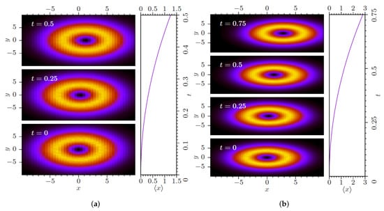
Figure 11.
(a) The plot of for a stable self-accelerating VR with , , (see Equations (60) and (61)), produced by numerical solution of Equations (56)–(58) with (no local nonlinearity) and . The right panel shows the time dependence of coordinate x of the VR’s center. (b) The same as in (a), but for in Equations (56) and (57) [139].
4. Conclusions
To keep the length of this review within reasonable limits, only a few topics have been selected for a relatively detailed presentation. These topics are sufficiently novel ones, while well-known results for 2D solitons stabilized with the help of spatial nonlocality were reviewed in earlier publications (in particular, by Krolikowski et al. [53]; Khoo [56]; Assanto et al. [57]; Peccianto and Assanto [58]).
As concerns other aspects of this broad area, it is relevant to mention, in particular, the theoretical and experimental results that demonstrate the creation of stable three-dimensional QDs in single-component BECs with DDIs between atoms carrying permanent magnetic moments [140,141,142]. A possibility of the creation of QDs with embedded vorticity in this setting was analyzed by Cidrim et al. [143], with a conclusion that such states are completely unstable (on the contrary to the above-mentioned prediction of stable 3D and 2D vortical QDs in the two-component BEC with contact inter-atomic interactions by Kartashov et al. [41] and Li et al. [42]).
A related finding is the prediction by Gligorić et al. [144] of stable 2D solitons maintained by DDIs in a discrete system, which may be realized by the dipolar BEC loaded into a deep optical-lattice potential. It was also predicted by Li et al. [145] that the DDIs, acting along with SOC in a two-component BEC, can maintain stable 2D gap solitons, in the case when the kinetic energy is negligible in comparison to the SOC energy in this system.
As for development of the work on the topic of multidimensional (chiefly, two-dimensional) solitons in nonlocal media, an interesting direction may be the study of interactions between such solitons, and the possible formation of their bound states. It is natural to expect that the nonlocality gives rise to effective long-range interactions between far separated solitons, making the situation essentially different from multidimensional settings based on local nonlinearities, where only short-range soliton–soliton interactions were predicted [146]. In particular, the long-range interactions may affect symmetries of the emerging bound states of multidimensional solitons. Another relevant direction is to develop the analysis for dissipative 2D solitons in media combining nonlocal nonlinearity, gain, and loss. Systems of this type may naturally occur in nonlinear optics.
Funding
This research received no external funding.
Institutional Review Board Statement
Not applicable.
Informed Consent Statement
Not applicable.
Data Availability Statement
Not applicable.
Acknowledgments
I would like to thank Branko Dragović for the invitation to submit this paper to the special issue of journal Symmetry on the topic of “Advances in nonlinear dynamics and symmetries”. This work was supported, in part, by the Israel Science Foundation through grant No. 1286/17.
Conflicts of Interest
The author declares no conflict of interest.
References
- Manton, N.; Sutcliffe, P. Topological Solitons; Cambridge University Press: Cambridge, UK, 2004. [Google Scholar]
- Radu, E.; Volkov, M.S. Stationary ring solitons in field theory: Knots and vortons. Phys. Rep. 2008, 468, 101–151. [Google Scholar] [CrossRef]
- Ablowitz, M.J.; Segur, H. Solitons and the Inverse Scattering Transform; SIAM: Philadelphia, PA, USA, 1981. [Google Scholar]
- Newell, A. Solitons in Mathematics and Physics; SIAM: Philadelphia, PA, USA, 1985. [Google Scholar]
- Zakharov, V.E.; Manakov, S.V.; Novikov, S.P.; Pitaevskii, L. Theory of Solitons: The Inverse Problem Method; Nauka Publishers: Moscow, Russia, 1980; English translation: Consultants Bureau: New York, NY, USA, 1984. [Google Scholar]
- Biondini, G.; Pelinovsky, D. Kadomtsev-Petviashvili equation. Scholarpedia 2008, 3, 6539. [Google Scholar] [CrossRef]
- Manakov, S.V.; Zakharov, V.E.; Bordag, L.A.; Its, A.; Matveev, V.B. Two-dimensional solitons of the Kadomtsev-Petviashvili equation and their interaction. Phys. Lett. A 1977, 63, 205–206. [Google Scholar] [CrossRef]
- Yang, J. Nonlinear Waves in Integrable and Nonintegrable Systems; SIAM: Philadelphia, PA, USA, 2010. [Google Scholar]
- Desaix, M.; Anderson, D.; Lisak, M. Variational approach to collapse of optical pulses. J. Opt. Soc. Am. B 1991, 8, 2082–2086. [Google Scholar] [CrossRef]
- Chiao, R.Y.; Garmire, E.; Townes, C.H. Self-trapping of optical beams. Phys. Rev. Lett. 1964, 13, 479–482. [Google Scholar] [CrossRef]
- Bradley, C.C.; Sackett, C.A.; Tollett, J.J.; Hulet, R.G. Evidence of Bose-Einstein condensation in an atomic gas with attractive interactions. Phys. Rev. Lett. 1995, 75, 1687–1690, Erratum in: Phys. Rev. Lett. 1997, 79, 1170. [Google Scholar] [CrossRef]
- Bergé, L. Wave collapse in physics: Principles and applications to light and plasma waves. Phys. Rep. 1998, 303, 259–370. [Google Scholar] [CrossRef]
- Fibich, G. The Nonlinear Schrödinger Equation: Singular Solutions and Optical Collapse; Springer: Berlin/Heidelberg, Germany, 2015. [Google Scholar]
- Sulem, C.; Sulem, P.-L. The Nonlinear Schrödinger Equation: Self-Focusing and Wave Collapse; Springer: New York, NY, USA, 1999. [Google Scholar]
- Zabusky, N.J.; Kruskal, M.D. Interaction of “solitons” in a collisional plasma and the recurrence of initial states. Phys. Rev. Lett. 1965, 15, 240–243. [Google Scholar] [CrossRef]
- Chen, C.-A.; Hung, C.-L. Observation of universal quench dynamics and Townes soliton formation from modulational instability in two-dimensional Bose gases. Phys. Rev. Lett. 2020, 125, 250401. [Google Scholar] [CrossRef]
- Chen, C.-A.; Hung, C.-L. Observation of scale invariance in two-dimensional matter-wave Townes solitons. Phys. Rev. Lett. 2021, 127, 023604. [Google Scholar]
- Kruglov, V.I.; Logvin, Y.A.; Volkov, V.M. The theory of spiral laser beams in nonlinear media. J. Mod. Phys. 1992, 39, 2277–2291. [Google Scholar] [CrossRef]
- Kruglov, V.I.; Vlasov, R.A. Spiral self-trapping propagation of optical beams. Phys. Lett. A 1985, 111, 401–404. [Google Scholar] [CrossRef]
- Kruglov, V.I.; Volkov, V.M.; Vlasov, R.A.; Drits, V.V. Auto-waveguide propagation and the collapse of spiral light beams in non-linear media. J. Phys. A Math. Gen. 1988, 21, 4381–4395. [Google Scholar] [CrossRef]
- Firth, W.J.; Skryabin, D.V. Optical solitons carrying orbital angular momentum. Phys. Rev. Lett. 1997, 79, 2450–2453. [Google Scholar] [CrossRef]
- Kivshar, Y.S.; Agrawal, G.P. Optical Solitons: From Fibers to Photonic Crystals; Academic Press: San Diego, CA, USA, 2003. [Google Scholar]
- Pitaevskii, L.P.; Stringari, S. Bose-Einstein Condensation; Oxford University Press: Oxford, UK, 2003. [Google Scholar]
- Schochet, S.H.; Weinstein, M.I. The nonlinear Schrödinger limit of the Zakharov equations governing Langmuir turbulence. Commun. Math. Phys. 1986, 106, 569–580. [Google Scholar] [CrossRef]
- Malomed, B.A. Multidimensional solitons: Well-established results and novel findings. Eur. Phys. J. Spec. Top. 2016, 225, 2507–2532. [Google Scholar] [CrossRef]
- Malomed, B.A. (INVITED) Vortex solitons: Old results and new perspectives. Phys. D 2019, 399, 108–137. [Google Scholar] [CrossRef]
- Malomed, B.A.; Mihalache, D.; Wise, F.; Torner, L. Spatiotemporal optical solitons. J. Opt. B Quant. Semicl. Opt. 2005, 7, R53–R72. [Google Scholar]
- Malomed, B.A.; Mihalache, D.; Wise, F.; Torner, L. Viewpoint: On multidimensional solitons and their legacy in contemporary atomic, molecular and optical physics. J. Phys. At. Mol. Opt. Phys. 2016, 49, 170502. [Google Scholar]
- Kartashov, Y.; Astrakharchik, G.; Malomed, B.; Torner, L. Frontiers in multidimensional self-trapping of nonlinear fields and matter. Nat. Rev. Phys. 2019, 1, 185–197. [Google Scholar] [CrossRef]
- Malomed, B.A. Multidimensional Solitons; American Institute of Physics: University Park, MD, USA, 2022. [Google Scholar]
- Falcão-Filho, L.; de Araújo, C.B.; Boudebs, G.; Leblond, H.; Skarka, V. Robust two-dimensional spatial solitons in liquid carbon disulfide. Phys. Rev. Lett. 2013, 110, 013901. [Google Scholar] [CrossRef] [PubMed]
- Reyna, A.S.; Boudebs, G.; Malomed, B.A.; de Araújo, C.B. Robust self-trapping of vortex beams in a saturable optical medium. Phys. Rev. A 2016, 93, 013840. [Google Scholar] [CrossRef]
- Lee, T.D.; Huang, K.; Yang, C.N. Eigenvalues and eigenfunctions of a Bose system of hard spheres and its low temperature properties. Phys. Rev. 1957, 106, 1135–1145. [Google Scholar] [CrossRef]
- Petrov, D.S. Quantum mechanical stabilization of a collapsing Bose-Bose mixture. Phys. Rev. Lett. 2015, 115, 155302. [Google Scholar] [CrossRef]
- Petrov, D.S.; Astrakharchik, G.E. Ultradilute low-dimensional liquids. Phys. Rev. Lett. 2016, 117, 100401. [Google Scholar] [CrossRef]
- Cabrera, C.; Tanzi, L.; Sanz, J.; Naylor, B.; Thomas, P.; Cheiney, P.; Tarruell, L. Quantum liquid droplets in a mixture of Bose-Einstein condensates. Science 2018, 359, 301–304. [Google Scholar] [CrossRef]
- Cheiney, P.; Cabrera, C.R.; Sanz, J.; Naylor, B.; Tanzi, L.; Tarruell, L. Bright soliton to quantum droplet transition in a mixture of Bose-Einstein condensates. Phys. Rev. Lett. 2018, 120, 135301. [Google Scholar] [CrossRef]
- D’Errico, C.; Burchianti, A.; Prevedelli, M.; Salasnich, L.; Ancilotto, F.; Modugno, M.; Minardi, F.; Fort, C. Observation of quantum droplets in a heteronuclear bosonic mixture. Phys. Rev. Res. 2019, 1, 033155. [Google Scholar] [CrossRef]
- Ferioli, G.; Semeghini, G.; Masi, L.; Giusti, G.; Modugno, G.; Inguscio, M.; Gallem, A.; Recati, A.; Fattori, M. Collisions of self-bound quantum droplets. Phys. Rev. Lett. 2019, 122, 090401. [Google Scholar] [CrossRef]
- Semeghini, G.; Ferioli, G.; Masi, L.; Mazzinghi, C.; Wolswijk, L.; Minardi, F.; Modugno, M.; Modugno, G.; Inguscio, M.; Fattori, M. Self-bound quantum droplets of atomic mixtures in free space? Phys. Rev. Lett. 2018, 120, 235301. [Google Scholar] [CrossRef]
- Kartashov, Y.V.; Malomed, B.A.; Tarruell, L.; Torner, L. Three-dimensional droplets of swirling superfluids. Phys. Rev. A 2018, 98, 013612. [Google Scholar] [CrossRef]
- Li, Y.; Chen, Z.; Luo, Z.; Huang, C.; Tan, H.; Pang, W.; Malomed, B.A. Two-dimensional vortex quantum droplets. Phys. Rev. A 2018, 98, 063602. [Google Scholar] [CrossRef]
- Sakaguchi, H.; Li, B.; Malomed, B.A. Creation of two-dimensional composite solitons in spin-orbit-coupled self-attractive Bose-Einstein condensates in free space. Phys. Rev. E 2014, 89, 032920. [Google Scholar] [CrossRef]
- Sakaguchi, H.; Sherman, E.Y.; Malomed, B.A. Vortex solitons in two-dimensional spin-orbit coupled Bose-Einstein condensates: Effects of the Rashba-Dresselhaus coupling and the Zeeman splitting. Phys. Rev. E 2016, 94, 032202. [Google Scholar] [CrossRef]
- Zhang, Y.; Liu, X.; Belić, M.R.; Zhong, W.; Zhang, Y.; Xiao, M. Propagation dynamics of a light beam in a fractional Schrödinger equation. Phys. Rev. Lett. 2015, 115, 180403. [Google Scholar] [CrossRef]
- Kartashov, Y.V.; Torner, L.; Modugno, M.; Sherman, E.Y.; Malomed, B.A.; Konotop, V.V. Multidimensional hybrid Bose-Einstein condensates stabilized by lower-dimensional spin-orbit coupling. Phys. Rev. Res. 2020, 2, 013036. [Google Scholar] [CrossRef]
- Kartashov, Y.V.; Sherman, E.Y.; Malomed, B.A.; Konotop, V.V. Stable two-dimensional soliton complexes in Bose–Einstein condensates with helicoidal spin–orbit coupling. New J. Phys. 2020, 22, 103914. [Google Scholar] [CrossRef]
- Benjamin, T. Internal waves of permanent form in fluids of great depth. J. Fluid Mech. 1967, 29, 559–592. [Google Scholar] [CrossRef]
- Ono, H. Algebraic solitary waves in stratified fluids. J. Phys. Soc. Jpn. 1975, 39, 1082–1091. [Google Scholar]
- Fokas, A.S.; Ablowitz, M.J. The inverse scattering transform for the Benjamin-Ono equation, a pivot for multidimensional problems. Stud. Appl. Math. 1983, 68, 1–10. [Google Scholar]
- Kaup, D.; Matsuno, Y. The inverse scattering for the Benjamin-Ono equation. Stud. Appl. Math. 1998, 101, 73–98. [Google Scholar] [CrossRef]
- Turitsyn, S.K. Spatial dispersion of nonlinearity and stability of multidimensional solitons. Theor. Math. Phys. 1985, 64, 797–801. [Google Scholar] [CrossRef]
- Królikowski, W.; Bang, O.; Nikolov, N.I.; Neshev, D.; Wyller, J.; Rasmussen, J.J.; Edmundson, D. Modulational instability, solitons and beam propagation in spatially nonlocal nonlinear media. J. Opt. B Quantum Semiclass. Opt. 2004, 6, S288–S294. [Google Scholar] [CrossRef]
- Snyder, A.W.; Mitchell, D.J. Accessible solitons. Science 1997, 276, 1538–1541. [Google Scholar] [CrossRef]
- Minzoni, A.A.; Smyth, N.F.; Worthy, A.L. Modulation solutions for nematicon propagation in nonlocal liquid crystals. J. Opt. Soc. Am. B 2007, 24, 1549–1556. [Google Scholar] [CrossRef]
- Khoo, I.C. Nonlinear optics of liquid crystalline materials. Phys. Rep. 2009, 471, 221–267. [Google Scholar] [CrossRef]
- Assanto, G.; Karpierz, M.A. Nematicons: Self-localised beams in nematic liquid crystals. Liq. Cryst. 2009, 36, 1161–1172. [Google Scholar] [CrossRef]
- Peccianti, M.; Assanto, G. Nematicons. Phys. Rep. 2012, 516, 147–208. [Google Scholar] [CrossRef]
- Wyller, J.; Królikowski, W.; Bang, O.; Rasmussen, J.J. Generic features of modulational instability in nonlocal Kerr media. Phys. Rev. E 2002, 66, 066615. [Google Scholar] [CrossRef]
- Khalyapin, V.A.; Bugay, A.N. Analytical study of light bullets stabilization in the ionized medium. Chaos Sol. Fract. 2022, 156, 111799. [Google Scholar] [CrossRef]
- Silberberg, Y. Collapse of optical pulses. Opt. Lett. 1990, 15, 1282–1284. [Google Scholar] [CrossRef] [PubMed]
- Briedis, D.; Petersen, D.E.; Edmundson, D.; Krolikowski, W.; Bang, O. Ring vortex solitons in nonlocal nonlinear media. Opt. Exp. 2005, 13, 435–443. [Google Scholar] [CrossRef] [PubMed]
- Skupin, S.; Bang, O.; Edmundson, D.; Krolikowski, W. Stability of two-dimensional spatial solitons in nonlocal nonlinear media. Phys. Rev. E 2006, 73, 066603. [Google Scholar] [CrossRef] [PubMed]
- Yakimenko, A.I.; Zaliznyak, Y.A.; Kivshar, Y. Stable vortex solitons in nonlocal self-focusing nonlinear media. Phys. Rev. E 2005, 71, 065603(R). [Google Scholar] [CrossRef]
- Lopez-Aguayo, S.; Desyatnikov, A.S.; Kivshar, Y.S.; Skupin, S.; Królikowski, W.; Bang, O. Stable rotating dipole solitons in nonlocal optical media. Opt. Lett. 2006, 31, 1100–1102. [Google Scholar] [CrossRef]
- Jung, P.S.; Izdebskaya, Y.V.; Shvedov, V.G.; Christodoulides, D.; Krolikowski, W. Formation and stability of vortex solitons in nematic liquid crystals. Opt. Lett. 2021, 46, 62–65. [Google Scholar] [CrossRef]
- Mihalache, D.; Mazilu, D.; Lederer, F.; Malomed, B.A.; Kartashov, Y.V.; Crasovan, L.-C.; Torner, L. Three-dimensional spatiotemporal optical solitons in nonlocal nonlinear media. Phys. Rev. E 2006, 73, 025601(R). [Google Scholar] [CrossRef]
- Walasik, W.; Silahli, S.Z.; Litchinitser, N. Dynamics of necklace beams in nonlinear colloidal suspensions. Sci. Rep. 2017, 7, 11709. [Google Scholar] [CrossRef]
- Suter, D.; Blasberg, T. Stabilization of transverse solitary waves by a nonlocal response of the nonlinear medium. Phys. Rev. A 1993, 48, 4583–4587. [Google Scholar] [CrossRef]
- Peccianti, M.; Assanto, G.; Luca, A.D.; Umeton, C.; Khoo, I.C. Electrically assisted self-confinement and waveguiding in planar nematic liquid crystal cells. Appl. Phys. Lett. 2000, 77, 7–9. [Google Scholar] [CrossRef]
- Rotschild, C.; Cohen, O.; Manela, O.; Segev, M.; Carmon, T. Solitons in nonlinear media with an infinite range of nonlocality: First observation of coherent elliptic solitons and of vortex-ring solitons. Phys. Rev. Lett. 2005, 95, 213904. [Google Scholar] [CrossRef]
- Zhang, H.; Chen, M.; Yang, L.; Tian, B.; Chen, C.; Guo, Q.; Shou, Q.; Hu, W. Higher-charge vortex solitons and vector vortex solitons in strongly nonlocal media. Opt. Lett. 2019, 44, 3098–3101. [Google Scholar] [CrossRef]
- Zhang, H.; Zhou, T.; Dai, C. Stabilization of higher-order vortex solitons by means of nonlocal nonlinearity. Phys. Rev. A 2022, 105, 013520. [Google Scholar] [CrossRef]
- Izdebskaya, Y.; Assanto, G.; Krokikovski, W. Observation of stable-vector vortex solitons. Opt. Lett. 2015, 40, 4182–4184. [Google Scholar] [CrossRef]
- Zhang, H.; Zhou, T.; Shou, Q.; Guo, Q. Optical elliptic breathers in isotropic nonlocal nonlinear media. Opt. Exp. 2022, 30, 9336–9347. [Google Scholar] [CrossRef]
- Christiansen, P.L.; Grønbech-Jensen, N.; Lomdahl, P.S.; Malomed, B.A. Oscillations of eccentric pulsons. Phys. Scr. 1997, 55, 131–134. [Google Scholar] [CrossRef]
- Carmon, T.; Uzdin, R.; Pigier, C.; Musslimani, Z.H.; Segev, M.; Nepomnyashchy, A. Rotating propeller solitons. Phys. Rev. Lett. 2001, 87, 143901. [Google Scholar] [CrossRef]
- Laskin, N. Fractional quantum mechanics and Lévy path integrals. Phys. Lett. A 2000, 268, 298–305. [Google Scholar] [CrossRef]
- Laskin, N. Fractional Quantum Mechanics; World Scientific: Singapore, 2018. [Google Scholar]
- Longhi, S. Fractional Schrödinger equation in optics. Opt. Lett. 2015, 40, 1117–1120. [Google Scholar] [CrossRef]
- Stickler, B.A. Potential condensed-matter realization of space-fractional quantum mechanics: The one-dimensional Lévy crystal. Phys. Rev. E 2013, 88, 012120. [Google Scholar] [CrossRef]
- Pinsker, F.; Bao, W.; Zhang, Y.; Ohadi, H.; Dreismann, A.; Baumberg, J.J. Fractional quantum mechanics in polariton condensates with velocity-dependent mass. Phys. Rev. B 2015, 92, 195310. [Google Scholar] [CrossRef]
- Secchi, S.; Squassina, M. Soliton dynamics for fractional Schrödinger equations. Appl. Anal. 2014, 93, 1702–1729. [Google Scholar] [CrossRef]
- Malomed, B.A. Optical solitons and vortices in fractional media: A mini-review of recent results. Photonics 2021, 8, 353. [Google Scholar] [CrossRef]
- Agrawal, O.P. Fractional variational calculus in terms of Riesz fractional derivatives. J. Phys. A Math. Theor. 2007, 40, 6287–6303. [Google Scholar] [CrossRef]
- Cai, M.; Li, C.P. On Riesz derivative. Fract. Calc. Appl. Anal. 2019, 22, 287–301. [Google Scholar] [CrossRef]
- Kwasnicki, M. Ten equivalent definitions of the fractional Laplace operators. Fract. Calc. Appl. Anal. 2017, 20, 7–51. [Google Scholar] [CrossRef]
- Navickas, Z.; Telksnys, T.; Marcinkevicius, R.; Ragulskis, M. Operator-based approach for the construction of analytical soliton solutions to nonlinear fractional-order differential equations. Chaos Solitons Fractals 2017, 104, 625–634. [Google Scholar] [CrossRef]
- Li, P.; Malomed, B.A.; Mihalache, D. Vortexsolitons in fractional nonlinear Schrödinger equation with the cubic-quintic nonlinearity. Chaos Solitons Fract. 2020, 137, 109783. [Google Scholar]
- Li, P.; Malomed, B.A.; Mihalache, D. Metastablesoliton necklaces supported by fractional diffraction and competing nonlinearities. Opt. Exp. 2020, 28, 34472–34488. [Google Scholar]
- Li, P.; Li, R.; Dai, C. Existence, symmetry breaking bifurcation and stability of two-dimensional optical solitons supported by fractional diffraction. Opt. Exp. 2021, 29, 3193–3210. [Google Scholar] [CrossRef] [PubMed]
- Lahaye, T.; Menotti, C.; Santos, L.; Lewenstein, M.; Pfau, T. The physics of dipolar bosonic quantum gases. Rep. Prog. Phys. 2009, 72, 126401. [Google Scholar] [CrossRef]
- Giovanazzi, S.; Görlitz, A.; Pfau, T. Tuning the dipolar interaction in quantum gases. Phys. Rev. Lett. 2003, 89, 130401. [Google Scholar] [CrossRef]
- Micheli, A.; Pupillo, G.; Büchler, H.P.; Zoller, P. Cold polar molecules in two-dimensional traps: Tailoring interactions with external fields for novel quantum phases. Phys. Rev. A 2007, 76, 043604. [Google Scholar] [CrossRef]
- Pedri, P.; Santos, L. Two-dimensional bright solitons in dipolar Bose-Einstein condensates. Phys. Rev. Lett. 2005, 95, 200404. [Google Scholar] [CrossRef]
- Tikhonenkov, I.; Malomed, B.A.; Vardi, A. Vortex solitons in dipolar Bose-Einstein condensates. Phys. Rev. A 2008, 78, 043614. [Google Scholar] [CrossRef]
- Chen, X.-Y.; Chuang, Y.-L.; Lin, C.-Y.; Wu, C.-M.; Li, Y.; Malomed, B.A.; Lee, R.-K. Magic tilt angle for stabilizing two-dimensional solitons by dipole-dipole interactions. Phys. Rev. A 2017, 96, 043631. [Google Scholar]
- Tikhonenkov, I.; Malomed, B.A.; Vardi, A. Anisotropic solitons in dipolar Bose-Einstein condensates. Phys. Rev. Lett. 2008, 100, 090406. [Google Scholar] [CrossRef]
- Köberle, P.; Zajec, D.; Wunner, G.; Malomed, B.A. Creating two-dimensional bright solitons in dipolar Bose-Einstein condensates. Phys. Rev. A 2012, 85, 023630. [Google Scholar] [CrossRef]
- Eichler, R.; Zajec, D.; Köberle, P.; Main, J.; Wunner, G. Collisions of anisotropic two-dimensional bright solitons in dipolar Bose-Einstein condensates. Phys. Rev. A 2012, 86, 053611. [Google Scholar]
- Young-S, L.E.; Adhikari, S.K. Deep inelastic collision of two-dimensional anisotropic dipolar condensate solitons. Comm. Nonlin. Sci. Num. Sim. 2022, 106, 106094. [Google Scholar]
- Zhao, Y.; Lei, Y.-B.; Xu, Y.-X.; Xu, S.-L.; Triki, H.; Biswas, A.; Zhou, Q. Vector spatiotemporal solitons and their memory features in cold Rydberg gases. Chin. Phys. Lett. 2022, 39, 034202. [Google Scholar] [CrossRef]
- Burnett, B.R.J.K.; Scott, T.F. Theory of an output coupler for Bose-Einstein condensed atoms. Phys. Rev. Lett. 1997, 78, 1607–1611. [Google Scholar]
- Bookjans, E.M.; Vinit, A.; Raman, C. Quantum Phase Transition in an Antiferromagnetic Spinor Bose-Einstein Condensate. Phys. Rev. Lett. 2011, 107, 195306. [Google Scholar] [CrossRef]
- Li, K.; Deng, L.; Hagley, E.W.; Payne, M.G.; Zhan, M.S. Matter-wave self-imaging by atomic center-of-mass motion induced interference. Phys. Rev. Lett. 2008, 101, 250401. [Google Scholar] [CrossRef]
- Zhu, J.; Dong, G.; Shneider, M.N.; Zhang, W. Strong local-field effect on the dynamics of a dilute atomic gas irradiated by two counterpropagating optical fields: Beyond standard optical lattices. Phys. Rev. Lett. 2011, 106, 210403. [Google Scholar] [CrossRef]
- Dong, G.; Zhu, J.; Zhang, W.; Malomed, B.A. Photon-atomic solitons in a Bose-Einstein condensate trapped in a soft optical lattice. Phys. Rev. Lett. 2013, 110, 250401. [Google Scholar] [CrossRef]
- Qin, J.; Dong, G.; Malomed, B.A. Hybrid matter-wave-microwave solitons produced by the local-field effect. Phys. Rev. Lett. 2015, 115, 023901. [Google Scholar] [CrossRef]
- Qin, J.; Dong, G.; Malomed, B.A. Stable giant vortex annuli in microwave-coupled atomic condensates. Phys. Rev. A 2016, 94, 053611. [Google Scholar] [CrossRef]
- Radzihovsky, L.; Sheehy, D.E. Imbalanced Feshbach-resonant Fermi gases. Rep. Prog. Phys. 2010, 73, 076501. [Google Scholar] [CrossRef]
- Comparat, D.; Fioretti, A.; Stern, G.; Dimova, E.; Tolra, B.; Pillet, P. Optimized production of large Bose-Einstein condensates. Phys. Rev. A 2006, 73, 043410. [Google Scholar] [CrossRef]
- van der Stam, K.M.R.; van Ooijen, E.D.; Meppelink, R.; Vogels, J.M.; van der Straten, P. Large atom number Bose-Einstein condensate of sodium. Rev. Sci. Instr. 2007, 78, 013102. [Google Scholar] [CrossRef]
- Caplan, R.M.; Carretero-Gonzalez, R.; Kevrekidis, P.G.; Malomed, B.A. Existence, stability, and scattering of bright vortices in the cubic-quintic nonlinear Schrödinger equation. Math. Comput. Simul. 2012, 82, 1150–1171. [Google Scholar] [CrossRef]
- Brtka, M.; Gammal, A.; Malomed, B.A. Hidden vorticity in binary Bose-Einstein condensates. Phys. Rev. A 2010, 82, 053610. [Google Scholar] [CrossRef]
- Pego, R.L.; Warchall, H.A. Spectrally stable encapsulated vortices for nonlinear Schrödinger equations. J. Nonlinear Sci. 2002, 12, 347–394. [Google Scholar] [CrossRef]
- Quiroga-Teixeiro, M.; Michinel, H. Stable azimuthal stationary state in quintic nonlinear optical media. J. Opt. Soc. Am. B 1997, 14, 2004–2009. [Google Scholar] [CrossRef]
- Borovkova, O.V.; Kartashov, Y.V.; Malomed, B.A.; Torner, L. Algebraic bright and vortex solitons in defocusing media. Opt. Lett. 2011, 36, 3088–3090. [Google Scholar] [CrossRef]
- Borovkova, O.V.; Kartashov, Y.V.; Torner, L.; Malomed, B.A. Bright solitons from defocusing nonlinearities. Phys. Rev. E 2011, 84, 035602(R). [Google Scholar] [CrossRef]
- Driben, R.; Kartashov, Y.V.; Malomed, B.A.; Meier, T.; Torner, L. Soliton gyroscopes in media with spatially growing repulsive nonlinearity. Phys. Rev. Lett. 2014, 112, 020404. [Google Scholar] [CrossRef]
- Sudharsan, J.B.; Radha, R.; Fabrelli, H.; Gammal, A.; Malomed, B.A. Stable multiple vortices in collisionally inhomogeneous attractive Bose-Einstein condensates. Phys. Rev. A 2015, 92, 053601. [Google Scholar] [CrossRef]
- Berry, M.V.; Balazs, N.L. Nonspreading wave packets. Am. J. Phys. 1979, 47, 264–267. [Google Scholar] [CrossRef]
- Siviloglou, G.A.; Christodoulides, D.N. Accelerating finite energy Airy beams. Opt. Lett. 2007, 32, 979–981. [Google Scholar] [CrossRef]
- Minovich, A.E.; Klein, A.E.; Neshev, D.N.; Pertsch, T.; Kivshar, Y.S.; Christodoulides, D.N. Airy plasmons: Non-diffracting optical surface waves. Laser Photonics Rev. 2013, 8, 221–232. [Google Scholar] [CrossRef]
- Efremidis, N.K.; Paltoglou, V.; von Klitzing, W. Accelerating and abruptly autofocusing matter waves. Phys. Rev. A 2013, 87, 043637. [Google Scholar] [CrossRef]
- Zhang, P.; Li, T.; Zhu, J.; Zhu, X.; Yang, S.; Wang, Y.; Yin, X.; Zhang, X. Generation of acoustic self-bending and bottle beams by phase engineering. Nat. Commun. 2014, 5, 4316. [Google Scholar] [CrossRef]
- Clerici, M.; Hu, Y.; Lassonde, P.; Milian, C.; Couairon, A.; Christodoulides, D.N.; Chen, Z.; Razzari, L.; Vidal, F.; Legare, F.; et al. Laser-assisted guiding of electric discharges around objects. Sci. Adv. 2015, 1, e1400111. [Google Scholar] [CrossRef]
- Voloch-Bloch, N.; Lereah, Y.; Lilach, Y.; Gover, A.; Arie, A. Generation of electron Airy beams. Nature 2013, 494, 331–335. [Google Scholar] [CrossRef]
- Fu, S.; Tsur, Y.; Zhou, J.; Shemer, L.; Arie, A. Propagation dynamics of Airy water-wave pulses. Phys. Rev. Lett. 2015, 115, 034501. [Google Scholar] [CrossRef]
- Siviloglou, G.A.; Broky, J.; Dogariu, A.; Christodoulides, D.N. Observation of accelerating Airy beams. Phys. Rev. Lett. 2007, 99, 213901. [Google Scholar] [CrossRef]
- Ellenbogen, T.; Voloch-Bloch, N.; Ganany-Padowicz, A.; Arie, A. Nonlinear generation and manipulation of Airy beams. Nat. Photonics 2009, 3, 395–398. [Google Scholar] [CrossRef]
- Jia, S.; Lee, J.; Fleischer, J.W.; Siviloglou, G.A.; Christodoulides, D.N. Diffusion-trapped Airy beams in photorefractive media. Phys. Rev. Lett. 2010, 104, 253904. [Google Scholar] [CrossRef]
- Hu, Y.; Huang, S.; Zhang, P.; Lou, C.; Xu, J.; Chen, Z. Persistence and breakdown of Airy beams driven by an initial nonlinearity. Opt. Lett. 2010, 35, 3952–3954. [Google Scholar] [CrossRef]
- Kaminer, I.; Segev, M.; Christodoulides, D.N. Self-accelerating self-trapped optical beams. Phys. Rev. Lett. 2011, 106, 213903. [Google Scholar] [CrossRef]
- Lotti, A.; Faccio, D.; Couairon, A.; Papazoglou, D.G.; Panagiotopoulos, P.; Abdollahpour, D.; Tzortzakis, S. Stationary nonlinear Airy beams. Phys. Rev. A 2011, 84, 021807. [Google Scholar] [CrossRef]
- Fattal, Y.; Rudnick, A.; Marom, D.M. Soliton shedding from Airy pulses in Kerr media. Opt. Exp. 2011, 18, 17298–17307. [Google Scholar] [CrossRef]
- Batz, S.; Peschel, U. Diametrically driven self-accelerating pulses in a photonic crystal fiber. Phys. Rev. Lett. 2013, 110, 193901. [Google Scholar] [CrossRef]
- Wimmer, M.; Regensburger, A.; Bersch, C.; Miri, M.-A.; Batz, S.; Onishchukov, G.; Christodoulides, D.N.; Peschel, U. Optical diametric drive acceleration through action-reaction symmetry breaking. Nat. Phys. 2013, 9, 780–784. [Google Scholar] [CrossRef]
- Sakaguchi, H.; Malomed, B.A. Interactions of solitons with positive and negative masses: Shuttle motion and coacceleration. Phys. Rev. E 2019, 99, 022216. [Google Scholar] [CrossRef]
- Qin, J.; Liang, Z.; Malomed, B.A.; Dong, G. Tail-free self-accelerating solitons and vortices. Phys. Rev. A 2019, 99, 023610. [Google Scholar] [CrossRef]
- Chomaz, L.; Baier, S.; Petter, D.; Mark, M.J.; Wachtler, F.; Santos, L.; Ferlaino, F. Quantum-fluctuation-driven crossover from a dilute Bose-Einstein condensate to a macrodroplet in a dipolar quantum fluid. Phys. Rev. X 2016, 6, 041039. [Google Scholar] [CrossRef]
- Ferrier-Barbut, I.; Kadau, H.; Schmitt, M.; Wenzel, M.; Pfau, T. Observation of quantum droplets in a strongly dipolar Bose gas. Phys. Rev. Lett. 2016, 116, 215301. [Google Scholar] [CrossRef]
- Schmitt, M.; Wenzel, M.; Bottcher, F.; Ferrier-Barbut, I.; Pfau, T. Self-bound droplets of a dilute magnetic quantum liquid. Nature 2016, 539, 259–262. [Google Scholar] [CrossRef]
- Cidrim, A.; dos Santos, F.E.; Henn, E.A.; Macrí, T. Vortices in self-bound dipolar droplets. Phys. Rev. A 2018, 98, 023618. [Google Scholar] [CrossRef]
- Gligorić, G.; Maluckov, A.; Stepić, M.; Hadžievski, L.; Malomed, B.A. Two-dimensional discrete solitons in dipolar Bose-Einstein condensates. Phys. Rev. A 2010, 81, 013633. [Google Scholar] [CrossRef]
- Li, Y.; Liu, Y.; Fan, Z.; Pang, W.; Fu, S.; Malomed, B.A. Two-dimensional dipolar gap solitons in free space with spin-orbit coupling. Phys. Rev. A 2017, 95, 063613. [Google Scholar] [CrossRef]
- Malomed, B.A. Potential of interaction between two- and three-dimensional solitons. Phys. Rev. E 1998, 58, 7928–7933. [Google Scholar] [CrossRef]
Publisher’s Note: MDPI stays neutral with regard to jurisdictional claims in published maps and institutional affiliations. |
© 2022 by the author. Licensee MDPI, Basel, Switzerland. This article is an open access article distributed under the terms and conditions of the Creative Commons Attribution (CC BY) license (https://creativecommons.org/licenses/by/4.0/).