Analysis of Identified Particle Transverse Momentum Spectra Produced in pp, p–Pb and Pb–Pb Collisions at the LHC Using TP-like Function

Abstract

In the framework of a multi-source thermal model at the partonic level, we have analyzed transverse momentum spectra of hadrons measured by the ALICE Collaboration in proton–proton ($pp$ or p–p) collisions at the center-of-mass energy of $\sqrt{s}=7$ and 13 TeV, proton–lead (p–Pb) collisions at $\sqrt{s_{NN}}=5.02$ TeV, and lead–lead (Pb–Pb) collisions at $\sqrt{s_{NN}}=2.76$ TeV. For mesons (baryons), the contributions of two (three) constituent quarks are considered, in which each quark contributes to hadron transverse momentum to obey the revised phenomenological Tsallis transverse momentum distribution for Maxwell–Boltzmann particles (the TP-like function, in short) with isotropic random azimuthal angles. Three main parameters, namely, the revised index $a_0$, effective temperature T, and entropy-related index n, are obtained, showing the same tendency for both small and large systems with respect to the centrality (or multiplicity) of events, the rest mass of hadrons, and the constituent mass of quarks.

1. Introduction

The deconfined high-temperature and high-density state of nuclear matter, called quark–gluon plasma (QGP), is often studied by ultra-relativistic nuclear collisions. The transverse momentum ($p_T$) spectra and ratios of identified hadrons provide a means to study the properties of matter created in these collisions and the mechanism by which quasi-free partons are transformed into observable hadrons. The relative contributions of different hadronization mechanisms rely on the change of hadrons’ $p_T$. At low $p_T$ recombination may be dominant, while at high $p_T$ hadrons may originate from fragmentation processes. This mainly depends on the potential transverse momentum distribution of quarks. Therefore, it is important to have the $p_T$ spectra of identified mesons and baryons in a wide $p_T$ range.

Unlike the up (u) and down (d) quarks that form ordinary matter, strange (s) quarks do not exist in the form of valence quarks in the colliding species, and they are light enough to be produced in large quantities in the process of ultra-relativistic collisions. In the early state of high-energy collisions, strangeness is produced in hard (perturbative) $2\to 2$ partonic scattering processes by flavor creation ($gg\to s\overline{s}$, $q\overline{q}\to s\overline{s}$) and flavor excitation ($gs\to gs$, $qs\to qs$). In addition, strangeness is created during subsequent partonic evolution via the gluon-splitting process ($g\to s\overline{s}$). These processes tend to dominate the production of strange hadrons with high $p_T$, and the production of strange hadrons with low $p_T$ is mainly dominated by non-perturbative processes.

The production of strange hadrons is suppressed compared to that of hadrons containing only $u/d$ quarks because s quarks need higher threshold energy to be excited. In particle–particle collisions, the degree of suppression of strange hadrons is an important parameter in theoretical model-based analysis. Therefore, the measurement of strange hadron production imposes restrictions on the tuning of theoretical models. The study of strange and multi-strange particles in relativistic heavy-ion collisions is an important tool for exploring the properties of the systems governed by the strong interaction. The enhancement of strangeness in heavy-ion collisions is one of the most important signals of QGP [1,2,3]. The particle spectra provide abundant information about the temperature and collective flow of the system, which reflects the dynamics of kinetic freeze-out conditions. There are different definitions of the temperature; because it probably is not the standard temperature, the temperature in a particular distribution can be regarded as a parameter.

In the past decades, researchers searching for QGP have conducted extensive study of hadrons containing one or more s quarks [1,4,5]. However, the origin of the strangeness enhancement is not yet clear when strangeness is observed to be enhanced in proton–proton ($pp$ or p–p) collisions as well [6,7]. The azimuthal correlations and mass-dependent hardening of the $p_T$ spectra observed in the high-multiplicity $pp$ and proton–nucleus ($pA$ or p–A) collisions are typically attributed to the formation of strongly interacting quark–gluon media [1,8,9,10,11,12,13,14,15,16,17,18]. The abundance of strange particles at different center-of-mass energies is in accordance with the calculation of the thermal statistical model [19,20,21]. Strangeness, light flavor production, and heavy-ion collision dynamics provide evidence for the properties of the fluid-like behavior and collectivity of the medium [7,22]. Studying $pp$ collisions at high multiplicity is of considerable significance, as it opens up the possibility of understanding nuclear reaction phenomena from a microscopic perspective.

Studies of charged particles in high multiplicity $pp$ and proton–lead (p–Pb) collisions at the Large Hadron Collider (LHC) have shown striking similarities to lead–lead (Pb–Pb) collisions. The enhancement of (multi-)strange hadrons [11], azimuthal correlations and double-ridge structure [12,13], nonzero elliptic flow ($v_2$) coefficients and other anisotropic flow measurements [9,23,24,25,26,27], mass ordering in hadron $p_T$ spectra, and characteristic modifications of baryon to meson ratios [10] have shown that these phenomena collectively exist in small collision systems. In addition, in $pp$, p–Pb, and Pb–Pb collisions, the continuous evolution of the ratio of light-flavor hadrons to pions has shown a function of final state charged particle multiplicity density [24,28,29]. The observed similarities [30,31,32,33,34,35,36,37] indicate that there is a common underlying mechanism that determines the chemical composition of the systems produced in different collision systems with comparable final-state multiplicities. That is, underlying strong interactions in these collisions occurred among partons and not among nucleons.

We recently considered contributor quarks; based on the Tsallis statistics [38,39,40,41,42,43], the available $p_T$ spectra of various particles and jets produced in collisions of small systems ($pp$, deuteron–gold (d–Au), p–Pb) and large systems (gold–gold (Au–Au) and Pb–Pb) at high energies were studied [44,45,46] (where the term “contributor quark” is used instead of “constituent quark” due to the fact that “contributor quark” can refer to the production of leptons and jets as well) [44,46]. In our calculations, we used the convolution of two or three revised phenomenological Tsallis transverse momentum distributions for the Maxwell–Boltzmann particles (the TP-like function, in short) [47,48,49,50]. The application of convolution means that we have considered the azimuthal angles of contributor quarks to be the same or parallel to each other. A detailed consideration shows that the azimuthal angles (${\varphi }_1$ and ${\varphi }_2$) of contributor quarks may be isotropic and random. The special cases include cases parallel ($|{\varphi }_1-{\varphi }_2|=0$ or $\pi$) and perpendicular to each other ($|{\varphi }_1-{\varphi }_2|=\pi /2$). The analytical expressions for parallel and perpendicular cases are available. Any other cases use a Monte Carlo method, for which it is difficult to provide an analytical expression.

In the current work, we use a Monte Carlo method in the framework of a multi-source thermal model at the partonic level to study the $p_T$ spectra of identified hadrons produced in the collisions of different centralities (or multiplicities) with small systems ($pp$ and p–Pb) and a large system (Pb–Pb), including non-strange hadrons (${\pi }^{+}+{\pi }^{-}$ and $p+\overline{p}$), strange hadrons ($K^{+}+K^{-}$, $K_S^0$, $K^{*}+\overline{K}{}^{*}$, and $\mathsf{\Lambda }+\overline{\mathsf{\Lambda }}$), and multi-strange hadrons (${\mathsf{\Xi }}^{-}+\overline{\mathsf{\Xi }}{}^{+}$ and ${\mathsf{\Omega }}^{-}+\overline{\mathsf{\Omega }}{}^{+}$). The azimuthal angles of the contributor or constituent quarks are isotropic and random. The size of the transverse momentum of each quark contributing to a hadron’s $p_T$ is assumed to obey the TP-like function. Mathematically, we study the synthesis of two or three vectors with changeable azimuthal angles and sizes.

The $p_T$ spectra in a wide range can reflect more dynamical information on the collision process. In order to verify the feasibility of the model, extract relevant parameters, study the dependence of parameters on centrality, thereby and understand the mechanism of reactions at the partonic level at LHC-scale energies, we used data on the $p_T$ spectra of identified hadrons produced in $pp$ collisions at $\sqrt{s}=7$ and 13 TeV [28,51,52,53], p–Pb collisions at $\sqrt{s_{NN}}=5.02$ TeV [10,11,54,55], and Pb–Pb collisions at $\sqrt{s_{NN}}=2.76$ TeV [56,57,58,59] measured by the ALICE Collaboration.

The remainder of this paper is structured as follows. The formalism and method are described in Section 2. Results and discussion are provided in Section 3. In Section 4, we summarize our main observations and conclusions.

2. Formalism and Method

Inspired by the SU(3) super polymorphism theory, in 1964 Murray Gell-Mann proposed the quark model [60]. There are two commonly used masses of quarks. One is the current mass of a quark, which refers to the mass in the Lagrangian of quantum field theory. The other is the constituent mass of a quark, which refers to the equivalent mass after interaction with gluons is included considering the composition of hadrons. In the quark model, a meson is composed of a quark and antiquark pair, and a baryon is composed of three quarks.

The transverse momentum distribution for the Maxwell–Boltzmann particles of the Tsallis-2 statistics in the zeroth term approximation [61,62] or the transverse momentum distribution for the Maxwell–Boltzmann particles of the q-dual statistics in the zeroth term approximation [63] or the phenomenological Tsallis transverse momentum distribution for the Maxwell–Boltzmann particles [64,65] in terms of the total invariant distribution is provided by

$$\begin{array}{c}\hfill \frac{d^{3}N}{p_{T}d{p}_{T}dyd\varphi }=\frac{gV}{{\left(2\pi \right)}^3}\sqrt{p_T^2+m_0^2}coshy{\left(1+\frac{\sqrt{p_T^2+m_0^2}coshy-m_0}{nT}\right)}^{-(n+1)},\end{array}$$

(1)

where N is the number of particles, y is the rapidity, $\varphi$ is the azimuthal angle, $g=2s+1$ is the spin degeneracy factor, V is the volume of the system, T is the effective temperature, $n=1/(q-1)$ is the entropy-related index, q is the entropy index, and $m_0$ is the rest mass of a given hadron.

In Equation (1), the chemical potential is empirically equal to the rest mass of a particle due to our exploratory fit. The reason is that this amount of chemical potential is the minimum energy of a particle at mid-y and very low $p_T$. The distribution of $p_T$ is more sensitive when using this amount of chemical potential. On the contrary, the distribution is almost invariant using other amounts of chemical potential [66]. Under the assumption of isotropic emission in the rest frame of the thermal source, $p_T$ and $\varphi$ are independent variables. It should be noted that according to [63], Equation (1) is thermodynamically consistent only in the case when it is the $p_T$ distribution for the Maxwell–Boltzmann particles of the q-dual statistics in the zeroth term approximation.

The TP-like function used for the $p_T$ spectra of particles [44,45] is then obtained by the empirical transformation $p_T\to p_T^{a_0}$ in the left hand side of the equation, where $a_0$ is the revised factor. The three parameters $a_0$, T, and n can be determined from the $p_T$ spectra of hadrons. It should be noted that all multipliers in the right hand side of Equation (1) have the strong physical and mathematical sense. The multiplier $V/{\left(2\pi \right)}^3$ is related to the quantization of the momentum, $E=m_{T}coshy=\sqrt{p_T^2+m_0^2}coshy$ provides the relativistic invariance, $p_T$ comes from the integration measure, and the power-law function is the number of particles in the single-particle state $\mathit{p}$. The physical origin of the additional factor $p_T^{a_0-1}$ in the TP-like function is a description of the resonance generation and particle absorption in the low $p_T$ region.

Although the TP-like function at the particle level can be used to fit the $p_T$ spectra in a wide range, it does not reach the partonic level in physics. The underlying reason for this distribution behaviour is not clear, although it reflects the local equilibrium of the particles in the system. We are very interested in the expression for partons, as this can allow us to extract the thermal parameters at the partonic level. According to the multi-source thermal model [67,68], we consider the constituent quarks to contribute to the $p_T$ spectra of hadrons. The transverse momentum of each quark contributing to the $p_T$ of a particular hadron is assumed to follow the TP-like function as well. The contribution $p_{ti}$ of the i-th quark obeys

$$\begin{array}{c}\hfill \frac{d^3{N}_i}{d{p}_{ti}d{y}_{i}d{\varphi }_i}=C_i{p}_{ti}^{a_0}\sqrt{p_{ti}^2+m_{0i}^2}cosh{y}_i{\left(1+\frac{\sqrt{p_{ti}^2+m_{0i}^2}cosh{y}_i-m_{0i}}{nT}\right)}^{-(n+1)}.\end{array}$$

(2)

Here, the footnote i denotes the quantities for the i-th quark. In particular, $m_{0i}$ is the constituent mass of the i-th quark and $C_i$ is the fit parameter dependent normalization constant, which results in the equation being valid. Due to the introduction of $a_0$, it is inevitable that the dimension of $C_i$ is changed to ${\left(\mathrm{GeV}\right)}^{-a_0-2}$.

In a Monte Carlo calculation, we can use the united probability density function

$$\begin{array}{cc}\hfill f_i(p_{ti},y_i)& =\frac{1}{N_i}\frac{d^2{N}_i}{d{p}_{ti}d{y}_i}=C_i{\int }_0^{2\pi }d{\varphi }_i\times \hfill \\ \hfill & p_{ti}^{a_0}\sqrt{p_{ti}^2+m_{0i}^2}cosh{y}_i{\left(1+\frac{\sqrt{p_{ti}^2+m_{0i}^2}cosh{y}_i-m_{0i}}{nT}\right)}^{-(n+1)}\hfill \end{array}$$

(3)

conveniently. The integration for ${\varphi }_i$ may be included in $C_i$, which is a new normalization constant and results in the normalization of $f_i(p_{ti},y_i)$ to 1. As a meson is composed of a quark and antiquark pair, i takes the values 1 and 2. As a baryon is composed of three quarks, i has the values 1, 2, and 3. Regardless of the value of i, we always have $N_i=N$. Here, both $N_i$ and N are used to separate the numbers of the i-th contributor quark and the final-state particles in collisions.

It should be noted that introduction of the factor $p_{ti}^{a_0-1}$ in Equations (2) and (3) destroys the correct connection between the transverse momentum distribution and the basis of the statistical mechanics and entropy. In this case, Equations (2) and (3) may be only an empirical function and not a statistical distribution. Then, the variables T and q can no longer be the temperature and the entropic index, respectively. To provide a better fit, we would like to preserve the factor $p_{ti}^{a_0-1}$ in our calculations, which allows us to regard T as a slope parameter and q and n as real numbers with less relation to the entropy.

The relations between the transverse momentum vectors ${\mathit{p}}_{t1}$ and ${\mathit{p}}_{t2}$ of a constituent quark and antiquark pair for a meson and those among the transverse momentum vectors ${\mathit{p}}_{t1}$, ${\mathit{p}}_{t2}$, and ${\mathit{p}}_{t3}$ of the constituent quarks for a baryon may be parallel, perpendicular, or of any azimuthal angle ${\varphi }_i$. The analytical expressions for the parallel and perpendicular cases are available in [44,45]. For the cases of any random azimuthal angles, we can use a Monte Carlo method [69,70] to obtain $p_T$ due to the fact that the analytical expression is not available in this work.

To obtain a set of discrete values of $p_{ti}$ and $y_i$ that satisfies Equation (3), we can perform the solution of

$$\begin{array}{c}\hfill {\int }_0^{p_{ti}}{\int }_{y_{imin}}^{y_i}{f}_i(p_{ti}^{\prime },y_i^{\prime })d{y}_i^{\prime }d{p}_{ti}^{\prime }<r_i<{\int }_0^{p_{ti}+\delta p_{ti}}{\int }_{y_{imin}}^{y_i+\delta y_i}{f}_i(p_{ti}^{\prime },y_i^{\prime })d{y}_i^{\prime }d{p}_{ti}^{\prime }.\end{array}$$

(4)

Here, $r_i$ is a random number uniformly distributed in $[0,1]$, $y_{imin}$ is the minimum rapidity, $\delta p_{ti}$ and $\delta y_i$ denote small shifts in $p_{ti}$ and $y_i$ respectively, and the up limits for integrations of $p_{ti}^{\prime }$ and $y_i^{\prime }$ are infinity and the maximum rapidity $y_{imax}$, respectively. To obtain a discrete value of ${\varphi }_i$ that satisfies the isotropic or uniform distribution in the rest frame of the emission source of contributor quarks, we have

$$\begin{array}{c}\hfill {\varphi }_i=2\pi R_i,\end{array}$$

(5)

where $R_i$ denotes a random number uniformly distributed in $[0,1]$.

For a meson composed of a quark and antiquark pair, we have two contributor quarks. For a baryon composed of three quarks, we have three contributor quarks. For the sake of uniformity, for a hadron with k quarks we have the following expression of $p_T$:

$$\begin{array}{c}\hfill p_T=\sqrt{{\left(\sum _{i=1}^k{p}_{ti}cos{\varphi }_i\right)}^2+{\left(\sum _{i=1}^k{p}_{ti}sin{\varphi }_i\right)}^2}.\end{array}$$

(6)

In fact, Equation (6) is a uniform expression for $p_T$ of any hadron. In a real calculation, we need k sets of $p_{ti}$ and ${\varphi }_i$ for a given $p_T$. After many calculations, the distribution of $p_T$ can be obtained in statistical form.

It is worth emphasizing here that in the analysis performed in this paper, the mass of a quark is the constituent mass, not the current mass [71,72]. Our current attempt shows empirically that the constituent mass is more suitable for the fit according to the ${\chi }^2$-test method for goodness-of-fit. Because the constituent mass is used, which refers to the equivalent mass after the interaction with gluons, the contributions of other partons are in fact considered here. Of course, if two or three constituent quarks are not enough to fit the $p_T$ spectra, more contributor partons can be conveniently considered thanks to Equation (6). In addition, in our calculations we need to always distinguish both the transverse momentum $p_T$ of a given hadron and the transverse momentum $p_{ti}$ of the i-th constituent quark with the azimuthal angle ${\varphi }_i$.

We summarize the calculation procedure below. First, $p_{ti}$ and $y_i$ are obtained according to the united probability density function $f_i(p_{ti},y_i)$, and ${\varphi }_i$ is obtained based on the even distribution. Second, the x- and y-components of ${\mathit{p}}_{ti}$ and then the x- and y-components of ${\mathit{p}}_T$ are obtained in the right-handed rectangular coordinate system $Oxyz$, where the $Oz$ axis is the beam direction, the $xOz$ plane is the reaction plane, and the $xOy$ plane is the transverse plane. Third, $p_T$ can be obtained based on its components thanks to Equation (6). Fourth, the distribution of $p_T$ is obtained in terms of the normalization form, $f\left(p_T\right)=(1/N)dN/d{p}_T$, after repetitive computation using steps (1) to (3). Fifth and finally, $N_0$ is used for comparison with the experimental data through $N_{0}f\left(p_T\right)=\int (d^{2}N/d{p}_{T}dy)dy$.

In the above discussions, although the introduction of $a_0$ (if $a_0\ne 1$) in the TP-like function upsets the relativistic invariance of the Tsallis distribution, this introduction can flexibly fit the spectra in very low $p_T$ regions ($p_T=0-0.2\sim 0.5$ GeV/c) contributed by the production of resonance. To avoid this incompatibility, we can consider using a two-component distribution in which each component has $a_0=1$ and is the relativistic invariant. Then, the two-component distribution is the relativistic invariant.

In the two-component distribution, the first component describes the spectra in the very low $p_T$ region ($p_T=0-0.2\sim 0.5$ GeV/c), and the second component describes the spectra in the $p_T$ range of $p_T>$0.2∼0.5 GeV/c. However, the two-component distribution has five free parameters, $T_1$ and $n_1$ for the first component, $T_2$ and $n_2$ for the second component, and $k_1$ for the contribution fraction of the first component, which has two more free parameters than in the present work. As a tentative application, this paper uses the TP-like function with the free $a_0$. We are considering using the two-component function in future work.

3. Results and Discussion

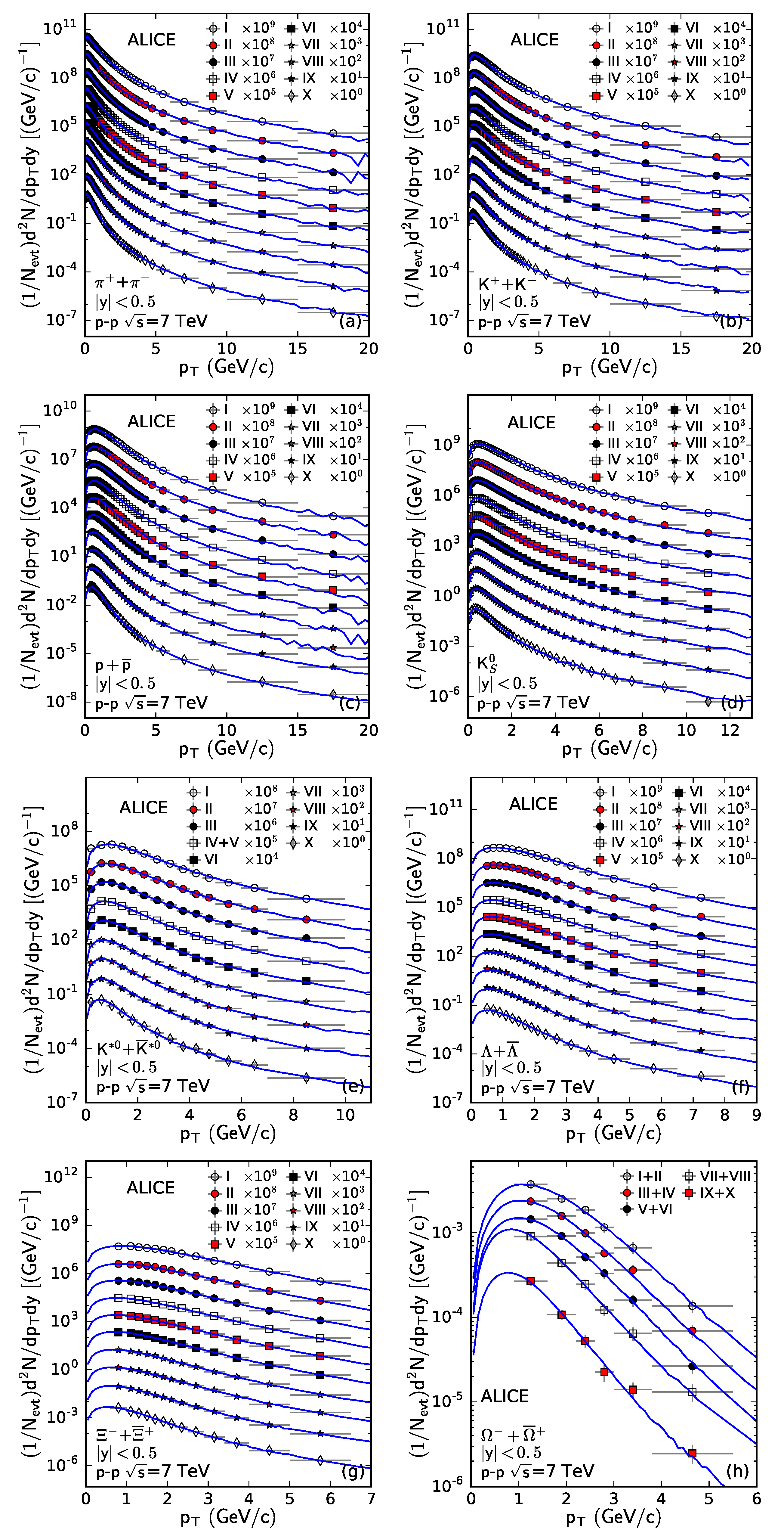
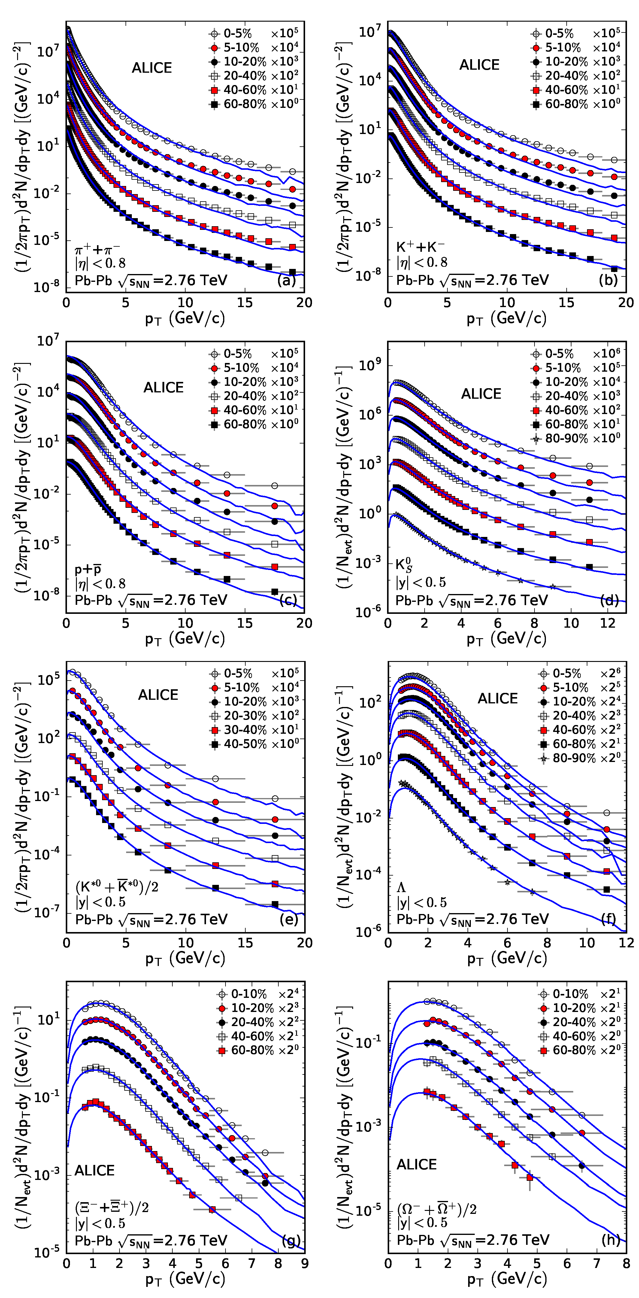
3.1. Comparison with Data

Figure 1 shows the multiplicity-dependent $p_T$ spectra and the double-differential yield $(1/N_{evt})d^{2}N/d{p}_{T}dy$ of ${\pi }^{+}+{\pi }^{-}$ (a), $K^{+}+K^{-}$ (b), $p+\overline{p}$ (c), $K_S^0$ (d), $K^{*}+\overline{K}{}^{*}$ (e), $\mathsf{\Lambda }+\overline{\mathsf{\Lambda }}$ (f), ${\mathsf{\Xi }}^{-}+\overline{\mathsf{\Xi }}{}^{+}$ (g), and ${\mathsf{\Omega }}^{-}+\overline{\mathsf{\Omega }}{}^{+}$ (h), with the rapidity $\left|y\right|<0.5$ produced in $pp$ collisions at the center-of-mass energy ($\sqrt{s}=7$ TeV), where $N_{evt}$ denotes the number of events that can be omitted in the vertical axis according to the format in the cited reference. Different symbols represent the experimental data for different multiplicity classes determined by the multiplicity measured in the VZERO detector (V0M) by the ALICE Collaboration [28], where in most of the cases the data are scaled by constant multipliers marked in the panels for clarity. The curves represent our fit results from a Monte Carlo calculation. The values of the free parameters ($a_0$, T, and n), normalization constant ($N_0$, the multiplicity in the considered rapidity region), ${\chi }^2$, and number of degrees of freedom (ndof) are listed in

Table 1. Values of the free parameters ($a_0$, T, and n), normalization constant ($N_0$), ${\chi }^2$, and number of degrees of freedom ($ndof$) corresponding to the curves in Figure 1 for $pp$ collisions at $\sqrt{s}=7$ TeV. The particle type (quark structure), spectral form, and multiplicity classes are shown together. The multiplicity classes I, II, III, IV, V, VI, VII, VIII, IX, and X correspond to the event percentile classes 0–0.95%, 0.95–4.7%, 4.7–9.5%, 9.5–14%, 14–19%, 19–28%, 28–38%, 38–48%, 48–68%, and 68–100%, respectively.

Particle (Quark Structure) and Spectrum Form	Multiplicity Class	${\mathit{a}}_0$	T (GeV)	n	${\mathit{N}}_0$	${\mathit{\chi }}^2$/ndof
	I	$-0.700\pm 0.004$	$0.320\pm 0.002$	$5.070\pm 0.054$	$(2.130\pm 0.042)\times 10$${}^1$	$58/44$
	II	$-0.700\pm 0.003$	$0.283\pm 0.003$	$4.962\pm 0.035$	$(1.700\pm 0.021)\times 10$${}^1$	$66/44$
	III	$-0.700\pm 0.004$	$0.279\pm 0.002$	$4.962\pm 0.031$	$(1.350\pm 0.040)\times {10}^1$	$69/44$
${\pi }^{+}+{\pi }^{-}$	IV	$-0.700\pm 0.004$	$0.262\pm 0.002$	$4.934\pm 0.066$	$(1.200\pm 0.030)\times {10}^1$	$66/44$
$(u\overline{d},d\overline{u})$	V	$-0.700\pm 0.005$	$0.253\pm 0.001$	$4.910\pm 0.033$	$(1.040\pm 0.101)\times {10}^1$	$65/44$
$(1/N_{evt})d^{2}N/d{p}_{T}dy$	VI	$-0.700\pm 0.005$	$0.247\pm 0.001$	$4.906\pm 0.029$	$(8.580\pm 0.080)\times$${10}^0$	$84/44$
$\left[{(\mathrm{GeV}/c)}^{-1}\right]$	VII	$-0.700\pm 0.004$	$0.236\pm 0.002$	$4.910\pm 0.086$	$(7.230\pm 0.040)\times$${10}^0$	$62/44$
	VIII	$-0.700\pm 0.003$	$0.232\pm 0.002$	$4.910\pm 0.115$	$(5.860\pm 0.030)\times {10}^0$	$69/44$
	IX	$-0.700\pm 0.003$	$0.222\pm 0.001$	$4.910\pm 0.041$	$(4.370\pm 0.101)\times {10}^0$	$104/44$
	X	$-0.700\pm 0.005$	$0.170\pm 0.002$	$4.910\pm 0.032$	$(2.750\pm 0.080)\times {10}^0$	$194/44$
	I	$-0.082\pm 0.010$	$0.253\pm 0.002$	$5.325\pm 0.028$	$(2.810\pm 0.080)\times {10}^0$	$23/39$
	II	$-0.082\pm 0.012$	$0.242\pm 0.001$	$5.321\pm 0.026$	$(2.140\pm 0.040)\times {10}^0$	$11/39$
	III	$-0.082\pm 0.024$	$0.233\pm 0.002$	$5.290\pm 0.018$	$(1.740\pm 0.020)\times {10}^0$	$7/39$
$K^{+}+K^{-}$	IV	$-0.082\pm 0.016$	$0.226\pm 0.001$	$5.245\pm 0.014$	$(1.490\pm 0.020)\times {10}^0$	$6/39$
$(u\overline{s},s\overline{u})$	V	$-0.082\pm 0.016$	$0.221\pm 0.001$	$5.260\pm 0.014$	$(1.300\pm 0.010)\times {10}^0$	$5/39$
$(1/N_{evt})d^{2}N/d{p}_{T}dy$	VI	$-0.082\pm 0.020$	$0.214\pm 0.001$	$5.253\pm 0.018$	$(1.090\pm 0.020)\times {10}^0$	$10/39$
$\left[{(\mathrm{GeV}/c)}^{-1}\right]$	VII	$-0.082\pm 0.016$	$0.207\pm 0.001$	$5.252\pm 0.023$	$(8.500\pm 0.080)\times {10}^{-1}$	$11/39$
	VIII	$-0.082\pm 0.018$	$0.197\pm 0.001$	$5.220\pm 0.025$	$(6.860\pm 0.100)\times {10}^{-1}$	$17/39$
	IX	$-0.082\pm 0.016$	$0.182\pm 0.001$	$5.214\pm 0.029$	$(5.000\pm 0.060)\times {10}^{-1}$	$22/39$
	X	$-0.082\pm 0.021$	$0.156\pm 0.002$	$5.220\pm 0.030$	$(2.900\pm 0.060)\times {10}^{-1}$	$34/39$
	I	$0.230\pm 0.008$	$0.207\pm 0.002$	$6.505\pm 0.035$	$(1.109\pm 0.009)\times {10}^0$	$5/37$
	II	$0.230\pm 0.005$	$0.199\pm 0.002$	$6.646\pm 0.075$	$(8.701\pm 0.150)\times {10}^{-1}$	$20/37$
	III	$0.230\pm 0.008$	$0.188\pm 0.001$	$6.534\pm 0.063$	$(7.079\pm 0.040)\times {10}^{-1}$	$17/37$
$p+\overline{p}$	IV	$0.230\pm 0.009$	$0.185\pm 0.001$	$6.613\pm 0.046$	$(6.130\pm 0.080)\times {10}^{-1}$	$14/37$
$(uud,\overline{u}\overline{u}\overline{d})$	V	$0.230\pm 0.008$	$0.178\pm 0.003$	$6.578\pm 0.086$	$(5.450\pm 0.090)\times {10}^{-1}$	$23/37$
$(1/N_{evt})d^{2}N/d{p}_{T}dy$	VI	$0.230\pm 0.011$	$0.167\pm 0.001$	$6.282\pm 0.080$	$(4.530\pm 0.080)\times {10}^{-1}$	$24/37$
$\left[{(\mathrm{GeV}/c)}^{-1}\right]$	VII	$0.230\pm 0.004$	$0.157\pm 0.002$	$6.313\pm 0.066$	$(3.650\pm 0.060)\times {10}^{-1}$	$16/37$
	VIII	$0.230\pm 0.009$	$0.150\pm 0.001$	$6.311\pm 0.077$	$(2.900\pm 0.050)\times {10}^{-1}$	$22/37$
	IX	$0.230\pm 0.008$	$0.138\pm 0.001$	$6.171\pm 0.076$	$(2.079\pm 0.020)\times {10}^{-1}$	$25/37$
	X	$0.230\pm 0.010$	$0.118\pm 0.001$	$6.160\pm 0.065$	$(1.120\pm 0.020)\times {10}^{-1}$	$21/37$
	I	$-0.082\pm 0.008$	$0.261\pm 0.002$	$5.722\pm 0.046$	$(1.338\pm 0.015)\times {10}^0$	$10/34$
	II	$-0.082\pm 0.007$	$0.254\pm 0.002$	$5.620\pm 0.057$	$(1.030\pm 0.010)\times {10}^0$	$35/34$
	III	$-0.082\pm 0.008$	$0.237\pm 0.001$	$5.538\pm 0.045$	$(8.360\pm 0.010)\times {10}^{-1}$	$29/34$
$K_S^0$	IV	$-0.082\pm 0.009$	$0.237\pm 0.002$	$5.625\pm 0.057$	$(7.080\pm 0.080)\times {10}^{-1}$	$35/34$
$\left(d\overline{s}\right)$	V	$-0.082\pm 0.008$	$0.230\pm 0.002$	$5.499\pm 0.057$	$(6.200\pm 0.080)\times {10}^{-1}$	$34/34$
$(1/N_{evt})d^{2}N/d{p}_{T}dy$	VI	$-0.082\pm 0.011$	$0.223\pm 0.001$	$5.405\pm 0.066$	$(5.150\pm 0.060)\times {10}^{-1}$	$46/34$
$\left[{(\mathrm{GeV}/c)}^{-1}\right]$	VII	$-0.082\pm 0.008$	$0.215\pm 0.001$	$5.518\pm 0.088$	$(4.000\pm 0.040)\times {10}^{-1}$	$70/34$
	VIII	$-0.082\pm 0.010$	$0.210\pm 0.001$	$5.480\pm 0.118$	$(3.220\pm 0.040)\times {10}^{-1}$	$70/34$
	IX	$-0.082\pm 0.007$	$0.194\pm 0.001$	$5.444\pm 0.096$	$(2.350\pm 0.030)\times {10}^{-1}$	$63/34$
	X	$-0.082\pm 0.011$	$0.163\pm 0.001$	$5.230\pm 0.057$	$(1.270\pm 0.020)\times {10}^{-1}$	$35/34$
	I	$1.150\pm 0.012$	$0.191\pm 0.001$	$7.073\pm 0.030$	$(3.250\pm 0.040)\times {10}^{-1}$	$5/10$
	II	$1.150\pm 0.006$	$0.186\pm 0.001$	$7.026\pm 0.039$	$(2.700\pm 0.029)\times {10}^{-1}$	$3/10$
$K^{*0}+\overline{K}{}^{*0}$	III	$1.150\pm 0.013$	$0.163\pm 0.002$	$6.480\pm 0.035$	$(2.300\pm 0.040)\times {10}^{-1}$	$5/10$
$(u\overline{s},s\overline{u})$	IV + V	$1.150\pm 0.018$	$0.153\pm 0.002$	$6.383\pm 0.035$	$(1.910\pm 0.030)\times {10}^{-1}$	$3/10$
$(1/N_{evt})d^{2}N/d{p}_{T}dy$	VI	$1.150\pm 0.020$	$0.141\pm 0.002$	$6.106\pm 0.086$	$(4.519\pm 0.020)\times {10}^{-1}$	$9/10$
$\left[{(\mathrm{GeV}/c)}^{-1}\right]$	VII	$1.150\pm 0.012$	$0.137\pm 0.002$	$6.265\pm 0.057$	$(1.249\pm 0.040)\times {10}^{-1}$	$9/10$
	VIII	$1.150\pm 0.016$	$0.130\pm 0.003$	$6.237\pm 0.066$	$(1.039\pm 0.020)\times {10}^{-1}$	$6/10$
	IX	$1.150\pm 0.014$	$0.118\pm 0.002$	$6.346\pm 0.106$	$(7.800\pm 0.040)\times {10}^{-2}$	$10/10$
	X	$1.150\pm 0.020$	$0.103\pm 0.002$	$6.312\pm 0.111$	$(4.800\pm 0.030)\times {10}^{-2}$	$10/10$
	I	$-0.050\pm 0.004$	$0.302\pm 0.001$	$8.651\pm 0.021$	$(7.619\pm 0.089)\times {10}^{-1}$	$12/12$
	II	$-0.050\pm 0.004$	$0.284\pm 0.001$	$8.372\pm 0.036$	$(5.900\pm 0.070)\times {10}^{-1}$	$12/12$
	III	$-0.050\pm 0.006$	$0.268\pm 0.002$	$7.907\pm 0.038$	$(4.700\pm 0.060)\times {10}^{-1}$	$10/12$
$\mathsf{\Lambda }+\overline{\mathsf{\Lambda }}$	IV	$-0.050\pm 0.015$	$0.254\pm 0.002$	$7.429\pm 0.040$	$(3.979\pm 0.060)\times {10}^{-1}$	$13/12$
$(uds,\overline{u}\overline{d}\overline{s})$	V	$-0.050\pm 0.013$	$0.241\pm 0.002$	$7.029\pm 0.042$	$(3.450\pm 0.060)\times {10}^{-1}$	$4/12$
$(1/N_{evt})d^{2}N/d{p}_{T}dy$	VI	$-0.050\pm 0.022$	$0.233\pm 0.002$	$7.025\pm 0.061$	$(2.850\pm 0.040)\times {10}^{-1}$	$12/12$
$\left[{(\mathrm{GeV}/c)}^{-1}\right]$	VII	$-0.050\pm 0.014$	$0.221\pm 0.002$	$6.968\pm 0.075$	$(2.200\pm 0.039)\times {10}^{-1}$	$7/12$
	VIII	$-0.050\pm 0.011$	$0.205\pm 0.003$	$6.738\pm 0.103$	$(1.720\pm 0.040)\times {10}^{-1}$	$12/12$
	IX	$-0.050\pm 0.012$	$0.191\pm 0.002$	$6.708\pm 0.085$	$(1.130\pm 0.030)\times {10}^{-1}$	$9/12$
	X	$-0.050\pm 0.023$	$0.165\pm 0.002$	$6.298\pm 0.129$	$(4.500\pm 0.010)\times {10}^{-2}$	$18/12$
	I	$-0.055\pm 0.004$	$0.366\pm 0.003$	$11.507\pm 0.060$	$(9.700\pm 0.069)\times {10}^{-2}$	$7/9$
	II	$-0.055\pm 0.003$	$0.345\pm 0.001$	$10.215\pm 0.043$	$(7.000\pm 0.060)\times {10}^{-2}$	$14/9$
	III	$-0.055\pm 0.006$	$0.307\pm 0.001$	$8.700\pm 0.026$	$(6.000\pm 0.060)\times {10}^{-2}$	$4/9$
${\mathsf{\Xi }}^{-}+\overline{\mathsf{\Xi }}{}^{+}$	IV	$-0.055\pm 0.005$	$0.301\pm 0.001$	$8.553\pm 0.034$	$(4.800\pm 0.019)\times {10}^{-2}$	$5/9$
$(ssd,\overline{s}\overline{s}\overline{d})$	V	$-0.055\pm 0.005$	$0.283\pm 0.001$	$7.629\pm 0.027$	$(3.999\pm 0.010)\times {10}^{-2}$	$4/9$
$(1/N_{evt})d^{2}N/d{p}_{T}dy$	VI	$-0.055\pm 0.010$	$0.270\pm 0.001$	$7.466\pm 0.035$	$(3.400\pm 0.020)\times {10}^{-2}$	$3/9$
$\left[{(\mathrm{GeV}/c)}^{-1}\right]$	VII	$-0.055\pm 0.005$	$0.258\pm 0.001$	$7.376\pm 0.031$	$(2.579\pm 0.025)\times {10}^{-2}$	$4/9$
	VIII	$-0.055\pm 0.007$	$0.242\pm 0.001$	$6.844\pm 0.035$	$(1.899\pm 0.010)\times {10}^{-2}$	$6/9$
	IX	$-0.055\pm 0.006$	$0.214\pm 0.001$	$6.255\pm 0.018$	$(1.240\pm 0.012)\times {10}^{-2}$	$2/9$
	X	$-0.055\pm 0.009$	$0.189\pm 0.001$	$6.090\pm 0.033$	$(5.399\pm 0.199)\times {10}^{-3}$	$4/9$
${\mathsf{\Omega }}^{-}+\overline{\mathsf{\Omega }}{}^{+}$	I + II	$0.360\pm 0.004$	$0.312\pm 0.002$	$9.597\pm 0.031$	$(8.099\pm 0.010)\times {10}^{-3}$	$1/2$
$(sss,\overline{s}\overline{s}\overline{s})$	III + IV	$0.360\pm 0.004$	$0.294\pm 0.002$	$9.548\pm 0.033$	$(4.899\pm 0.010)\times {10}^{-3}$	$2/2$
$(1/N_{evt})d^{2}N/d{p}_{T}dy$	V + VI	$0.360\pm 0.005$	$0.270\pm 0.002$	$9.572\pm 0.032$	$(2.899\pm 0.010)\times {10}^{-3}$	$1/2$
$\left[{(\mathrm{GeV}/c)}^{-1}\right]$	VII + VIII	$0.360\pm 0.004$	$0.215\pm 0.002$	$6.477\pm 0.030$	$(1.820\pm 0.009)\times {10}^{-3}$	$1/2$
	IX + X	$0.360\pm 0.004$	$0.192\pm 0.002$	$6.477\pm 0.031$	$(5.200\pm 0.001)\times {10}^{-4}$	$3/2$

, in which the particle type, the quark structure that makes up the hadrons, and the form of the spectra are all mentioned. The corresponding serial numbers of the V0M classes marked with Roman numerals in the figure are listed in Table 1 in terms of the percentage of classes that can be regarded as the event percentile classes. It can be seen that our fit results are in good agreement with the experimental data measured by the ALICE Collaboration at midrapidity in $pp$ collisions at $\sqrt{s}=7$ TeV.

Similar to Figure 1, Figure 2 shows the multiplicity-dependent $p_T$ spectra and the double-differential yield $(1/N_{evt})d^{2}N/d{p}_{T}dy$ of ${\pi }^{+}+{\pi }^{-}$ (a), $K^{+}+K^{-}$ (b), $p+\overline{p}$ (c), $K_S^0$ (d), $K^{*0}$ (e), $\mathsf{\Lambda }+\overline{\mathsf{\Lambda }}$ (f), ${\mathsf{\Xi }}^{-}+\overline{\mathsf{\Xi }}{}^{+}$ (g), and ${\mathsf{\Omega }}^{-}+\overline{\mathsf{\Omega }}{}^{+}$ (h), with $\left|y\right|<0.5$ (produced in $pp$ collisions at $\sqrt{s}=13$ TeV) measured by the ALICE Collaboration [51,52,53]. Different symbols represent the data for different serial numbers of V0M classes, marked by the Roman numerals, and the corresponding event percentile classes listed in

Table 2. Values of $a_0$, T, n, $N_0$, ${\chi }^2$, and $ndof$ corresponding to the curves in Figure 2 for $pp$ collisions at $\sqrt{s}=13$ TeV. The particle type (quark structure), spectrum form, and multiplicity classes are shown together. The multiplicity classes I, II, III, IV, V, VI, VII, VIII, IX, and X for ${\pi }^{+}+{\pi }^{-}$, $K^{+}+K^{-}$, and $p+\overline{p}$ correspond to the event percentile classes 0–0.92%, 0.92–4.6%, 4.6–9.2%, 9.2–13.8%, 13.8–18.4%, 18.4–27.6%, 27.6–36.8%, 36.8–46%, 46–64.5%, and 64.5–100%, respectively, and $K_S^0$, $K^{*0}$, $\mathsf{\Lambda }+\overline{\mathsf{\Lambda }}$, ${\mathsf{\Xi }}^{-}+\overline{\mathsf{\Xi }}{}^{+}$, and ${\mathsf{\Omega }}^{-}+\overline{\mathsf{\Omega }}{}^{+}$ correspond to the event percentile classes 0–0.9%, 0.9–4.5%, 4.5–8.9%, 8.9–13.5%, 13.5–18%, 18–27%, 27–36.1%, 36.1–45.3%, 45.3–64.5%, and 64.5–100%, respectively.

Particle (Quark Structure) and Spectrum Form	Multiplicity Class	${\mathit{a}}_0$	T (GeV)	n	${\mathit{N}}_0$	${\mathit{\chi }}^2$/ndof
	I	$-0.750\pm 0.003$	$0.328\pm 0.002$	$4.996\pm 0.045$	$(2.599\pm 0.070)\times 10$${}^1$	$56/47$
	II	$-0.750\pm 0.002$	$0.320\pm 0.002$	$4.945\pm 0.022$	$(2.030\pm 0.030)\times {10}^1$	$74/47$
	III	$-0.750\pm 0.004$	$0.308\pm 0.004$	$4.870\pm 0.021$	$(1.670\pm 0.020)\times {10}^1$	$70/47$
${\pi }^{+}+{\pi }^{-}$	IV	$-0.750\pm 0.005$	$0.300\pm 0.002$	$4.874\pm 0.026$	$(1.400\pm 0.019)\times {10}^1$	$60/47$
$(u\overline{d},d\overline{u})$	V	$-0.750\pm 0.005$	$0.285\pm 0.002$	$4.874\pm 0.035$	$(1.250\pm 0.002)\times {10}^1$	$55/47$
$(1/N_{evt})d^{2}N/d{p}_{T}dy$	VI	$-0.750\pm 0.005$	$0.270\pm 0.001$	$7.366\pm 0.020$	$(1.030\pm 0.014)\times {10}^1$	$44/47$
$\left[{(\mathrm{GeV}/c)}^{-1}\right]$	VII	$-0.750\pm 0.002$	$0.270\pm 0.001$	$4.870\pm 0.016$	$(8.229\pm 0.089)\times 10$${}^0$	$49/47$
	VIII	$-0.750\pm 0.004$	$0.266\pm 0.001$	$4.870\pm 0.029$	$(6.730\pm 0.070)\times {10}^0$	$56/47$
	IX	$-0.750\pm 0.004$	$0.249\pm 0.001$	$4.865\pm 0.028$	$(4.840\pm 0.050)\times {10}^0$	$92/47$
	X	$-0.750\pm 0.005$	$0.203\pm 0.002$	$4.861\pm 0.022$	$(2.800\pm 0.050)\times {10}^0$	$324/47$
	I	$-0.082\pm 0.003$	$0.267\pm 0.003$	$5.186\pm 0.082$	$(3.179\pm 0.040)\times {10}^0$	$15/42$
	II	$-0.082\pm 0.002$	$0.260\pm 0.002$	$5.273\pm 0.021$	$(2.580\pm 0.040)\times {10}^0$	$9/42$
	III	$-0.082\pm 0.003$	$0.252\pm 0.001$	$5.243\pm 0.018$	$(2.060\pm 0.030)\times {10}^0$	$14/42$
$K^{+}+K^{-}$	IV	$-0.082\pm 0.005$	$0.244\pm 0.002$	$5.150\pm 0.021$	$(1.740\pm 0.019)\times {10}^0$	$25/42$
$(u\overline{s},s\overline{u})$	V	$-0.082\pm 0.005$	$0.237\pm 0.001$	$5.130\pm 0.022$	$(1.540\pm 0.020)\times {10}^0$	$24/42$
$(1/N_{evt})d^{2}N/d{p}_{T}dy$	VI	$-0.082\pm 0.005$	$0.233\pm 0.003$	$5.242\pm 0.022$	$(1.250\pm 0.019)\times {10}^0$	$43/42$
$\left[{(\mathrm{GeV}/c)}^{-1}\right]$	VII	$-0.082\pm 0.004$	$0.224\pm 0.001$	$5.217\pm 0.023$	$(9.799\pm 0.100)\times {10}^{-1}$	$47/42$
	VIII	$-0.082\pm 0.003$	$0.213\pm 0.002$	$5.223\pm 0.025$	$(7.700\pm 0.080)\times {10}^{-1}$	$54/42$
	IX	$-0.082\pm 0.003$	$0.196\pm 0.002$	$5.174\pm 0.027$	$(5.370\pm 0.070)\times {10}^{-1}$	$67/42$
	X	$-0.082\pm 0.005$	$0.165\pm 0.002$	$5.138\pm 0.024$	$(2.970\pm 0.040)\times {10}^{-1}$	$464/41$
	I	$0.230\pm 0.011$	$0.222\pm 0.002$	$6.291\pm 0.012$	$(1.379\pm 0.029)\times {10}^0$	$31/40$
	II	$0.230\pm 0.013$	$0.208\pm 0.002$	$6.278\pm 0.096$	$(1.060\pm 0.020)\times {10}^0$	$24/40$
	III	$0.230\pm 0.012$	$0.197\pm 0.002$	$6.267\pm 0.044$	$(8.799\pm 0.149)\times {10}^{-1}$	$22/40$
$p+\overline{p}$	IV	$0.230\pm 0.011$	$0.190\pm 0.001$	$6.278\pm 0.012$	$(7.299\pm 0.090)\times {10}^{-1}$	$26/40$
$(uud,\overline{u}\overline{u}\overline{d})$	V	$0.230\pm 0.013$	$0.184\pm 0.003$	$6.242\pm 0.033$	$(6.499\pm 0.079)\times {10}^{-1}$	$20/40$
$(1/N_{evt})d^{2}N/d{p}_{T}dy$	VI	$0.230\pm 0.023$	$0.175\pm 0.001$	$6.216\pm 0.055$	$(5.600\pm 0.080)\times {10}^{-1}$	$27/40$
$\left[{(\mathrm{GeV}/c)}^{-1}\right]$	VII	$0.230\pm 0.022$	$0.165\pm 0.002$	$6.100\pm 0.031$	$(4.300\pm 0.050)\times {10}^{-1}$	$31/40$
	VIII	$0.230\pm 0.015$	$0.157\pm 0.002$	$6.100\pm 0.033$	$(3.450\pm 0.060)\times {10}^{-1}$	$40/40$
	IX	$0.230\pm 0.009$	$0.145\pm 0.001$	$6.100\pm 0.036$	$(2.360\pm 0.040)\times {10}^{-1}$	$48/40$
	X	$0.230\pm 0.005$	$0.117\pm 0.001$	$5.804\pm 0.028$	$(1.249\pm 0.029)\times {10}^{-1}$	$36/40$
	I	$0.048\pm 0.003$	$0.261\pm 0.002$	$5.357\pm 0.033$	$(1.610\pm 0.019)\times {10}^0$	$18/34$
	II	$0.048\pm 0.005$	$0.243\pm 0.002$	$5.384\pm 0.038$	$(1.210\pm 0.080)\times {10}^0$	$33/34$
	III	$0.048\pm 0.004$	$0.233\pm 0.002$	$5.401\pm 0.063$	$(9.899\pm 0.079)\times {10}^{-1}$	$37/34$
$K_S^0$	IV	$0.048\pm 0.003$	$0.223\pm 0.001$	$5.270\pm 0.032$	$(8.500\pm 0.040)\times {10}^{-1}$	$27/34$
$\left(d\overline{s}\right)$	V	$0.048\pm 0.005$	$0.219\pm 0.002$	$5.262\pm 0.024$	$(7.500\pm 0.080)\times {10}^{-1}$	$35/34$
$(1/N_{evt})d^{2}N/d{p}_{T}dy$	VI	$0.048\pm 0.003$	$0.213\pm 0.001$	$5.260\pm 0.036$	$(6.239\pm 0.069)\times {10}^{-1}$	$54/34$
$\left[{(\mathrm{GeV}/c)}^{-1}\right]$	VII	$0.048\pm 0.004$	$0.207\pm 0.002$	$5.259\pm 0.048$	$(4.850\pm 0.040)\times {10}^{-1}$	$65/34$
	VIII	$0.048\pm 0.004$	$0.193\pm 0.001$	$5.232\pm 0.043$	$(3.930\pm 0.050)\times {10}^{-1}$	$64/34$
	IX	$0.048\pm 0.003$	$0.183\pm 0.001$	$5.229\pm 0.008$	$(2.760\pm 0.030)\times {10}^{-1}$	$60/34$
	X	$0.048\pm 0.003$	$0.163\pm 0.001$	$5.222\pm 0.037$	$(1.440\pm 0.029)\times {10}^{-1}$	$51/34$
	I	$1.150\pm 0.022$	$0.209\pm 0.002$	$6.978\pm 0.013$	$(4.569\pm 0.150)\times {10}^{-1}$	$2/8$
	II	$1.150\pm 0.028$	$0.196\pm 0.002$	$6.925\pm 0.008$	$(3.619\pm 0.080)\times {10}^{-1}$	$8/10$
$K^{*0}$	III	$1.150\pm 0.035$	$0.190\pm 0.003$	$6.805\pm 0.013$	$(2.899\pm 0.070)\times {10}^{-1}$	$8/10$
$\left(d\overline{s}\right)$	IV + V	$1.150\pm 0.030$	$0.168\pm 0.002$	$6.288\pm 0.016$	$(2.379\pm 0.010)\times {10}^{-1}$	$16/10$
$(1/N_{evt})d^{2}N/d{p}_{T}dy$	VI	$1.150\pm 0.028$	$0.168\pm 0.004$	$6.587\pm 0.006$	$(1.829\pm 0.089)\times {10}^{-1}$	$12/10$
$\left[{(\mathrm{GeV}/c)}^{-1}\right]$	VII	$1.150\pm 0.018$	$0.159\pm 0.005$	$6.410\pm 0.008$	$(1.519\pm 0.040)\times {10}^{-1}$	$18/10$
	VIII	$1.150\pm 0.025$	$0.146\pm 0.003$	$6.415\pm 0.013$	$(1.219\pm 0.050)\times {10}^{-1}$	$17/10$
	IX	$1.150\pm 0.026$	$0.132\pm 0.002$	$6.104\pm 0.008$	$(8.600\pm 0.026)\times {10}^{-2}$	$17/10$
	X	$1.150\pm 0.018$	$0.108\pm 0.003$	$6.018\pm 0.007$	$(4.700\pm 0.029)\times {10}^{-2}$	$24/10$
	I	$-0.023\pm 0.021$	$0.327\pm 0.003$	$8.885\pm 0.013$	$(9.499\pm 0.130)\times {10}^{-1}$	$11/12$
	II	$-0.023\pm 0.012$	$0.298\pm 0.004$	$8.328\pm 0.112$	$(7.419\pm 0.180)\times {10}^{-1}$	$15/12$
	III	$-0.023\pm 0.014$	$0.292\pm 0.002$	$8.328\pm 0.091$	$(5.999\pm 0.100)\times {10}^{-1}$	$7/12$
$\mathsf{\Lambda }+\overline{\mathsf{\Lambda }}$	IV	$-0.023\pm 0.008$	$0.293\pm 0.003$	$7.402\pm 0.093$	$(5.099\pm 0.150)\times {10}^{-1}$	$7/12$
$(uds,\overline{u}\overline{d}\overline{s})$	V	$-0.023\pm 0.011$	$0.292\pm 0.002$	$7.355\pm 0.043$	$(4.500\pm 0.050)\times {10}^{-1}$	$5/12$
$(1/N_{evt})d^{2}N/d{p}_{T}dy$	VI	$-0.023\pm 0.022$	$0.283\pm 0.001$	$7.351\pm 0.052$	$(3.669\pm 0.080)\times {10}^{-1}$	$10/12$
$\left[{(\mathrm{GeV}/c)}^{-1}\right]$	VII	$-0.023\pm 0.019$	$0.259\pm 0.002$	$6.553\pm 0.063$	$(3.060\pm 0.049)\times {10}^{-1}$	$8/12$
	VIII	$-0.023\pm 0.014$	$0.243\pm 0.003$	$6.554\pm 0.081$	$(2.339\pm 0.040)\times {10}^{-1}$	$7/12$
	IX	$-0.023\pm 0.012$	$0.225\pm 0.001$	$6.456\pm 0.043$	$(1.560\pm 0.040)\times {10}^{-1}$	$10/12$
	X	$-0.023\pm 0.025$	$0.189\pm 0.001$	$6.200\pm 0.019$	$(6.899\pm 0.026)\times {10}^{-2}$	$15/12$
	I	$-0.150\pm 0.008$	$0.417\pm 0.002$	$11.059\pm 0.048$	$(1.299\pm 0.013)\times {10}^{-1}$	$7/9$
	II	$-0.150\pm 0.007$	$0.390\pm 0.003$	$10.013\pm 0.093$	$(9.600\pm 0.140)\times {10}^{-2}$	$9/9$
	III	$-0.150\pm 0.013$	$0.372\pm 0.003$	$9.603\pm 0.190$	$(7.599\pm 0.219)\times {10}^{-2}$	$16/9$
${\mathsf{\Xi }}^{-}+\overline{\mathsf{\Xi }}{}^{+}$	IV	$-0.150\pm 0.011$	$0.358\pm 0.002$	$9.590\pm 0.112$	$(6.099\pm 0.120)\times {10}^{-2}$	$9/9$
$(ssd,\overline{s}\overline{s}\overline{d})$	V	$-0.150\pm 0.021$	$0.353\pm 0.003$	$9.558\pm 0.170$	$(5.399\pm 0.140)\times {10}^{-2}$	$16/9$
$(1/N_{evt})d^{2}N/d{p}_{T}dy$	VI	$-0.150\pm 0.012$	$0.321\pm 0.002$	$9.527\pm 0.087$	$(4.299\pm 0.130)\times {10}^{-2}$	$22/9$
$\left[{(\mathrm{GeV}/c)}^{-1}\right]$	VII	$-0.150\pm 0.013$	$0.315\pm 0.002$	$8.985\pm 0.152$	$(3.199\pm 0.080)\times {10}^{-2}$	$10/9$
	VIII	$-0.150\pm 0.007$	$0.280\pm 0.002$	$8.000\pm 0.122$	$(2.600\pm 0.070)\times {10}^{-2}$	$13/9$
	IX	$-0.150\pm 0.004$	$0.246\pm 0.001$	$6.353\pm 0.088$	$(1.600\pm 0.010)\times {10}^{-2}$	$6/9$
	X	$-0.150\pm 0.012$	$0.215\pm 0.002$	$6.523\pm 0.080$	$(5.900\pm 0.160)\times {10}^{-3}$	$5/9$
${\mathsf{\Omega }}^{-}+\overline{\mathsf{\Omega }}{}^{+}$	I + II	$0.360\pm 0.021$	$0.336\pm 0.001$	$9.624\pm 0.013$	$(1.020\pm 0.003)\times {10}^{-2}$	$-/2$
$(sss,\overline{s}\overline{s}\overline{s})$	III + IV	$0.360\pm 0.018$	$0.290\pm 0.001$	$9.632\pm 0.013$	$(4.100\pm 0.200)\times {10}^{-3}$	$5/2$
$(1/N_{evt})d^{2}N/d{p}_{T}dy$	V + VI	$0.360\pm 0.020$	$0.288\pm 0.001$	$9.612\pm 0.016$	$(4.099\pm 0.150)\times {10}^{-3}$	$4/2$
$\left[{(\mathrm{GeV}/c)}^{-1}\right]$	VII + VIII	$0.360\pm 0.004$	$0.276\pm 0.002$	$9.640\pm 0.008$	$(1.900\pm 0.080)\times {10}^{-3}$	$8/2$
	IX + X	$0.360\pm 0.022$	$0.241\pm 0.003$	$9.622\pm 0.008$	$(6.299\pm 0.150)\times {10}^{-4}$	$1/1$

. The curves show our results from the Monte Carlo calculation used to fit the data. Certain data were scaled by multiplication by the different numbers marked in the panels for clarity. The values of $a_0$, T, n, N, ${\chi }^2/ndof$, and other related information are provided in Table 2. From the figure and ${\chi }^2/ndof$, it can be seen that our fit results are in good agreement with the experimental data measured by the ALICE Collaboration at midrapidity in $pp$ collisions at $\sqrt{s}=13$ TeV.

Similar to Figure 1 and Figure 2, Figure 3 displays the centrality-dependent $p_T$ spectra, the invariant yield $(1/2\pi p_T)d^{2}N/d{p}_{T}dy$ (a–c) or $(1/N_{evt}2\pi p_T)d^{2}N/d{p}_{T}dy$ (d, f–h) or the double-differential yield $(1/N_{evt})d^{2}N/d{p}_{T}dy$ (e) of ${\pi }^{+}+{\pi }^{-}$ (a), $K^{+}+K^{-}$ (b), $p+\overline{p}$ (c), $K_S^0$ (d), $\sum {\left(1385\right)}^{+}$ (e), $\mathsf{\Lambda }+\overline{\mathsf{\Lambda }}$ (f), $({\mathsf{\Xi }}^{-}+\overline{\mathsf{\Xi }}{}^{+})/2$ (g), and $({\mathsf{\Omega }}^{-}+\overline{\mathsf{\Omega }}{}^{+})/2$ (h), with $-0.5<y<0$ (a–c, e, g, h) or $0<y<0.5$ (d, f) produced in p–Pb collisions at $\sqrt{s_{NN}}=5.02$ TeV measured by the ALICE Collaboration [10,11,54,55]. Different symbols represent those experimental data with different centrality classes, with different constant multipliers used to re-scale the data for clarity. The curves are our fit results based on a Monte Carlo calculation. The values of $a_0$, T, n, $N_0$, and ${\chi }^2/ndof$ are listed in

Table 3. Values of $a_0$, T, n, $N_0$, ${\chi }^2$, and $ndof$ corresponding to the curves in Figure 3 for p–Pb collisions at $\sqrt{s_{NN}}=5.02$ TeV. The particle type (quark structure), spectrum form, and centrality are shown together.

Particle (Quark Structure) Spectrum Form	Centrality	${\mathit{a}}_0$	T (GeV)	n	${\mathit{N}}_0$	${\mathit{\chi }}^2$/ndof
	0–5%	$-0.750\pm 0.003$	$0.346\pm 0.003$	$6.234\pm 0.063$	$(2.130\pm 0.025)\times 10$${}^1$	$148/54$
${\pi }^{+}+{\pi }^{-}$	5–10%	$-0.750\pm 0.004$	$0.343\pm 0.002$	$6.010\pm 0.072$	$(1.743\pm 0.028)\times {10}^1$	$135/54$
$(u\overline{d},d\overline{u})$	10–20%	$-0.750\pm 0.004$	$0.319\pm 0.001$	$5.630\pm 0.121$	$(1.461\pm 0.025)\times {10}^1$	$148/54$
$(1/N_{evt}2\pi p_T)d^{2}N/d{p}_{T}dy$	20–40%	$-0.750\pm 0.005$	$0.327\pm 0.001$	$5.618\pm 0.030$	$(1.153\pm 0.019)\times {10}^1$	$142/54$
$\left[{(\mathrm{GeV}/c)}^{-2}\right]$	40–60%	$-0.750\pm 0.004$	$0.295\pm 0.002$	$5.335\pm 0.034$	$(8.168\pm 0.251)\times 10$${}^0$	$130/54$
	60–80%	$-0.750\pm 0.002$	$0.293\pm 0.002$	$5.332\pm 0.033$	$(5.027\pm 0.094)\times {10}^0$	$93/54$
	80–100%	$-0.750\pm 0.003$	$0.250\pm 0.001$	$5.078\pm 0.038$	$(2.199\pm 0.072)\times {10}^0$	$173/54$
	0–5%	$-0.060\pm 0.007$	$0.265\pm 0.002$	$5.968\pm 0.021$	$(2.859\pm 0.060)\times {10}^0$	$98/47$
$K^{+}+K^{-}$	5–10%	$-0.060\pm 0.013$	$0.260\pm 0.004$	$5.948\pm 0.083$	$(2.356\pm 0.063)\times {10}^0$	$53/47$
$(u\overline{s},s\overline{u})$	10–20%	$-0.060\pm 0.006$	$0.254\pm 0.002$	$5.872\pm 0.061$	$(1.948\pm 0.038)\times {10}^0$	$36/47$
$(1/N_{evt}2\pi p_T)d^{2}N/d{p}_{T}dy$	20–40%	$-0.060\pm 0.006$	$0.253\pm 0.002$	$5.878\pm 0.046$	$(1.445\pm 0.025)\times {10}^0$	$42/47$
$\left[{(\mathrm{GeV}/c)}^{-2}\right]$	40–60%	$-0.060\pm 0.003$	$0.241\pm 0.001$	$5.741\pm 0.053$	$(9.927\pm 0.031)\times {10}^{-1}$	$54/47$
	60–80%	$-0.060\pm 0.006$	$0.216\pm 0.003$	$5.446\pm 0.048$	$(6.283\pm 0.157)\times {10}^{-1}$	$37/47$
	80–100%	$-0.060\pm 0.007$	$0.190\pm 0.002$	$5.444\pm 0.056$	$(2.419\pm 0.062)\times {10}^{-1}$	$88/47$
	0–5%	$-0.040\pm 0.021$	$0.283\pm 0.003$	$8.270\pm 0.063$	$(2.262\pm 0.075)\times {10}^0$	$89/45$
$p+\overline{p}$	5–10%	$-0.040\pm 0.012$	$0.274\pm 0.002$	$8.155\pm 0.120$	$(1.847\pm 0.062)\times {10}^0$	$41/45$
$(uud,\overline{u}\overline{u}\overline{d})$	10–20%	$-0.040\pm 0.024$	$0.267\pm 0.004$	$7.900\pm 0.111$	$(1.558\pm 0.037)\times {10}^0$	$48/45$
$(1/N_{evt}2\pi p_T)d^{2}N/d{p}_{T}dy$	20–40%	$-0.040\pm 0.021$	$0.256\pm 0.004$	$7.885\pm 0.112$	$(1.225\pm 0.019)\times {10}^0$	$29/45$
$\left[{(\mathrm{GeV}/c)}^{-2}\right]$	40–60%	$-0.040\pm 0.024$	$0.240\pm 0.004$	$7.632\pm 0.052$	$(8.357\pm 0.125)\times {10}^{-1}$	$57/45$
	60–80%	$-0.040\pm 0.029$	$0.215\pm 0.003$	$7.145\pm 0.066$	$(5.341\pm 0.144)\times {10}^{-1}$	$50/45$
	0–5%	$0.100\pm 0.005$	$0.240\pm 0.002$	$6.451\pm 0.052$	$(1.445\pm 0.028)\times {10}^0$	$16/30$
$K_S^0$	5–10%	$0.100\pm 0.007$	$0.238\pm 0.003$	$6.436\pm 0.068$	$(1.162\pm 0.028)\times {10}^0$	$20/30$
$\left(d\overline{s}\right)$	10–20%	$0.100\pm 0.010$	$0.237\pm 0.002$	$6.426\pm 0.049$	$(9.581\pm 0.157)\times {10}^{-1}$	$43/30$
$(1/N_{evt}2\pi p_T)d^{2}N/d{p}_{T}dy$	20–40%	$0.100\pm 0.008$	$0.222\pm 0.002$	$5.859\pm 0.062$	$(7.383\pm 0.219)\times {10}^{-1}$	$21/30$
$\left[{(\mathrm{GeV}/c)}^{-2}\right]$	40–60%	$0.100\pm 0.010$	$0.215\pm 0.002$	$5.762\pm 0.061$	$(5.027\pm 0.126)\times {10}^{-1}$	$35/30$
	60–80%	$0.100\pm 0.013$	$0.195\pm 0.001$	$5.487\pm 0.058$	$(3.079\pm 0.072)\times {10}^{-1}$	$38/30$
	80–100%	$0.100\pm 0.011$	$0.167\pm 0.002$	$5.025\pm 0.059$	$(1.319\pm 0.053)\times {10}^{-1}$	$59/30$
$\sum {\left(1385\right)}^{+}$$\left(suu\right)$	0–20%	$0.945\pm 0.006$	$0.201\pm 0.002$	$7.682\pm 0.065$	$(4.441\pm 0.050)\times {10}^{-2}$	$2/2$
$(1/N_{evt}2\pi p_T)d^{2}N/d{p}_{T}dy$	20–60%	$0.945\pm 0.004$	$0.183\pm 0.001$	$7.661\pm 0.056$	$(2.396\pm 0.035)\times {10}^{-2}$	$5/2$
$\left[{(\mathrm{GeV}/c)}^{-2}\right]$	60–100%	$0.945\pm 0.008$	$0.157\pm 0.002$	$7.523\pm 0.077$	$(6.596\pm 0.035)\times {10}^{-3}$	$10/2$
	0–5%	$1.000\pm 0.010$	$0.181\pm 0.001$	$8.512\pm 0.058$	$(8.167\pm 0.220)\times {10}^{-1}$	$6/16$
$\mathsf{\Lambda }+\overline{\mathsf{\Lambda }}$	5–10%	$1.000\pm 0.010$	$0.177\pm 0.001$	$8.187\pm 0.055$	$(6.439\pm 0.094)\times {10}^{-1}$	$7/16$
$(uds,\overline{u}\overline{d}\overline{s})$	10–20%	$1.000\pm 0.011$	$0.174\pm 0.003$	$8.187\pm 0.063$	$(5.403\pm 0.063)\times {10}^{-1}$	$8/16$
$(1/N_{evt}2\pi p_T)d^{2}N/d{p}_{T}dy$	20–40%	$1.000\pm 0.005$	$0.165\pm 0.001$	$7.731\pm 0.052$	$(4.083\pm 0.037)\times {10}^{-1}$	$12/16$
$\left[{(\mathrm{GeV}/c)}^{-2}\right]$	40–60%	$1.000\pm 0.018$	$0.152\pm 0.003$	$7.611\pm 0.089$	$(2.764\pm 0.069)\times {10}^{-1}$	$15/16$
	60–80%	$1.000\pm 0.023$	$0.131\pm 0.002$	$6.958\pm 0.083$	$(1.633\pm 0.041)\times {10}^{-1}$	$16/16$
	80–100%	$1.000\pm 0.019$	$0.114\pm 0.002$	$6.622\pm 0.102$	$(6.283\pm 0.251)\times {10}^{-2}$	$17/16$
	0–5%	$0.620\pm 0.031$	$0.253\pm 0.003$	$9.399\pm 0.102$	$(5.781\pm 0.079)\times {10}^{-2}$	$13/13$
$({\mathsf{\Xi }}^{-}+{\overline{\mathsf{\Xi }}}^{+})/2$	5–10%	$0.620\pm 0.019$	$0.247\pm 0.004$	$8.964\pm 0.103$	$(4.618\pm 0.110)\times {10}^{-2}$	$12/13$
$(ssd,\overline{s}\overline{s}\overline{d})$	10–20%	$0.620\pm 0.018$	$0.241\pm 0.003$	$8.882\pm 0.089$	$(3.770\pm 0.085)\times {10}^{-2}$	$10/13$
$(1/N_{evt}2\pi p_T)d^{2}N/d{p}_{T}dy$	20–40%	$0.620\pm 0.007$	$0.235\pm 0.001$	$8.824\pm 0.086$	$(2.733\pm 0.050)\times {10}^{-2}$	$15/13$
$\left[{(\mathrm{GeV}/c)}^{-2}\right]$	40–60%	$0.620\pm 0.023$	$0.222\pm 0.002$	$8.919\pm 0.079$	$(1.791\pm 0.053)\times {10}^{-2}$	$11/13$
	60–80%	$0.620\pm 0.002$	$0.203\pm 0.001$	$8.000\pm 0.001$	$(10.052\pm 0.003)\times {10}^{-3}$	$22/12$
	80–100%	$0.620\pm 0.000$	$0.160\pm 0.000$	$6.304\pm 0.001$	$(3.383\pm 0.003)\times {10}^{-3}$	$41/11$
	0–5%	$0.500\pm 0.008$	$0.319\pm 0.002$	$8.746\pm 0.062$	$(6.597\pm 0.087)\times {10}^{-3}$	$11/4$
$({\mathsf{\Omega }}^{-}+\overline{\mathsf{\Omega }}{}^{+})/2$	5–10%	$0.500\pm 0.006$	$0.319\pm 0.002$	$8.139\pm 0.088$	$(5.655\pm 0.094)\times {10}^{-3}$	$8/4$
$(sss,\overline{s}\overline{s}\overline{s})$	10–20%	$0.500\pm 0.021$	$0.294\pm 0.004$	$7.722\pm 0.103$	$(4.398\pm 0.069)\times {10}^{-3}$	$10/4$
$(1/N_{evt}2\pi p_T)d^{2}N/d{p}_{T}dy$	20–40%	$0.500\pm 0.021$	$0.278\pm 0.002$	$7.233\pm 0.111$	$(3.047\pm 0.038)\times {10}^{-3}$	$2/4$
$\left[{(\mathrm{GeV}/c)}^{-2}\right]$	40–60%	$0.500\pm 0.008$	$0.243\pm 0.003$	$6.832\pm 0.193$	$(1.885\pm 0.063)\times {10}^{-3}$	$7/4$
	60–80%	$0.500\pm 0.011$	$0.234\pm 0.002$	$6.901\pm 0.098$	$(1.005\pm 0.019)\times {10}^{-2}$	$5/4$
	80–100%	$0.500\pm 0.018$	$0.182\pm 0.003$	$6.003\pm 0.105$	$(2.984\pm 0.016)\times {10}^{-4}$	$2/4$

along with other information. It can be seen that our fit results are in agreement with the experimental data measured by the ALICE Collaboration at mid-y in p–Pb collisions at $\sqrt{s_{NN}}=5.02$ TeV.

Similar to Figure 1, Figure 2 and Figure 3, Figure 4 shows the centrality-dependent $p_T$ spectra and the invariant yield $(1/2\pi p_T)d^{2}N/d{p}_{T}dy$ (a–c, e) or double-differential yield $(1/N_{evt})d^{2}N/d{p}_{T}dy$ (d, f–h) of ${\pi }^{+}+{\pi }^{-}$ (a), $K^{+}+K^{-}$ (b), $p+\overline{p}$ (c), $K_S^0$ (d), $(K^{*0}+\overline{K}{}^{*0})/2$ (e), $\mathsf{\Lambda }$ (f), $({\mathsf{\Xi }}^{-}+\overline{\mathsf{\Xi }}{}^{+})/2$ (g), and $({\mathsf{\Omega }}^{-}+\overline{\mathsf{\Omega }}{}^{+})/2$ (h) with $\left|\eta \right|<0.8$ (a–c) or $\left|y\right|<0.5$ (d–h) produced in Pb–Pb collisions at $\sqrt{s_{NN}}=2.76$ TeV measured by the ALICE Collaboration [56,57,58,59]. The symbols represent the experimental data and the curves are our fit results. The values of $a_0$, T, n, $N_0$, and ${\chi }^2/ndof$ are listed in

Table 4. Values of $a^0$, T, n, $N_0$, ${\chi }^2$, and $ndof$ corresponding to the curves in Figure 4 for Pb–Pb collisions at $\sqrt{s_{NN}}=2.76$ TeV. The particle type (quark structure), spectrum form, and centrality are shown together.

Particle (Quark Structure) Spectrum Form	Centrality	${\mathit{a}}_0$	T (GeV)	n	${\mathit{N}}_0$	${\mathit{\chi }}^2$/ndof
	0–5%	$-0.600\pm 0.004$	$0.233\pm 0.001$	$6.845\pm 0.012$	$(2.727\pm 0.042)\times {10}^3$	$641/59$
${\pi }^{+}+{\pi }^{-}$	5–10%	$-0.600\pm 0.002$	$0.233\pm 0.002$	$6.588\pm 0.014$	$(2.214\pm 0.021)\times {10}^3$	$611/59$
$(u\overline{d},d\overline{u})$	10–20%	$-0.600\pm 0.004$	$0.233\pm 0.002$	$6.222\pm 0.023$	$(1.615\pm 0.040)\times {10}^3$	$559/59$
$(1/N_{evt}2\pi p_T)d^{2}N/d{p}_{T}dy$	20–40%	$-0.600\pm 0.005$	$0.233\pm 0.002$	$6.185\pm 0.022$	$(9.349\pm 0.302)\times {10}^2$	$384/59$
$\left[{(\mathrm{GeV}/c)}^{-2}\right]$	40–60%	$-0.600\pm 0.004$	$0.225\pm 0.002$	$5.705\pm 0.025$	$(3.753\pm 0.101)\times {10}^2$	$239/59$
	60–80%	$-0.600\pm 0.009$	$0.224\pm 0.004$	$5.668\pm 0.026$	$(9.349\pm 0.367)\times {10}^1$	$49/59$
	0–5%	$0.000\pm 0.008$	$0.222\pm 0.002$	$7.198\pm 0.031$	$(3.177\pm 0.093)\times {10}^2$	$647/54$
$K^{+}+K^{-}$	5–10%	$0.000\pm 0.009$	$0.221\pm 0.001$	$7.178\pm 0.025$	$(2.724\pm 0.070)\times {10}^2$	$545/54$
$(u\overline{s},s\overline{u})$	10–20%	$0.000\pm 0.014$	$0.216\pm 0.003$	$6.926\pm 0.028$	$(2.161\pm 0.058)\times {10}^2$	$432/54$
$(1/N_{evt}2\pi p_T)d^{2}N/d{p}_{T}dy$	20–40%	$0.000\pm 0.022$	$0.211\pm 0.003$	$6.526\pm 0.032$	$(1.190\pm 0.035)\times {10}^2$	$312/54$
$\left[{(\mathrm{GeV}/c)}^{-2}\right]$	40–60%	$0.000\pm 0.012$	$0.202\pm 0.005$	$6.157\pm 0.040$	$(4.705\pm 0.151)\times 10$${}^1$	$126/54$
	60–80%	$0.000\pm 0.009$	$0.201\pm 0.003$	$6.102\pm 0.026$	$(1.206\pm 0.035)\times {10}^1$	$32/54$
	0–5%	$0.680\pm 0.005$	$0.193\pm 0.003$	$10.077\pm 0.023$	$(1.089\pm 0.050)\times {10}^2$	$509/45$
$p+\overline{p}$	5–10%	$0.680\pm 0.020$	$0.197\pm 0.002$	$10.337\pm 0.035$	$(9.178\pm 0.402)\times {10}^1$	$335/45$
$(uud,\overline{u}\overline{u}\overline{d})$	10–20%	$0.680\pm 0.015$	$0.193\pm 0.002$	$10.077\pm 0.080$	$(6.977\pm 0.312)\times {10}^1$	$282/45$
$(1/N_{evt}2\pi p_T)d^{2}N/d{p}_{T}dy$	20–40%	$0.680\pm 0.019$	$0.185\pm 0.004$	$9.391\pm 0.100$	$(3.921\pm 0.090)\times {10}^1$	$175/45$
$\left[{(\mathrm{GeV}/c)}^{-2}\right]$	40–60%	$0.680\pm 0.003$	$0.170\pm 0.003$	$8.183\pm 0.082$	$(1.553\pm 0.060)\times {10}^1$	$128/45$
	60–80%	$0.680\pm 0.002$	$0.155\pm 0.002$	$8.005\pm 0.007$	$(4.524\pm 0.090)\times {10}^0$	$14/45$
	0–5%	$0.000\pm 0.033$	$0.251\pm 0.005$	$10.392\pm 0.012$	$(1.023\pm 0.050)\times {10}^2$	$515/29$
$K_S^0$	5–10%	$0.000\pm 0.022$	$0.251\pm 0.005$	$8.018\pm 0.017$	$(9.239\pm 0.340)\times {10}^1$	$314/29$
$\left(d\overline{s}\right)$	10–20%	$0.000\pm 0.018$	$0.225\pm 0.003$	$7.850\pm 0.068$	$(7.229\pm 0.300)\times {10}^1$	$308/29$
$(1/N_{evt})d^{2}N/d{p}_{T}dy$	20–40%	$0.000\pm 0.012$	$0.223\pm 0.004$	$7.238\pm 0.053$	$(3.889\pm 0.179)\times {10}^1$	$257/29$
$\left[{(\mathrm{GeV}/c)}^{-2}\right]$	40–60%	$0.000\pm 0.013$	$0.210\pm 0.002$	$6.470\pm 0.049$	$(1.489\pm 0.056)\times {10}^1$	$75/29$
	60–80%	$0.000\pm 0.008$	$0.206\pm 0.002$	$6.083\pm 0.040$	$(3.599\pm 0.039)\times {10}^0$	$38/29$
	80–90%	$0.000\pm 0.009$	$0.193\pm 0.002$	$5.719\pm 0.067$	$(7.959\pm 0.219)\times {10}^{-1}$	$25/28$
	0–5%	$1.680\pm 0.009$	$0.156\pm 0.004$	$8.468\pm 0.064$	$(1.728\pm 0.094)\times {10}^1$	$29/9$
$(K^{*0}+\overline{K}{}^{*0})/2$	5–10%	$1.680\pm 0.031$	$0.148\pm 0.003$	$8.276\pm 0.061$	$(1.521\pm 0.125)\times {10}^1$	$24/9$
$(u\overline{s},s\overline{u})$	10–20%	$1.680\pm 0.040$	$0.148\pm 0.003$	$7.978\pm 0.105$	$(1.175\pm 0.157)\times {10}^1$	$50/9$
$(1/N_{evt})d^{2}N/d{p}_{T}dy$	20–30%	$1.680\pm 0.026$	$0.144\pm 0.005$	$7.646\pm 0.203$	$(8.734\pm 0.817)\times 10$${}^0$	$32/9$
$\left[{(\mathrm{GeV}/c)}^{-1}\right]$	30–40%	$1.680\pm 0.019$	$0.140\pm 0.002$	$7.646\pm 0.104$	$(6.723\pm 0.565)\times {10}^0$	$13/9$
	40–50%	$1.680\pm 0.018$	$0.138\pm 0.002$	$7.613\pm 0.066$	$(4.398\pm 0.163)\times {10}^0$	$7/9$
	0–5%	$2.320\pm 0.014$	$0.125\pm 0.002$	$11.641\pm 0.015$	$(2.403\pm 0.060)\times {10}^1$	$89/27$
$\mathsf{\Lambda }$	5–10%	$2.320\pm 0.012$	$0.124\pm 0.001$	$11.406\pm 0.013$	$(2.170\pm 0.060)\times {10}^1$	$76/27$
$\left(uds\right)$	10–20%	$2.320\pm 0.013$	$0.127\pm 0.002$	$11.406\pm 0.021$	$(1.740\pm 0.090)\times {10}^1$	$67/27$
$(1/N_{evt})d^{2}N/d{p}_{T}dy$	20–40%	$2.320\pm 0.008$	$0.110\pm 0.001$	$9.993\pm 0.033$	$(9.899\pm 0.299)\times {10}^0$	$27/27$
$\left[{(\mathrm{GeV}/c)}^{-1}\right]$	40–60%	$2.320\pm 0.006$	$0.100\pm 0.001$	$9.367\pm 0.045$	$(3.700\pm 0.079)\times {10}^0$	$7/27$
	60–80%	$2.320\pm 0.014$	$0.088\pm 0.001$	$8.383\pm 0.057$	$(8.800\pm 0.099)\times {10}^{-1}$	$14/27$
	80–90%	$2.320\pm 0.023$	$0.078\pm 0.001$	$8.169\pm 0.062$	$(1.720\pm 0.069)\times {10}^{-1}$	$37/25$
$({\mathsf{\Xi }}^{-}+\overline{\mathsf{\Xi }}{}^{+})/2$	0–10%	$1.455\pm 0.008$	$0.193\pm 0.002$	$16.419\pm 0.018$	$(3.390\pm 0.099)\times {10}^0$	$24/23$
$(ssd,\overline{s}\overline{s}\overline{d})$	10–20%	$1.455\pm 0.010$	$0.186\pm 0.001$	$14.347\pm 0.089$	$(2.579\pm 0.059)\times {10}^0$	$18/23$
$(1/N_{evt})d^{2}N/d{p}_{T}dy$	20–40%	$1.455\pm 0.014$	$0.148\pm 0.001$	$9.120\pm 0.103$	$(1.460\pm 0.039)\times {10}^0$	$59/23$
$\left[{(\mathrm{GeV}/c)}^{-1}\right]$	40–60%	$1.455\pm 0.014$	$0.145\pm 0.002$	$9.120\pm 0.100$	$(4.850\pm 0.159)\times {10}^{-1}$	$14/21$
	60–80%	$1.455\pm 0.025$	$0.139\pm 0.002$	$9.120\pm 0.013$	$(1.099\pm 0.019)\times {10}^{-1}$	$8/21$
$({\mathsf{\Omega }}^{-}+\overline{\mathsf{\Omega }}{}^{+})/2$	0–10%	$1.730\pm 0.009$	$0.188\pm 0.002$	$12.707\pm 0.048$	$(5.500\pm 0.099)\times {10}^{-1}$	$9/9$
$(sss,\overline{s}\overline{s}\overline{s})$	10–20%	$1.730\pm 0.008$	$0.179\pm 0.002$	$12.492\pm 0.056$	$(3.999\pm 0.109)\times {10}^{-1}$	$8/9$
$(1/N_{evt})d^{2}N/d{p}_{T}dy$	20–40%	$1.730\pm 0.008$	$0.176\pm 0.002$	$12.400\pm 0.088$	$(2.280\pm 0.140)\times {10}^{-1}$	$10/9$
$\left[{(\mathrm{GeV}/c)}^{-1}\right]$	40–60%	$1.730\pm 0.011$	$0.149\pm 0.001$	$9.485\pm 0.066$	$(8.169\pm 0.129)\times {10}^{-2}$	$8/8$
	60–80%	$1.730\pm 0.014$	$0.146\pm 0.002$	$9.482\pm 0.101$	$(1.299\pm 0.100)\times {10}^{-2}$	$6/6$

. It can be seen that our fit results are approximately in agreement with the experimental data measured by the ALICE Collaboration at mid-$\eta$ or mid-y in Pb–Pb collisions at $\sqrt{s_{NN}}=2.76$ TeV.

From the above comparisons, it can be seen that the multi-source thermal model at the partonic level can fit the $p_T$ spectra of identified hadrons produced at midrapidity in $pp$, p–Pb, and Pb–Pb collisions at the LHC. We note that the degree of the fits for $pp$ collisions are better than those for p–Pb collisions, while the degree of the fits for p–Pb collisions are better than for Pb–Pb collisions. The observation that the degree of fit for a small system is better than that for a large system is caused by the production of more particles via hard scattering in a large system. Due to the production of more particles via hard scattering in large systems, the spectra take different shapes in high $p_T$ regions. In particular, in central Pb–Pb collisions for light particles ($\pi$, K, and p) with high $p_T$, the departure of the fit from the data is more obvious. This is indeed caused by the production of more particles via hard scattering in large systems.

In the model, the contribution of each quark to the $p_T$ of a particular hadron is assumed to obey the TP-like function with an isotropic azimuthal angle. Although an analytical expression of the $p_T$ distribution is not available, a Monte Carlo method can be performed in the calculations. As we know, for a wide $p_T$ range there are at least two components, namely, the soft and hard components, in the structure of $p_T$ spectrum. The present work shows that we do not need to distinguish between the two components. Instead, we can use a set of parameters to fit a wide $p_T$ spectrum, though the parameters are multifactor-dependent.

As seen in Figure 1, Figure 2, Figure 3 and Figure 4, the fitting ranges for the corresponding particle species are sometimes different (i.e., not equal) for the various collision types. This does not significantly affect the values of the parameters, because the spectra in a wide enough $p_T$ region (e.g., 0–5 GeV/c) determine the tendencies of the curves. What we can do is to fit the spectra as widely as possible, as in experiments. While these are sufficiently wide, they are not equal in the $p_T$ ranges. This causes small uncertainties in the obtained parameters (<2% for $a_0$ and T, and <0.5% for n). It should be noted that in many previous papers, the values of the parameters have been found to depend significantly on the fitting ranges. The reason for this is that these functions cannot fit the wide $p_T$ spectra, and very narrow $p_T$ ranges (e.g., 0.5–2.5 or 2–3 GeV/c) were used. If the functions can fit the wide $p_T$ spectra and the ranges are wide enough (e.g., 0–5 GeV/c and wider), the parameters should be approximately independent of the $p_T$ range. The present work uses an approach that can fit the wide $p_T$ spectra, and thus the parameters are approximately independent of the $p_T$ range.

It should be pointed out here that, as can be seen in Table 1, Table 2, Table 3 and Table 4, the revised index $a_0$ has negative values for the charged pions, as opposed to consistently positive values of $a_0$ for the other particles for all considered collision types. We attribute thus to the low $p_T$ enhancement of the $p_T$ spectra of pions due to contributions from the decays of baryon resonances. The TP-like function does take into account the contribution to $p_T$ spectra from decays of baryon resonances by the parameter $a_0$. Generally, the more negative the parameter $a_0$ is, the larger the resonance contribution is. When the fitting procedures are performed for only pions in the region where $p_T>0.5$ GeV/c, positive values of $a_0$ are obtained, as for the other particles.

3.2. Tendencies of Parameters

In order to more intuitively see the dependence of parameters on the centrality C (which describes the percentage of events with a given impact parameter in nuclear collisions; the multiplicity is expressed in percentiles in $pp$ collisions in order to analogize to the centrality, as used above), the rest mass $m_0$ of the hadron, and the constituent mass $m_q$ of the quark, we show the multi-factor dependent parameters in the following figures; the values of the parameters are cited in Table 1, Table 2, Table 3 and Table 4. Because the revised index $a_0$ is independent of the centrality, we do not show the plot for the centrality-dependent $a_0$.

Figure 5 and Figure 6 show the dependence of the effective temperature T and entropy-related index n on centrality or event percentile C, respectively. Panels (a–d) show $pp$ collisions at $\sqrt{s}=7$ TeV, $pp$ collisions at $\sqrt{s}=13$ TeV, p–Pb collisions at $\sqrt{s_{NN}}=5.02$ TeV, and Pb–Pb collisions at $\sqrt{s_{NN}}=2.76$ TeV, respectively. Different symbols represent the parameters from the $p_T$ spectra of different particles marked in the panels. It can be seen that with the decrease of centrality from central to peripheral collisions, T and n decrease in most cases. Central collisions create a higher concentration of energies because of a larger number of participants, and hence a higher system temperature T is expected. As a consequence, this is expected to create a more thermalized system, leading to a larger value of n or a smaller entropy index q, as in $n=1/(q-1)$. These results are consistent with the fact that the more central the collision, the greater the tendency of the system towards creation of a high-temperature thermalized system.

As is seen in Table 1, Table 2, Table 3 and Table 4 and Figure 6, smaller values of n for light hadrons in $pp$ collisions seem almost invariant with increased centrality from peripheral to central collisions (or the multiplicity of events from low value to high value), which reflects that all $pp$ collisions with various multiplicities stay in an approximate thermalized state when light hadrons are emitted. This is consistent with expectations that with increasing centrality (event multiplicity), the value of n should increase (equivalent to decreasing the q value and approaching 1 due to a more thermalized system for more central collisions). In fact, when combined with other identified particles, the values of n in the present work generally increase from peripheral to central collisions. In addition, small variations mean that peripheral collisions stay in an approximate thermalized state, although central collisions are somewhat more thermalized.

Furthermore, in order to better see the correlation between n and T, we can combine Figure 5 and Figure 6 in Figure 7. In each panel, 1 sigma contour plots of the covariance between n and T for ${\pi }^{+}+{\pi }^{-}$, $K_S^0$, and $\mathsf{\Lambda }+\overline{\mathsf{\Lambda }}$ are provided as examples, with the centers of ellipses shown by the large symbols. It can be seen that n increases generally with the increase of T, though for particles with smaller mass the increase is very small. In most cases, the correlation between n and T is strong. A positive correlation between n and T means that there is a negative correlation between q and T, and a smaller q means that the system is closer to equilibrium. These results are concordant. In fact, a smaller q and a larger T are obtained in central collisions, while a larger q and a smaller T are obtained in peripheral collisions. The correlation between q and T (or n and T) are observed to be considerable.

This result is consistent with our previous work [45], which showed that T is larger in central collisions. In [45], we studied the light (including strangeness) and heavy particles produced in both a small system ($pp$, d–Au, and p–Pb collisions) and a large system (Au–Au and Pb–Pb collisions) in the case where ${\mathit{p}}_{ti}$ is parallel. This result is consistent with our other recently-published work [73], which analyzed the kinetic freeze-out temperature $T_0$ extracted from a narrow $p_T$ spectra ($p_T<4.5$ GeV/c) of identified particles (${\pi }^{+}$, $K^{+}$, p, $K_S^0$, $\mathsf{\Lambda }$, $\mathsf{\Xi }$, $\mathsf{\Omega }+\overline{\mathsf{\Omega }}$) produced in copper–copper (Cu–Cu), Au–Au, and Pb–Pb collisions by the blast-wave model. Those results showed a larger $T_0$ in central collisions.

Figure 8, Figure 9 and Figure 10 show the dependence of parameters $a_0$, T, and n on the rest mass $m_0$, respectively, of a particle. As in Figure 5 and Figure 6, panels (a–d) show $pp$ collisions at $\sqrt{s}=7$ TeV, $pp$ collisions at $\sqrt{s}$ =13 TeV, p–Pb collisions at $\sqrt{s_{NN}}=5.02$ TeV, and Pb–Pb collisions at $\sqrt{s_{NN}}=2.76$ TeV, respectively. Different symbols represent the parameters from the $p_T$ spectra of different particles marked in the panels. With increasing $m_0$, it can be seen that $a_0$ and n increase significantly for all four cases, and the tendency of T is strange; T first decreases, then increases, with a boundary around $m_0=1$ GeV/$c^2$. The tendencies of $a_0$ and n mean that more massive particles may produce lower yields, in the low $p_T$ region, and remain more in equilibrium compared to particles with smaller mass due to their inertia. The boundary happens to be approximately equal to the mass of the nucleon. This indicates that particles with a similar mass to the nucleon are frozen out later than other particles. We expect to confirm this result in our future work.

The results of the $m_0$-dependent parameters do not contradict our previous work [45] if we minutely examine the parameter plots around $m_0=1$ GeV/$c^2$ there, although in that research the analysis was carried out for a special case. The amplitudes of the $m_0$-dependent parameters in Figure 8, Figure 9 and Figure 10 are different for the four cases. These differences are explained by different collision energies and system sizes. In particular, in Pb–Pb collisions, the production of more particles via hard scattering in the large volume of hot and dense matter affects the parameters, as the shape of spectra in high $p_T$ regions is affected.

The dependence of parameters $a_0$, T, and n on the constituent mass $m_q$ of quark are provided in Figure 11, Figure 12 and Figure 13, respectively. As in Figure 5, Figure 6, Figure 7, Figure 8, Figure 9 and Figure 10, panels (a–d) show $pp$ collisions at $\sqrt{s}=7$ and 13 TeV, p–Pb collisions at $\sqrt{s_{NN}}=5.02$ TeV, and Pb–Pb collisions at $\sqrt{s_{NN}}=2.76$ TeV, respectively. Different symbols represent the parameters from the $p_T$ spectra of different particles marked in the panels. It can be seen that the parameters are nearly the same for $m_u$ ($m_d$) and $m_s$, with a few differences for the four collision types.

The present work on $m_q$-dependent parameters is not contradictory to our previous work [45], although two more quarks (charm and bottom) were included there. Nearly the same parameters are observed, due to the very small difference between $m_u$ ($m_d$) and $m_s$ ($m_u=m_d=0.31$ GeV/$c^2$ and $m_s=0.5$ GeV/$c^2$ [71]). The differences in amplitudes for the four collisions are explained by different collision energies and system sizes, especially different system sizes, where the influence of production of more particles via hard scattering in a large system is considerable (see the explanations for Figure 8, Figure 9 and Figure 10).

3.3. Further Discussion

The values of the revised index $a_0$ extracted from the $p_T$ spectra of ${\pi }^{+}+{\pi }^{-}$ are negative, which means that there is an upward tendency of the spectra in low $p_T$ regions [44]. This is contributed by the resonance decays. The values of $a_0$ extracted from the $p_T$ spectra of other particles are positive or even larger than 1, which means that there is a downward tendency of the spectra in low $p_T$ regions. This is caused by the constraints in the production of other particles. A larger constraint seems to be observed for strange particles/quarks. Due to the limitation of normalization, although any upward or downward tendency in the low $p_T$ region causes change in the shape of the curve in intermediate and high $p_T$ regions, this change is small, and the influence on T is small as well. In addition, the hard tail contributes a minor fraction of the total particle number, and its influence on T is small.

It should be noted that the values of T are larger than the values of the phase transition (150–160 MeV) to the deconfinement phase of the QGP, while the data in the tables show 200 MeV and even 300 MeV. The reason for this is that the contribution of the flow effect to T is not excluded from this work. To separate the contributions of thermal motion and flow effect is another issue. As a work focused primarily on methodology, this paper presents the main idea and process of the approach to the $p_T$ spectra of particles at the partonic level, which is to say that we extract the parameters at the partonic level even though the approach is performed using particle spectra. This results in a larger value of T than would otherwise be the case.

Here, we further discuss more the key aspects of separating thermal motion and the flow effect. There is no uniform method of dissociating these two contributions and obtaining the kinetic freeze-out temperature $T_0$ and transverse flow velocity ${\beta }_T$ at present. Different methods show different levels of inconsistency in different cases. These inconsistencies mainly appear in different centralities and in the size-dependent behaviour of $T_0$ and ${\beta }_T$. In our opinion, T displays these coincident results because T is independent of the method used for separating $T_0$ and ${\beta }_T$. In fact, the coincident T is a reflection of the average kinetic energies of particles. In order to obtain $T_0$ and ${\beta }_T$, a uniform method is needed in the first instance. This issue, however, is beyond the focus of the present work.

In all of the studied cases, the entropy-related index $n>4.8$ means that $q<1.21$, as expected for high-energy collisions. This is a q close to 1, and implies that the system is in approximate or local equilibrium at the partonic level. Approximate equilibrium does not mean that all particles are formed at nearly the same time. The maximum T (300 MeV) at the partonic level is observed for pions in this work, while at the particle level the pion $p_T$ spectra usually show the lowest T among other hadrons. This means that pions form early and escape latter, and that massive particles are formed later and escape earlier. This in turn means that massive particles (such as multi-strange baryons) are closest to the equilibrium state.

The main parameters (T and n) are different for different types of hadrons in all reactions. This does not mean that the matter in all of these systems is far from equilibrium. Instead, in the evolution process, the system remains in a series of approximate equilibrium states with different temperatures. Different particles correspond to different times of formations and escapees. Different times of escapees indicate a multiple freeze-out scenario, which reflects the fine structure and process of the system evolution. This work does not support a single freeze-out scenario, although it remains an open question which scenario is correct.

As an extension of the special (parallel) case to the general (arbitrary) one, the results from our previous work [44,45] are confirmed more broadly here. In combination with our previous work, we can infer that the method used in the present work is suitable for a wide range of collision energies, system sizes, event centralities, and particle species. Although the analytical expression of $p_T$ distribution for the special case can be obtained, a Monte Carlo method can be used to calculate the $p_T$ distribution for the general case as well.

We note that the fit for the $p_T$ spectra in Pb–Pb collisions is not good, in particular for the spectra in the high $p_T$ region in central collisions. This is explained by the influence of additional particle production via hard scattering in large volumes of hot and dense matter. Including the influence of particle production via hard scattering, while excepting the superposition of the contributions of quarks with the TP-like form of transverse momenta with randomized angles in the present framework may require another function. Alternatively, a two-component function can be used to fit the $p_T$ spectra in Pb–Pb collisions. Here, the second component can describe the production of more particles via hard scattering and reflect the large volume effect of participant region.

The present work includes the contributions of soft excitations and hard scattering processes together, without having scope to separate them in the ambient of the present analysis of identified particle transverse momentum spectra using a TP-like distribution function. In particular, for small systems and peripheral Pb–Pb collisions, the fits are satisfactory. As we mentioned, the possible departure of the fit from the data in the high $p_T$ region in central Pb–Pb collisions could be due to the production of more particles via hard scattering in the large volume of participants, while in $pp$ and p–Pb collisions the production of fewer particles via hard scattering is possible due to the small volume. As a nuclear effect, the volume or size effect in large systems will receive more attention in our future work.

From the success of the model, we know that the interaction systems formed in $pp$, p–Pb, and Pb–Pb collisions are thermalized at the partonic level. The TP-like function can be used at both the particle and partonic levels. In the framework of the multi-source thermal model at the partonic level, the fits of particle $p_T$ spectra produced in $pp$, p–Pb and Pb–Pb collisions are acceptable, although a two-component approach is needed for Pb–Pb collisions due to production of more particles via hard scattering in the large volume of hot and dense matter.

The statistical thermal model [74,75,76,77] for the description of the measured hadronic yields and ratios is very successful. The model used in the present work belongs to the same or similar class of model. It has been shown that the dependence of T and n on centrality obtained in other Tsallis-related work [78] is consistent with our results, although q was used there. Another Tsallis-related work [79] provided comparisons between the $p_T$ spectra of hadrons and jets. Their results showed that the power index $n^{\prime }$ in $1/p_T^{n^{\prime }}$ at high $p_T$ are greater for hadrons than for jets. This is consistent with our previous work [44,45], although the entropy-related index n used in the present work is similar to $n^{\prime }$ [79], i.e., $n=n^{\prime }-1$, for massless particles.

According to the color string percolation model [80,81], in central collisions both the numbers of strings and their clusters should grow, resulting in a higher temperature and closer to equilibrium. This is consistent with our results. In addition to the explanation of the color string percolation model [80,81], the $p_T$ scaling of charged hadrons [82] is possibly caused by the contributor quarks, from which the color strings might be stretched. Although this work can fit the $p_T$ spectra of different hadrons, it is not able to obtain the strangeness enhancement [83] unless the normalization constants are used in the comparison of enhancement or weakening.

4. Summary and Conclusions

This analysis is summarized below, along with important observations and conclusions.

(a) The transverse momentum $p_T$ spectra of various light hadrons (including strange particles) produced in $pp$ collisions at $\sqrt{s}=7$ and 13 TeV, p–Pb collisions at $\sqrt{s_{NN}}=5.02$ GeV, and Pb–Pb collisions at $\sqrt{s_{NN}}=2.76$ TeV for different multiplicity or centrality classes have been studied in the framework of a multi-source thermal model at the partonic level. The contribution of each constituent quark to a hadron’s $p_T$ with a randomized angle is assumed to obey the TP-like function with another randomized angle. The calculations were performed using a Monte Carlo method and compared with the experimental data measured by the ALICE Collaboration. A reasonable description of the spectra across various collision species and energies available at the LHC was observed.

(b) As the quantity that describes the incremental or suppressive degree of the spectra in very low $p_T$ regions, $a_0\ne 1$ is used in most cases. This means that the introduction of $a_0$ in the TP-like function is necessary. A better description is obtained in $pp$, p–Pb, and peripheral Pb–Pb collisions, which means that the effect of hot and dense matter in a large volume affects multiparticle production in central and semi-central Pb–Pb collisions. In our approach, the effect of hot and dense matter in a large volume may be considered as a second component, with larger T and smaller n, in order to fit better the spectra in high $p_T$ regions.

(c) With the decrease in final state multiplicity from central to peripheral collisions and with the revised index $a_0$ being nearly invariant, the effective temperature T and the entropy-related index n decrease in most cases. With increasing particle rest mass $m_0$, $a_0$ and n increase significantly, while and T first decreases and then increases, with the boundary being at around 1 GeV/$c^2$ (the nucleon mass). The system in central collisions is closer to equilibrium, which results in a larger n or smaller entropy index (q). Both the soft excitation and hard scattering processes are considered uniformly here.

(d) Although the same or similar centrality dependence for certain parameters, such as T and n (or q), have been obtained in the literature by other researchers, the present work has approached the conclusion at the partonic level where the other studies have usually approached it at the particle level. In most cases, the conclusion obtained at the partonic level is consistent with that obtained at the particle level. The significance of this work is mainly embodied in its methodology; it is able to fit the transverse momentum spectra of leptons and jets, for which, based on our previous work, only the contributor partons can be considered, not the constituent partons.

(e) In our opinion, the viewpoint of the present work is closer to the underlying physics than previous works. The similarity, commonality, and universality existing in high energy collisions is caused by an underlying reason, i.e., the contributor quarks or partons, and not the nucleons, take part in proton–proton, proton–nucleus, and nucleus–nucleus collisions. For the spectra of hadrons, as well as for the spectra of leptons and jets, it is the contributor partons that play the decisive role. Further investigations examining other collision systems are needed in future work.

References

1. Rafelski, J.; Müller, B. Strangeness production in the Quark-Gluon Plasma. Phys. Rev. Lett. 1986, 48, 1066–1069, Erratum in Phys. Rev. Lett. 1986, 56, 2334. [Google Scholar] [CrossRef]
2. Koch, P.; Rafelski, J.; Greiner, W. Strange hadron in hot nuclear matter. Phys. Lett. B 1983, 123, 151–154. [Google Scholar] [CrossRef]
3. Koch, P.; Müller, B.; Rafelski, J. Strangeness in relativistic heavy ion collisions. Phys. Rep. 1986, 142, 167–262. [Google Scholar] [CrossRef] [Green Version]
4. Blume, C.; Markert, C. Strange hadron production in heavy ion collisions from SPS to RHIC. Prog. Part. Nucl. Phys. 2011, 66, 834–879. [Google Scholar] [CrossRef] [Green Version]
5. Forte, S.; Watt, G. Progress in the determination of the partonic structure of the proton. Ann. Rev. Nucl. Part. Sci. 2013, 63, 291–328. [Google Scholar] [CrossRef] [Green Version]
6. Andersen, E.; Antinori, F.; Armenise, N.; Bakke, H.; Bán, J.; Barberis, D.; Beker, H.; Beusch, W.; Bloodworth, I.J.; Böhm, J.; et al. Enhancement of central Λ, Ξ and Ω yields in Pb-Pb collisions at 158 A GeV/c. Phys. Lett. B 1998, 433, 209–216. [Google Scholar] [CrossRef] [Green Version]
7. Adams, J.; Aggarwal, M.M.; Ahammed, Z.; Amonett, J.; Anderson, B.D.; Arkhipkin, D.; Averichev, G.S.; Badyal, S.K.; Bai, Y.; Balewski, J.; et al. Experimental and theoretical challenges in the search for the quark-gluon plasma: The STAR Collaboration’s critical assessment of the evidence from RHIC collisions. Nucl. Phys. A 2005, 757, 102–183. [Google Scholar] [CrossRef] [Green Version]
8. Khachatryan, V.; Sirunyan, A.M.; Tumasyan, A.; Adamet, W.; Dragicevic, M.; Erö, J.; Fabjan, C.; Fruehwirth, R.; Ghete, V.M.; Hammer, J.; et al. Observation of long-range near-side angular correlations in proton-proton collisions at the LHC. J. High Energy Phys. 2010, 2010, 091. [Google Scholar] [CrossRef] [Green Version]
9. Khachatryan, V.; Sirunyan, A.M.; Tumasyan, A.; Adamet, W.; Aşilar, E.; Bergauer, T.; Brandstetter, J.; Brondolin, E.; Dragicevic, M.; Ero, J.; et al. Evidence for collectivity in pp collisions at the LHC. Phys. Lett. B 2017, 765, 193–220. [Google Scholar] [CrossRef]
10. Abelev, B.B.; Adam, J.; Adamova, D.; Adare, A.M.; Aggarwal, M.M.; Rinella, G.A.; Agnello, M.; Agocs, A.G.; Agostinelli, A.; Ahammed, Z.; et al. Multiplicity dependence of pion, kaon, proton and lambda production in p–Pb collisions at s N N = 5.02 TeV. Phys. Lett. B 2014, 728, 25–38. [Google Scholar] [CrossRef]
11. Adam, J.; Adamova, D.; Aggarwal, M.M.; Agnello, M.; Agrawal, N.; Ahammed, Z.; Ahmad, S.; Ahn, S.U.; Aiola, S.; Akindinov, A.; et al. Multi-strange baryon production in p–Pb collisions at s N N = 5.02 TeV. Phys. Lett. B 2016, 758, 389–401. [Google Scholar] [CrossRef]
12. Chatrchyan, S.; Khachatryan, V.; Sirunyan, A.M.; Tumasyan, A.; Adam, W.; Aguilo, E.; Bergauer, T.; Dragicevic, M.; Erö, J.; Fabjan, C.; et al. Observation of long-range near-side angular correlations in proton-lead collisions at the LHC. Phys. Lett. B 2013, 718, 795–814. [Google Scholar] [CrossRef]
13. Abelev, B.; Adam, J.; Adamova, D.; Adare, A.M.; Aggarwal, M.; Rinella, G.A.; Agnello, M.; Agocs, A.G.; Agostinelli, A.; Ahammed, Z.; et al. Long-range angular correlations on the near and away side in p–Pb collisions at s N N = 5.02 TeV. Phys. Lett. B 2013, 719, 29–41. [Google Scholar] [CrossRef]
14. Aad, G.; Abajyan, T.; Abbott, B.; Abdallah, J.; Khalek, S.A.; Abdelalim, A.A.; Abdinov, O.; Aben, R.; Abi, B.; Abolins, M.; et al. Observation of associated near-side and away-side long-range correlations in s N N = 5.02 TeV proton-lead collisions with the ATLAS detector. Phys. Rev. Lett. 2013, 110, 182302. [Google Scholar] [CrossRef] [PubMed] [Green Version]
15. Aad, G.; Abajyan, T.; Abbott, B.; Abdallah, J.; Khalek, S.A.; Abdelalim, A.A.; Abdinov, O.; Aben, R.; Abi, B.; Abolins, M.; et al. Measurement with the ATLAS detector of multi-particle azimuthal correlations in p + Pb collisions at s N N = 5.02 TeV. Phys. Lett. B 2013, 725, 60–78. [Google Scholar] [CrossRef]
16. Chatrchyan, S.; Khachatryan, V.; Sirunyan, A.M.; Tumasyan, A.; Adam, W.; Bergauer, T.; Dragicevic, M.; Erö, J.; Fabjan, C.; Friedl, M.; et al. Multiplicity and transverse momentum dependence of two- and four-particle correlations in pPb and PbPb Collisions. Phys. Lett. B 2013, 724, 213–240. [Google Scholar] [CrossRef]
17. Abelev, B.B.; Adam, J.; Adamova, D.; Adare, A.M.; Aggarwal, M.M.; Rinella, G.A.; Agnello, M.; Agocs, A.G.; Agostinelli, A.; Ahammed, Z.; et al. Long-range angular correlations of π, K and p in p–Pb collisions at s N N = 5.02 TeV. Phys. Lett. B 2013, 726, 164–177. [Google Scholar] [CrossRef]
18. Khachatryan, V.; Sirunyan, A.M.; Tumasyan, A.; Adam, W.; Aşilaret, E.; Bergauer, T.; Brandstetter, J.; Brondolin, E.; Dragicevic, M.; Erö, J.; et al. Multiplicity and rapidity dependence of strange hadron production in pp, pPb, and PbPb collisions at the LHC. Phys. Lett. B 2017, 768, 103–129. [Google Scholar] [CrossRef]
19. Abelev, B.I.; Aggarwal, M.M.; Ahammed, Z.; Anderson, B.D.; Arkhipkin, D.; Averichev, G.S.; Bai, Y.; Bai, J.; Barannikova, O.; Barnby, L.S.; et al. Enhanced strange baryon production in Au+Au collisions compared to p+p at s N N = 200 GeV. Phys. Rev. C 2008, 77, 044908. [Google Scholar] [CrossRef] [Green Version]
20. Andersen, E.; Antinori, F.; Armenise, N.; Bakke, H.; Bán, J.; Barberis, D.; Beker, H.; Beusch, W.; Bloodworth, I.J.; Böhm, J.; et al. Strangeness enhancement at mid-rapidity in PbPb collisions at 158A GeV/c. Phys. Lett. B 1999, 449, 401–406. [Google Scholar] [CrossRef] [Green Version]
21. Adams, J.; Adler, C.; Aggarwal, M.M.; Ahammed, Z.; Amonett, J.; Anderson, B.D.; Arkhipkin, D.; Averichev, G.S.; Bai, Y.; Balewski, J.; et al. Multistrange baryon production in Au–Au collisions at s N N = 130 GeV. Phys. Rev. Lett. 2004, 92, 182301. [Google Scholar] [CrossRef] [PubMed] [Green Version]
22. Adcox, K.; Adler, S.S.; Afanasiev, S.; Aidala, C.; Ajitanand, N.N.; Akiba, Y.; Al-Jamel, A.; Alexander, J.R.; Amirikas, R.; Aoki, K.; et al. Formation of dense partonic matter in relativistic nucleus-nucleus collisions at RHIC: Experimental evaluation by the PHENIX collaboration. Nucl. Phys. A 2005, 757, 184–283. [Google Scholar] [CrossRef] [Green Version]
23. Abelev, B.B.; Adam, J.; Adamova, D.; Aggarwal, M.M.; Rinella, G.A.; Agnello, M.; Agostinelli, A.; Agrawal, N.; Ahammed, Z.; Ahmad, N.; et al. Multiparticle azimuthal correlations in p–Pb and Pb–Pb collisions at the CERN Large Hadron Collider. Phys. Rev. C 2014, 90, 054901. [Google Scholar] [CrossRef] [Green Version]
24. Aad, G.; Abbott, B.; Abdallah, J.; Abdinov, O.; Aben, R.; Abolins, M.; AbouZeid, O.; Abramowicz, H.; Abreu, H.; Abreu, R.; et al. Observation of long-range elliptic azimuthal anisotropies in s = 13 and 2.76 TeV pp collisions with the ATLAS detector. Phys. Rev. Lett. 2016, 116, 172301. [Google Scholar] [CrossRef] [Green Version]
25. Acharya, S.; Adamova, D.; Adhya, S.P.; Adler, A.; Adolfsson, J.; Aggarwal, M.M.; Rinella, G.A.; Agnello, M.; Agrawal, N.; Ahammed, Z.; et al. Investigations of anisotropic flow using multiparticle azimuthal correlations in pp, p–Pb, Xe–Xe, and Pb–Pb Collisions at the LHC. Phys. Rev. Lett. 2019, 123, 142301. [Google Scholar] [CrossRef] [PubMed] [Green Version]
26. Khachatryan, V.; Sirunyan, A.M.; Tumasyan, A.; Adam, W.; Bergauer, T.; Dragicevic, M.; Erö, J.; Friedl, M.; Fruehwirth, R.; Ghete, V.M.; et al. Evidence for collective multiparticle correlations in p–Pb collisions. Phys. Rev. Lett. 2015, 115, 012301. [Google Scholar] [CrossRef] [PubMed] [Green Version]
27. Aaboud, M.; Aad, G.; Abbott, B.; Abdallah, J.; Abdinov, O.; Abeloos, B.; Abidi, S.H.; AbouZeid, O.; Abraham, N.; Abramowicz, H.; et al. Measurement of multi-particle azimuthal correlations in pp, p + Pb and low-multiplicity Pb + Pb collisions with the ATLAS detector. Eur. Phys. J. C 2017, 77, 428. [Google Scholar] [CrossRef] [Green Version]
28. Acharya, S.; Acosta, F.T.; Adamova, D.; Adler, A.; Adolfsson, J.; Aggarwal, M.M.; Rinella, G.A.; Agnello, M.; Agrawal, N.; Ahammed, Z.; et al. Multiplicity dependence of light-flavor hadron production in pp collisions at s = 7 TeV. Phys. Rev. C 2019, 99, 024906. [Google Scholar] [CrossRef] [Green Version]
29. Adam, J.; Adamova, D.; Aggarwal, M.M.; Rinella, G.A.; Agnello, M.; Agrawal, N.; Ahammed, Z.; Ahn, S.U.; Aiola, S.; Akindinov, A.; et al. Enhanced production of multi-strange hadrons in high-multiplicity proton-proton collisions. Nat. Phys. 2017, 13, 535–539. [Google Scholar]
30. Sarkisyan, E.K.G.; Sakharov, A.S. Multihadron production features in different reactions. In Proceedings of the XXXV International Symposium on Multiparticle Dynamics (ISMD 05), Kromeriz, Czech Republic, 9–15 August 2005; Volume 828, pp. 35–41. [Google Scholar]
31. Sarkisyan, E.K.G.; Sakharov, A.S. Relating multihadron production in hadronic and nuclear collisions. Eur. Phys. J. C 2010, 70, 533–541. [Google Scholar] [CrossRef] [Green Version]
32. Mishra, A.N.; Sahoo, R.; Sarkisyan, E.K.G.; Sakharov, A.S. Effective-energy budget in multiparticle production in nuclear collisions. Eur. Phys. J. C 2014, 74, 3147, Erratum in Eur. Phys. J. C 2015, 75, 70. [Google Scholar] [CrossRef] [Green Version]
33. Sarkisyan, E.K.G.; Mishra, A.N.; Sahoo, R.; Sakharov, A.S. Multihadron production dynamics exploring the energy balance in hadronic and nuclear collisions. Phys. Rev. D 2016, 93, 054046, Erratum in Phys. Rev. D 2016, 93, 079904. [Google Scholar] [CrossRef] [Green Version]
34. Sarkisyan, E.K.G.; Mishra, A.N.; Sahoo, R.; Sakharov, A.S. Centrality dependence of midrapidity density from GeV to TeV heavy-ion collisions in the effective-energy universality picture of hadroproduction. Phys. Rev. D 2016, 94, 011501. [Google Scholar] [CrossRef] [Green Version]
35. Sarkisyan, E.K.G.; Mishra, A.N.; Sahoo, R.; Sakharov, A.S. Effective-energy universality approach describing total multiplicity centrality dependence in heavy-ion collisions. EPL (Europhys. Lett.) 2019, 127, 62001. [Google Scholar] [CrossRef]
36. Mishra, A.N.; Ortiz, A.; Paic, G. Intriguing similarities of high-pT particle production between pp and A-A collisions. Phys. Rev. C 2019, 99, 034911. [Google Scholar] [CrossRef] [Green Version]
37. Castorina, P.; Iorio, A.; Lanteri, D.; Satz, H.; Spousta, M. Universality in hadronic and nuclear collisions at high energy. Phys. Rev. C 2020, 101, 054902. [Google Scholar] [CrossRef]
38. Tsallis, C. Possible generalization of Boltzmann-Gibbs statistics. J. Stat. Phys. 1988, 52, 479–487. [Google Scholar] [CrossRef]
39. Biró, T.S.; Purcsel, G.; Ürmössy, K. Non-extensive approach to quark matter. Eur. Phys. J. A 2009, 40, 325–340. [Google Scholar] [CrossRef]
40. Zheng, H.; Zhu, L.L.; Bonasera, A. Systematic analysis of hadron spectra in p+p collisions using Tsallis distributions. Phys. Rev. D 2015, 92, 074009. [Google Scholar] [CrossRef] [Green Version]
41. Zheng, H.; Zhu, L.L. Can Tsallis distribution fit all the particle spectra produced at RHIC and LHC? Adv. High Energy Phys. 2015, 2015, 180491. [Google Scholar] [CrossRef] [Green Version]
42. Cleymans, J.; Paradza, M.W. Tsallis statistics in high energy physics: Chemical and thermal freeze-outs. Physics 2020, 2, 654–664. [Google Scholar] [CrossRef]
43. Bíró, G.; Barnaföldi, G.G.; Biró, T.S.; Ürmössy, K.; Takács, Á. Systematic analysis of the non-extensive statistical approach in high energy particle collisions—Experiment vs. theory. Entropy 2017, 19, 88. [Google Scholar] [CrossRef]
44. Yang, P.-P.; Liu, F.-H.; Sahoo, R. A new description of transverse momentum spectra of identified particles produced in proton-proton collisions at high energies. Adv. High Energy Phys. 2020, 2020, 6742578. [Google Scholar] [CrossRef]
45. Yang, P.-P.; Duan, M.-Y.; Liu, F.-H. Dependence of related parameters on centrality and mass in a new treatment for transverse momentum spectra in high energy collisions. Eur. Phys. J. A 2021, 57, 63. [Google Scholar] [CrossRef]
46. Tai, Y.-M.; Yang, P.-P.; Liu, F.-H. An analysis of transverse momentum spectra of various jets produced in high energy collisions. Adv. High Energy Phys. 2021, 2021, 8832892. [Google Scholar] [CrossRef]
47. Khachatryan, V.; Sirunyan, A.M.; Tumasyan, A.; Adam, W.; Bergauer, T.; Dragicevic, M.; Erö, J.; Friedl, M.; Fruehwirth, R.; Ghete, V.M.; et al. Transverse momentum and pseudorapidity distributions of charged hadrons in pp collisions at s = 0.9 and 2.36 TeV. J. High Energy Phys. 2010, 2010, 041. [Google Scholar] [CrossRef] [Green Version]
48. Chatrchyan, S.; Khachatryan, V.; Sirunyan, A.M.; Tumasyan, A.; Adam, W.; Aguilo, E.; Bergauer, T.; Dragicevic, M.; Erö, J.; Fabjan, C.; et al. Study of the inclusive production of charged pions, kaons, and protons in pp collisions at s = 0.9 , 2.76, and 7 TeV. Eur. Phys. J. C 2012, 72, 2164. [Google Scholar] [CrossRef] [Green Version]
49. Chatrchyan, S.; Khachatryan, V.; Sirunyan, A.M.; Tumasyan, A.; Adam, W.; Bergauer, T.; Dragicevic, M.; Erö, J.; Fabjan, C.; Friedl, M.; et al. Study of the production of charged pions, kaons, and protons in pPb collisions at s N N = 5.02 TeV. Eur. Phys. J. C 2014, 74, 2847. [Google Scholar] [CrossRef] [PubMed] [Green Version]
50. Sirunyan, A.M.; Tumasyan, A.; Adam, W.; Asilar, E.; Bergauer, T.; Brandstetter, J.; Brondolin, E.; Dragicevic, E.; Erö, J.; Flechl, M.; et al. Measurement of charged pion, kaon, and proton production in proton-proton collisions at s = 13 TeV. Phys. Rev. D 2017, 96, 112003. [Google Scholar] [CrossRef] [Green Version]
51. Acharya, S.; Adamova, D.; Adler, A.; Adolfsson, J.; Aggarwal, M.M.; Rinella, G.A.; Agnello, M.; Agrawal, N.; Ahammed, Z.; Ahmad, S.; et al. Multiplicity dependence of π, K, and p production in pp collisions at s = 13 TeV. Eur. Phys. J. C 2020, 80, 693. [Google Scholar] [CrossRef]
52. Acharya, S.; Adamova, D.; Adhya, S.P.; Adler, A.; Adolfsson, J.; Aggarwal, M.M.; Rinella, G.A.; Agnello, M.; Agrawal, N.; Ahammed, Z.; et al. Multiplicity dependence of (multi-)strange hadron production in proton-proton collisions at s = 13 TeV. Eur. Phys. J. C 2020, 80, 167. [Google Scholar] [CrossRef] [Green Version]
53. Acharya, S.; Adamova, D.; Adler, A.; Adolfsson, J.; Aggarwal, M.M.; Rinella, G.A.; Agnello, M.; Agrawal, N.; Ahammed, Z.; Ahmad, S.; et al. Multiplicity dependence of K*(892)0 and ϕ(1020) production in pp collisions at s = 13 TeV. Phys. Lett. B 2020, 807, 135501. [Google Scholar] [CrossRef]
54. Adam, J.; Adamova, D.; Aggarwal, M.M.; Rinella, G.A.; Agnello, M.; Agrawal, N.; Ahammed, Z.; Ahmad, S.; Ahn, S.U.; Aiola, S.; et al. Multiplicity dependence of charged pion, kaon, and (anti)proton production at large transverse momentum in p–Pb collisions at s N N = 5.02 TeV. Phys. Lett. B 2016, 760, 720–735. [Google Scholar] [CrossRef]
55. Adamová, D.; Aggarwal, M.M.; Rinella, G.A.; Agnello, M.; Agrawal, N.; Ahammed, Z.; Ahmad, S.; Ahn, S.U.; Aiola, S.; Akindinov, A.; et al. Production of ∑(1385)± and Ξ(1530)0 in p–Pb collisions at s N N = 5.02 TeV. Eur. Phys. J. C 2017, 77, 389. [Google Scholar] [CrossRef] [PubMed]
56. Adam, J.; Adamova, D.; Aggarwal, M.M.; Rinella, G.A.; Agnello, M.; Agrawal, N.; Ahammed, Z.; Ahn, S.U.; Aimo, I.; Aiola, S.; et al. Centrality dependence of the nuclear modification factor of charged pions, kaons, and protons in Pb–Pb collisions at s N N = 2.76 TeV. Phys. Rev. C 2016, 93, 034913. [Google Scholar] [CrossRef] [Green Version]
57. Abelev, B.B.; Adam, J.; Adamova, D.; Adare, A.M.; Aggarwal, M.M.; Rinella, G.A.; Agnello, M.; Agocs, A.G.; Agostinelli, A.; Ahammed, Z.; et al. K S 0 and Λ production in Pb–Pb collisions at s N N = 2.76 TeV. Phys. Rev. Lett. 2013, 111, 222301. [Google Scholar] [CrossRef] [Green Version]
58. Adam, J.; Adamova, D.; Aggarwal, M.M.; Rinella, G.A.; Agnello, M.; Agrawal, N.; Ahammed, Z.; Ahmad, S.; Ahn, S.U.; Aiola, S.; et al. K*(892)0 and ϕ(1020) meson production at high transverse momentum in pp and Pb–Pb collisions at s N N = 2.76 TeV. Phys. Rev. C 2017, 95, 064606. [Google Scholar] [CrossRef] [Green Version]
59. Abelev, B.B.; Adam, J.; Adamova, D.; Adare, A.M.; Aggarwal, M.M.; Rinella, G.A.; Agnello, M.; Agocs, A.G.; Agostinelli, A.; Ahammed, Z.; et al. Multi-strange baryon production at mid-rapidity in Pb–Pb collisions at s N N = 2.76 TeV. Phys. Lett. B 2014, 728, 216–227, Corrigendum in Phys. Lett. B 2014, 734, 409–410. [Google Scholar] [CrossRef]
60. Gell-Mann, M. Nonleptonic weak decays and the eightfold way. Phys. Rev. Lett. 1964, 12, 155–156. [Google Scholar] [CrossRef] [Green Version]
61. Parvan, A.S. Ultrarelativistic transverse momentum distribution of the Tsallis statistics. Eur. Phys. J. A 2017, 53, 53. [Google Scholar] [CrossRef] [Green Version]
62. Parvan, A.S.; Bhattacharyya, T. Hadron transverse momentum distributions of the Tsallis normalized and unnormalized statistics. Eur. Phys. J. A 2020, 56, 72. [Google Scholar] [CrossRef]
63. Parvan, A.S. Equivalence of the phenomenological Tsallis distribution to the transverse momentum distribution of q-dual statistics. Eur. Phys. J. A 2020, 56, 106. [Google Scholar] [CrossRef]
64. Cleymans, J.; Worku, D. Relativistic thermodynamics: Transverse momentum distributions in high-energy physics. Eur. Phys. J. A 2012, 48, 160. [Google Scholar] [CrossRef]
65. Cleymans, J.; Worku, D. The Tsallis distribution in proton-proton collisions at s = 0.9 TeV at the LHC. J. Phys. G 2012, 39, 025006. [Google Scholar] [CrossRef]
66. Liu, F.-H.; Tian, C.-X.; Duan, M.-Y.; Li, B.-C. Relativistic and quantum revisions of the multisource thermal model in high-energy collisions. Adv. High Energy Phys. 2012, 2012, 287521. [Google Scholar] [CrossRef]
67. Liu, F.-H. Unified description of multiplicity distributions of final-state particles produced in collisions at high energies. Nucl. Phys. A 2008, 810, 159–172. [Google Scholar] [CrossRef]
68. Liu, F.-H.; Gao, Y.-Q.; Tian, T.; Li, B.-C. Unified description of transverse momentum spectrums contributed by soft and hard processes in high-energy nuclear collisions. Eur. Phys. J. A 2014, 50, 94. [Google Scholar] [CrossRef]
69. Forbes, C.; Evans, M.; Hastings, N.; Peacock, B. Statistical Distributions, 4th ed.; John Wiley Sons, Inc.: Hoboken, NJ, USA, 2011. [Google Scholar]
70. Zhou, G.-R. Probability Theory and Mathematical Statistics; High Edcudation Press: Beijing, China, 1984. [Google Scholar]
71. Xiao, Z.-J.; Lü, C.-D. Introduction to Particle Physics; Science Press: Beijing, China, 2016. [Google Scholar]
72. Zyla, P.A.; Barnett, R.M.; Beringer, J.; Dahl, O.; Dwyer, D.A.; Groom, D.E.; Lin, C.-J.; Lugovsky, K.S.; Pianori, E.; Robinson, D.J.; et al. Review of Particle Physics. Prog. Theor. Exp. Phys. 2020, 2020, 083C01. [Google Scholar]
73. Waqas, M.; Peng, G.-X.; Liu, F.-H. An evidence of triple kinetic freezeout scenario observed in all centrality intervals in Cu–Cu, Au–Au and Pb–Pb collisions at high energies. J. Phys. G 2021, 48, 075108. [Google Scholar] [CrossRef]
74. Andronic, A.; Braun-Munzinger, P.; Stachel, J. Hadron production in central nucleus-nucleus collisions at chemical freeze-out. Nucl. Phys. A 2006, 772, 167–199. [Google Scholar] [CrossRef] [Green Version]
75. Andronic, A.; Braun-Munzinger, P.; Stachel, J. Thermal hadron production in relativistic nuclear collisions. Acta Phys. Pol. B 2009, 40, 1005–1012. [Google Scholar]
76. Andronic, A.; Braun-Munzinger, P.; Stachel, J. The horn, the hadron mass spectrum and the QCD phase diagram: The statistical model of hadron production in central nucleus-nucleus collisions. Nucl. Phys. A 2010, 834, 237c–240c. [Google Scholar] [CrossRef] [Green Version]
77. Andronic, A.; Braun-Munzinger, P.; Redlich, K.; Stachel, J. Decoding the phase structure of QCD via particle production at high energy. Nature 2018, 561, 321–330. [Google Scholar] [CrossRef] [PubMed] [Green Version]
78. Bíró, G.; Barnaföldi, G.G.; Biró, T.S. Tsallis-thermometer: A QGP indicator for large and small collisional systems. J. Phys. G 2020, 47, 105002. [Google Scholar] [CrossRef]
79. Wong, C.-Y.; Wilk, G. Tsallis fits to pT spectra and multiple hard scattering in pp collisions at LHC. Phys. Rev. D 2013, 87, 114007. [Google Scholar] [CrossRef] [Green Version]
80. Braun, M.A.; Moral, F.D.; Pajares, C. Percolation of strings and the first RHIC data on multiplicity and tranverse momentum distributions. Phys. Rev. C 2002, 65, 024907. [Google Scholar] [CrossRef] [Green Version]
81. Braun, M.A.; Dias de Deus, J.; Hirsch, A.S.; Pajares, C.; Scharenberg, R.P.; Srivastava, B.K. De-confinement and clustering of color sources in nuclear collisions. Phys. Rep. 2015, 599, 1–50. [Google Scholar] [CrossRef] [Green Version]
82. Zhang, W.C.; Yang, C.B. Scaling behavior of charged hadron pT distributions in pp and p p ¯ collisions. J. Phys. G 2014, 41, 105006. [Google Scholar] [CrossRef] [Green Version]
83. Topor Pop, V.; Gyulassy, M.; Barrette, J.; Gale, C.; Petrovici, M. Open charm production in p + p and Pb + Pb collisions at the CERN Large Hadron Collider. J. Phys. G 2014, 41, 115101. [Google Scholar]
Figure 1. Multiplicity-dependent p T spectra of π + + π (a), K + + K (b), p + p ¯ (c), K S 0 (d), K * + K ¯ * (e), Λ + Λ ¯ (f), Ξ + Ξ ¯ + (g), and Ω + Ω ¯ + (h) with | y | < 0.5 , produced in p p collisions at s = 7 TeV. Different symbols represent the experimental data for different multiplicity classes measured by the ALICE Collaboration [28], where, in most cases, the data are scaled by constant multipliers (marked in the panels for clarity). The curves represent our fit results based on a Monte Carlo calculation.
Symmetry 14 01530 g001
Figure 2. Multiplicity-dependent p T spectra of π + + π (a), K + + K (b), p + p ¯ (c), K S 0 (d), K * 0 (e), Λ + Λ ¯ (f), Ξ + Ξ ¯ + (g), and Ω + Ω ¯ + (h) with | y | < 0.5 produced in p p collisions at s = 13 TeV. Different symbols represent the experimental data for different multiplicity classes measured by the ALICE Collaboration [51,52,53]; in most cases the data are scaled by constant multipliers marked in the panels for clarity. The curves represent our fit results based on a Monte Carlo calculation.
Symmetry 14 01530 g002
Figure 3. The centrality-dependent p T spectra of π + + π (a), K + + K (b), p + p ¯ (c), K S 0 (d), ( 1385 ) + (e), Λ + Λ ¯ (f), ( Ξ + Ξ ¯ + ) / 2 (g), and ( Ω + Ω ¯ + ) / 2 (h) with 0.5 < y < 0 (ac,e,g,h) or 0 < y < 0.5 (d,f) produced in p–Pb collisions at s N N = 5.02 TeV measured by the ALICE Collaboration [10,11,54,55]. Different symbols represent the experimental data with different centrality classes, with different constant multipliers used to re-scale the data for clarity. The curves are our fit results based on a Monte Carlo calculation.
Symmetry 14 01530 g003
Figure 4. The centrality-dependent p T spectra, of π + + π (a), K + + K (b), p + p ¯ (c), K S 0 (d), ( K * 0 + K ¯ * 0 ) / 2 (e), Λ (f), ( Ξ + Ξ ¯ + ) / 2 (g), and ( Ω + Ω ¯ + ) / 2 (h), with | η | < 0.8 (ac) or | y | < 0.5 (dh), produced in Pb–Pb collisions at s N N = 2.76 TeV measured by the ALICE Collaboration [56,57,58,59]. Different symbols represent experimental data with different centrality classes; different constant multipliers were used to re-scale the data for clarity. The curves are our fit results based on a Monte Carlo calculation.
Symmetry 14 01530 g004
Figure 5. Dependence of T on C for p p collisions at s = 7 TeV (a), p p collisions at s = 13 TeV (b), p–Pb collisions at s N N = 5.02 TeV (c), and Pb–Pb collisions at s N N = 2.76 TeV (d). Different symbols represent the parameters from the p T spectra of different particles marked in the panels.
Symmetry 14 01530 g005
Figure 6. Dependence of n on C for p p collisions at s = 7 TeV (a), p p collisions at s = 13 TeV (b), p–Pb collisions at s N N = 5.02 TeV (c), and Pb–Pb collisions at s N N = 2.76 TeV (d). Different symbols represent the parameters from the p T spectra of different particles marked in the panels.
Symmetry 14 01530 g006
Figure 7. Dependence of n on T for p p collisions at s = 7 TeV (a), p p collisions at s = 13 TeV (b), p–Pb collisions at s N N = 5.02 TeV (c), and Pb–Pb collisions at s N N = 2.76 TeV (d). Different symbols represent the parameters from the p T spectra of different particles marked in the panels. In each panel, 1 sigma contour plots of the covariance between n and T for π + + π , K S 0 , and Λ + Λ ¯ are shown as examples, with the centers of ellipses shown by the larger symbols.
Symmetry 14 01530 g007
Figure 8. Dependence of a 0 on m 0 for p p collisions at s = 7 TeV (a), p p collisions at s = 13 TeV (b), p–Pb collisions at s N N = 5.02 TeV (c), and Pb–Pb collisions at s N N = 2.76 TeV (d). The different symbols represent the parameters from the p T spectra of the different particles marked in the panels.
Symmetry 14 01530 g008
Figure 9. Dependence of T on m 0 for p p collisions at s = 7 TeV (a), p p collisions at s = 13 TeV (b), p–Pb collisions at s N N = 5.02 TeV (c), and Pb–Pb collisions at s N N = 2.76 TeV (d). Different symbols represent the parameters from the p T spectra of the different particles marked in the panels.
Symmetry 14 01530 g009
Figure 10. Dependence of n on m 0 for p p collisions at s = 7 TeV (a), p p collisions at s = 13 TeV (b), p–Pb collisions at s N N = 5.02 TeV (c), and Pb–Pb collisions at s N N = 2.76 TeV (d). Different symbols represent the parameters from the p T spectra of the different particles marked in the panels.
Symmetry 14 01530 g010
Figure 11. Dependence of a 0 on m q for p p collisions at s = 7 TeV (a), p p collisions at s = 13 TeV (b), p–Pb collisions at s N N = 5.02 TeV (c), and Pb–Pb collisions at s N N = 2.76 TeV (d). Different symbols represent the parameters from the p T spectra of the different particles marked in the panels.
Symmetry 14 01530 g011
Figure 12. Dependence of T on m q for p p collisions at s = 7 TeV (a), p p collisions at s = 13 TeV (b), p–Pb collisions at s N N = 5.02 TeV (c), and Pb–Pb collisions at s N N = 2.76 TeV (d). Different symbols represent the parameters from the p T spectra of the different particles marked in the panels.
Symmetry 14 01530 g012
Figure 13. Dependence of n on m q for p p collisions at s = 7 TeV (a), p p collisions at s = 13 TeV (b), p–Pb collisions at s N N = 5.02 TeV (c), and Pb–Pb collisions at s N N = 2.76 TeV (d). Different symbols represent the parameters from the p T spectra of the different particles marked in the panels.
Symmetry 14 01530 g013