Article

Confidence Intervals for Comparing the Variances of Two Independent Birnbaum–Saunders Distributions

Department of Applied Statistics, Faculty of Applied Science, King Mongkut’s University of Technology North Bangkok, Bangkok 10800, Thailand
*
Author to whom correspondence should be addressed.
Symmetry 2022, 14(7), 1492; https://doi.org/10.3390/sym14071492
Submission received: 22 June 2022 / Revised: 15 July 2022 / Accepted: 19 July 2022 / Published: 21 July 2022

Abstract

:
Fatigue in a material occurs when it is subjected to fluctuating stress and strain, which usually results in failure due to the accumulated damage. In statistics, asymmetric distribution, which is commonly used for describing the fatigue life of materials, is the Birnbaum–Saunders (BS) distribution. This distribution can be transform to the normal distribution, which is symmetrical. Furthermore, variance is used to examine the dispersion of the fatigue life data. However, comparing the variances of two independent samples that follow BS distributions has not previously been reported. To accomplish this, we propose methods for providing the confidence interval for the ratio of variances of two independent BS distributions based on the generalized fiducial confidence interval (GFCI), a Bayesian credible interval (BCI), and the highest posterior density (HPD) intervals based on a prior distribution with partial information (HPD-PI) and a proper prior with known hyperparameters (HPD-KH). A Monte Carlo simulation study was carried out to examine the efficacies of the methods in terms of their coverage probabilities and average lengths. The simulation results indicate that the HPD-PI performed satisfactorily for all sample sizes investigated. To illustrate the efficacies of the proposed methods with real data, they were also applied to study the confidence interval for the ratio of the variances of two 6061-T6 aluminum coupon fatigue-life datasets.

1. Introduction

Fatigue, defined as the degradation of the mechanical properties of a material under loading that change over time, is one of the leading causes of machine and structural failure. A critical characteristic of fatigue is that the load is not sufficiently large to cause instantaneous failure. Instead, failure occurs after a particular number of load fluctuations have been encountered (i.e., after the cumulative damage has reached a critical threshold) [1]. As a result, having a good understanding of the fatigue life of materials is critical for preventing damage caused by their failure, predicting the consequences of changes in operational conditions, identifying the cause of fatigue failure, and taking effective mitigating measures. In order to evaluate the fatigue life of materials, statistical distributions of the fatigue life can be considered. These distributions are often positive asymmetry or skewness (non-normality) and start from zero, since the fatigue life is always non-negative. Therefore, the fatigue life of materials cannot be described by either the normal or symmetrical distributions. In recent decades, asymmetric distribution that has received considerable attention for describing the fatigue life of materials is the Birnbaum–Saunders (BS) distribution. It was originally developed in response to a material fatigue problem and has been extensively used in reliability and fatigue research [2]. The BS distribution explains the total amount of time that will pass until a dominant crack develops and grows to a point where the cumulative damage exceeds the threshold and causes failure. Desmond [3] presented a more generalized extension of the BS distribution based on a biological model and also contributed to generalizing the actual reasons for using this distribution by relaxing the assumptions stated by Birnbaum and Saunders [2]. In addition, Desmond [4] deduced that the BS distribution is a mixture of the inverse Gaussian distribution with 0.5 as the mixing probability.
Although the BS distribution has its origins in materials science, it has subsequently been employed in a variety of other fields, including engineering, environmental studies, agriculture, and finance [5,6,7,8]. Many researchers have made significant contributions to the development of and parameter inference for the BS distribution. For example, Birnbaum and Saunders [5] solved a nonlinear equation to obtain the maximum likelihood estimators (MLEs) for shape parameter α and scale parameter β . Engelhardt et al. [9] investigated the asymptotic joint distribution of the MLEs and demonstrated that they are asymptotically independent. Based on this asymptotic joint distribution, they calculated the asymptotic confidence intervals for α and β . Approximations of the posterior marginal distributions of α and β were used by Achcar [10] to produce Bayesian estimates. Ng et al. [11] provided modified moment estimators (MMEs) for α and β , and then devised a bias reduction approach for the MLEs and MMEs. Lemonte et al. [12] examined various bias correction strategies for the MLEs by using bootstrap methods (both parametric and nonparametric). Wang [13] proposed a generalized confidence interval for α , as well as certain critical reliability quantities, such as the mean, quantiles, and a reliability function. Xu and Tang [14] considered the Bayesian estimators for α and β under the reference prior and obtained Bayesian estimators by using the idea of Lindley’s approximation and the Gibbs sampling procedure. Niu et al. [15] proposed two test statistics based on the exact generalized p-value approach and the delta method for comparing the characteristic quantities of several BS distributions, including the mean, quantiles, and a reliability function. Wang et al. [16] applied inverse-gamma priors for α and β and presented an efficient sampling algorithm via the generalized ratio-of-uniforms method to calculate the Bayesian estimates and credible intervals. Li and Xu [17] utilized fiducial inference for the parameters of a BS distribution. Guo et al. [18] presented approaches that are hybrids between the generalized inference method and the large sample theory for interval estimation and hypothesis testing for the common mean of several BS populations. Recently, Puggard et al. [19] proposed the confidence intervals for the coefficient of variation (CV) and the difference between the CVs of BS distributions based on the concept of generalized confidence interval (GCI), a bootstrapped confidence interval (BCI), a Bayesian credible interval (BayCI), and the highest posterior density (HPD) interval.
In statistics, variance is used to describe the deviation from the average (mean). It is determined by squaring the differences between each value in the dataset and the mean, then dividing the sum of the squares by the total number of values in the dataset. Moreover, variance is defined as the second central moment, while the square root of the variance is called the standard deviation [20]. In the case of two independently collected datasets, determining whether the variance of the first one is significantly different from that of the second one is a critical statistical problem. To this end, the confidence interval for the ratio of the variances of two independent datasets can be used to compare the variance between them. If the confidence interval contains 1, it can be concluded that the variance of the first and second datasets is not significantly different. Many authors have focused on the construction of the confidence interval for the ratio of variances of two datasets by using different methods for various distributions. For example, Bonett [21] proposed an approximate confidence interval for the ratio of variances of bivariate non-normal distributions. Bebu and Mathew [22] applied the GCI approach and a modified signed log-likelihood ratio approach to construct the confidence interval for the ratio of variances of bivariate lognormal distributions. Paksaranuwat and Niwitpong [23] compared the efficacies of adaptive and classical confidence intervals for the variance and the ratio of variances of non-normal distributions with missing data. Niwitpong [24] examined the GCI approach for the ratio of variances of lognormal distributions. Wongyai and Suwan [25] developed the confidence interval for the ratio of variances of bivariate non-normal distributions by using a kurtosis estimator. Recently, Maneerat et al. [26] presented the HPD interval based on the normal-gamma prior and the method of variance estimates recovery (MOVER) to compute the confidence interval for the ratio of variances of delta-lognormal distributions. Nevertheless, the construction of the confidence interval for the ratio of variances of two independent BS distributions has not yet been reported. Therefore, the goal of the present study is to propose methods for constructing the confidence interval for the ratio of the variances of two BS distributions based on the generalized fiducial confidence interval (GFCI), a Bayesian credible interval (BCI), and the HPD intervals based on a prior with partial information (HPD-PI) and a proper prior with known hyperparameters (HPD-KH).
The rest of this article is structured as follows. The background on the BS distribution and the concepts of each of the methods for constructing the confidence interval for the ratio of variances of two BS distributions are described in Section 2. The simulation studies and results are presented in Section 3. Section 4 provides an illustration of the proposed methods with real fatigue datasets from Birnbaum and Saunders [5]. The final section contains conclusions on the study.

2. Methods

Let X i j = ( X i 1 , X i 2 , , X i n i ) , i = 1 , 2 and j = 1 , 2 , , n i be non-negative random samples drawn from BS distributions denoted by X i j B S ( α i , β i ) , where α i and β i are the shape and scale parameters, respectively. The cumulative distribution function (cdf) can be written as
F ( x i j ) = Φ 1 α i x i j β i β i x i j ,
where x i j > 0 , α i > 0 , β i > 0 , and Φ ( · ) is the standard normal cdf. Note that β i is also the median of the distribution. The corresponding probability density function (pdf) of this cdf is given by
f ( x i j , α i , β i ) = 1 2 α i β i 2 π × β i x i j 1 2 + β i x i j 3 2 e x p 1 2 α i 2 x i j β + β i x i j 2 .
The following transformation was applied to generate samples from the BS distributions and to enable the derivation of some of their other properties, including various moments. If X i j B S ( α i , β i ) , then
Z i j = 1 2 X i j β i β i X i j N ( 0 , α i 2 / 4 ) .
Thus,
X i j = β i ( 1 + 2 Z i j 2 + 2 Z i j 1 + Z i j 2 ) .
By applying the above transformation, the expected value and variance of X i j are E ( X i j ) = β i 1 + 1 2 α i 2 and V ( X i j ) = ( α i β i ) 2 1 + 5 4 α i 2 , respectively. Since X i j are independent, the ratio of the variances simply becomes
θ = ( α 1 β 1 ) 2 1 + 5 4 α 1 2 ( α 2 β 2 ) 2 1 + 5 4 α 2 2 .

2.1. Generalized Fiducial Inference

Generalized fiducial inference can be used to transform the original data into other distributions that are known. According to the rules of that distribution, the transformed data are manipulated, and the results are transferred back to the original via an inverse transformation [27]. This idea brings us to construct the confidence interval for the ratio of the variances of two BS distributions. Let
Y = G ( η , U )
be the relationship between Y and parameter η Ξ , where G ( · , · ) is a structural equation and U is a random variable for which the distribution is definitively known and independent of any parameters. For any given realization y of Y , inverse η = H ( y , u ) always exists for any realization u of U . Since the distribution of U is definitively known, random sample u ˜ 1 , u ˜ 2 , , u ˜ M can be generated from it. This random sample of U can be transformed into a random sample of η via the inverse η ˜ 1 = H ( y , u ˜ 1 ) , η ˜ 2 = H ( y , u ˜ 2 ) , , η ˜ M = H ( y , u ˜ M ) , such that a random sample of η (i.e., a fiducial sample) can be obtained. However, in some situations, the inverse does not exist, for which Hannig [27,28] proposed the following solutions.
If G = ( G 1 , G 2 , , G n ) is a structural equation, Y i = G i ( η , U ) for i = 1 , 2 , , n . Suppose that parameter η Ξ R p is p-dimensional and U = ( U 1 , U 2 , , U n ) are independent identically distributed (i.i.d.) samples from Uniform (0,1). Under certain differentiability conditions, Hannig [28] illustrated that the generalized fiducial distribution for η is definitively continuous with
r ( η ) = L ( y , η ) J ( y , η ) Ξ L ( y , η ) J ( y , η ) d η ,
where L ( y , η ) denotes the likelihood function of the data and function
J ( y , η ) = i = ( i 1 , , i p ) 1 i 1 < < i p n d e t d dy G 1 ( y , η ) 1 d d η G 1 ( y , η ) i .
The above sum covers all possible p-tuples of indexes i = ( 1 i 1 < < i p n ) { 1 , , n } and d G 1 ( y , η ) / d η and d G 1 ( y , η ) / d y are n × p and n × n Jacobian matrixes, respectively. For any n × p matrix B, submatrix ( B ) i is a p × p matrix containing rows i = ( i 1 , i 2 , , i p ) of B. In addition, if observation y from a definitively continuous distribution is i.i.d. with cdf F η ( y ) , then H 1 = ( F η ( y 1 ) , F η ( y 2 ) , , F η ( y n ) ) .
For a BS distribution, the generalized fiducial distribution of ( α i , β i ) derived by Li and Xu [17] is in the form
f ( α i , β i | x i j ) J ( x i j , ( α i , β i ) ) L ( x i j | α i , β i ) ,
where
L ( x i j | α i , β i ) 1 α i n i β i n i j = 1 n i β i x i j 1 2 + β i x i j 3 2 e x p j = 1 n i 1 2 α i 2 x i j β i + β i x i j 2
and
J ( x i j , ( α i , β i ) ) = 1 j < k n i 4 | x i j x i k | α i ( 1 + β i x i j ) ( 1 + β i x i k ) .
Note that the symbol “∝” means “is proportional to.” In brief, if a is proportional to b, then the only difference between a and b is a multiplicative constant. By applying Equation (11), Li and Xu [17] showed that the priors of α i and β i can be denoted as
π ( α i ) 1 α i π ( β i ) 1 j < k n i | x i j x i k | ( 1 + β i / x i j ) ( 1 + β i / x i k ) .
Thus, f ( α i , β i | x i j ) is proper for the particular case of a prior with partial information given by the priors of α i and β i (12). Therefore, α ^ i and β ^ i , which are the generalized fiducial samples of α i and β i , can be obtained from the generalized fiducial distribution in the same way as the Bayesian posterior. The adaptive rejection Metropolis sampling (ARMS), which origins to adaptive rejection sampling (ARS), was used to generate the fiducial samples ( α ^ i and β ^ i ) from the generalized fiducial distribution (9). The ARS was proposed by Gilks and Wild [29]. It was only suitable for log-concave target densities. In order to address the limitations of ARS, Gilks et al. [30] improved ARS to handle multivariate distributions and non-log-concave densities by permitting the proposal distribution to remain lower than the target in some regions and adding a Metropolis–Hastings step to guarantee that the accepted samples are properly distributed. This method was called ARMS, which can be easily implemented via the function a r m s in package d l m of R software suite (version 3.5.1). Note that α ^ i and β ^ i are treated as random variables. Therefore, α i and β i are substituted by α ^ i and β ^ i , respectively, resulting in the generalized fiducial estimates of θ being derived as
θ ^ = ( α ^ 1 β ^ 1 ) 2 1 + 5 4 α ^ 1 2 ( α ^ 2 β ^ 2 ) 2 1 + 5 4 α ^ 2 2 .
Finally, the 100 ( 1 γ ) % GFCI for θ is [ θ ^ ( γ / 2 ) , θ ^ ( 1 γ / 2 ) ] , where θ ^ ( ν ) is the 100 ν % percentile of θ ^ . Algorithm 1 summarizes the steps for constructing GFCI for θ , as seen below.
Algorithm 1: GFCI
1.
Generate datasets x i j , i = 1 , 2 , j = 1 , 2 , , n i from a BS distribution.
2.
Generate K samples of α i and β i by applying the a r m s function in the d l m package of the R software suite.
3.
Burn-in B samples (the number of remaining samples is K B ).
4.
Thin the samples by applying sampling lag L > 1 (the final number of samples is K = ( K B ) / L ) . Note that the generated samples are not independent, and so we need to reduce the autocorrelation by thinning the samples.
5.
Calculate θ ^ by applying Equation (13) and obtain θ ^ ( 1 ) , θ ^ ( 2 ) , , θ ^ ( K ) .
6.
Calculate the 100 ( 1 γ ) % GFCI.

2.2. Bayesian Inference

For this method, Xu and Tang [14] illustrated that the reference prior of a BS distribution (a type of Jeffreys’ prior) results in an improper posterior distribution. Thus, to guarantee its propriety, proper priors with known hyperparameters are obtained by assuming that an inverse-gamma distribution with parameters a i and b i is the prior of β i and an inverse-gamma distribution with parameters c i and d i is the prior of λ i = α i 2 [16].
In accordance with Bayes’ theorem, the joint posterior density function of ( α i , β i ) can be written as
p ( λ i , β i | x i j ) L ( x i j | α i , β i ) π ( β i | a i , b i ) π ( λ i | c i , d i ) 1 ( λ i ) n i 2 β i n i j = 1 n i β i x i j 1 2 + β i x i j 3 2 e x p j = 1 n i 1 2 λ i x i j β i + β i x i j 2 × β i a i 1 e x p b i β i ( λ i ) c i 1 e x p d i λ i .
Integrating the joint posterior density function (14) with respect to α i yields the marginal posterior distribution of β i as follows:
π ( β i | x i j ) β i ( n i + a i + 1 ) e x p b i β i j = 1 n i β i x i j 1 2 + β i x i j 3 2 × j = 1 n i 1 2 x i j β i + β i x i j 2 + d i ( n i + 1 ) 2 c i .
From the joint posterior density function (14), it is clear that the fully conditional posterior distribution of λ i given β i is given by
π ( λ i | x i j , β i ) I G n i 2 + c i , 1 2 j = 1 n i x i j β i + β i x i j 2 + d i .
Posterior samples are drawn by adopting the Markov chain Monte Carlo technique. Since the marginal posterior distribution (15) cannot be written as if it were known, generating posterior samples of β i from this density is impossible using the usual methods. There are three common approaches, such as the random-walk Metropolis procedure, the Metropolis–Hastings algorithm and the slice sampler by introducing an auxiliary variable to simplify the sampling problem that might be considered to sample from the marginal posterior distribution (15). However, all three approaches are susceptible to serially correlated draws, indicating that a very large sample size is frequently required to produce a reasonable estimate of any desired attribute of the posterior distribution. To avoid these potential problems when generating the posterior samples, the generalized ratio-of-uniforms method of Wakefield et al. [31] is used to generate posterior samples of β i (denoted as β ˜ i ). The concept of the generalized ratio-of-uniforms method is as follows.
Suppose that a pair of variables ( u i , v i ) is uniformly distributed inside region
A ( r i ) = ( u i , v i ) : 0 < u i π v i u i r i | x i j 1 / ( r i + 1 ) ,
where r i 0 is a constant term and π ( · | x i j ) is specified by using the marginal posterior distribution (15). Subsequently, the pdf of β i = v i / u i r i becomes π ( β i | x i j ) / π ( β i | x i j ) d β i . For generating random points uniformly distributed in A ( r i ) , the accept–reject method from a convenient enveloping region (usually from the minimal bounding rectangle) is applied. According to Wakefield et al. [31], the minimal bounding rectangle for A ( r i ) is given by
[ 0 , a ( r i ) ] × [ b ( r i ) , b + ( r i ) ] ,
where
a ( r i ) = sup β i > 0 { [ π ( β i | x i j ) ] 1 / ( r i + 1 ) } ,
b ( r i ) = inf β i > 0 { β i [ π ( β i | x i j ) ] r i / ( r i + 1 ) } ,
and
b + ( r i ) = sup β i > 0 { β i [ π ( β i | x i j ) ] r i / ( r i + 1 ) } .
Note that π ( β i | x i j ) 0 as β i 0 + and π ( β i | x i j ) O ( β i ( a i + c i + 3 / 2 ) ) as β i + . Hence, b ( r i ) = 0 , a ( r i ) is finite, and b + ( r i ) is also finite when choosing an appropriate value for r i [16]. The generalized ratio-of-uniforms method consists of the following three steps.
1.
Compute a ( r i ) and b + ( r i ) .
2.
Draw u i and v i from U ( 0 , a ( r i ) ) and U ( 0 , b + ( r i ) ) , where U ( v , w ) refers to a uniform distribution with parameter v and w, and compute ρ i = v i / u i r i .
3.
Set β ˜ i = ρ i if u i [ π ( ρ i | x i j ) ] 1 / ( r i + 1 ) ; otherwise, the process is repeated.
Meanwhile, λ ˜ i , which are the posterior samples of λ i , can be obtained from the conditional posterior distribution (16) by applying the L e a r n B a y e s package from the R software suite. Subsequently, the posterior samples of α i (denoted as α ˜ i ) comprise the square roots of λ ˜ i . Note that α ˜ i and β ˜ i are also treated as random variables. Hence, the Bayesian estimates for θ can be written as
θ ˜ = ( α ˜ 1 β ˜ 1 ) 2 1 + 5 4 α ˜ 1 2 ( α ˜ 2 β ˜ 2 ) 2 1 + 5 4 α ˜ 2 2 .
Finally, the 100 ( 1 γ ) % BCI for θ is [ θ ˜ ( γ / 2 ) , θ ˜ ( 1 γ / 2 ) ] , where θ ˜ ( ν ) is the 100 ν % percentile of θ ˜ . In conclusion, BCI for θ can be obtained by using Algorithm  2.
Algorithm 2: BCI
1.
Set a i , b i , c i and d i , where i = 1 , 2 .
2.
Compute a ( r i ) and b + ( r i ) .
3.
At the m t h steps,
(a)
Generate u i U ( 0 , a ( r i ) ) and v i U ( 0 , b + ( r i ) ) , and then compute ρ i = v i / u i r i .
(b)
If u i [ π ( ρ i | x i j ) ] 1 / ( r i + 1 ) , set β ˜ i , ( m ) = ρ i ; otherwise, repeat Step (a).
(c)
Generate λ ˜ i , ( m ) I G n i 2 + c i , 1 2 j = 1 n i x i j β i , ( m ) + β i , ( m ) x i j 2 + d i , and then
α ˜ i , ( m ) = λ ˜ i , ( m ) .
(d)
Compute the Bayesian estimates for θ by applying Equation (22).
4.
Repeat Step (3), M times.
5.
Calculate the 100 ( 1 γ ) % BCI.

2.3. The Highest Posterior Density (HPD) Interval

The HPD interval is where the posterior density for every point within the interval is higher than the posterior densities of the points outside of it, indicating that the interval contains the more likely values of the parameter while excluding the less likely ones. According to Box and Tiao [32], the HPD interval has two main properties:
1.
Every point within the interval has a higher probability density than the points outside of it.
2.
For given probability level ( 1 γ ) , the interval has the narrowest length.
By applying Equation (11), Li and Xu [17] showed that J ( x i j , ( α i , β i ) ) is a special case of a prior with partial information, and the generalized fiducial estimates of α i and β i can be obtained by using the same method as for the Bayesian posterior. Therefore, at Step (6) in Algorithm 1, we applied the H D I n t e r v a l package (version 0.2.2) from the R software suite to compute the HPD interval based on a prior with partial information (HPD-PI). Moreover, we also applied the H D I n t e r v a l package at Step (5) in Algorithm 2 to compute the HPD interval based on a proper prior with known hyperparameters (HPD-KH).

3. Simulation Studies

To compare the performance of the proposed methods, a Monte Carlo simulation study was conducted with various sample sizes and parameter values. Equal sample sizes were set as ( n 1 , n 2 ) = (10, 10), (20, 20), (30, 30), (50, 50), or (100, 100) and unequal sample sizes as (10, 20), (30, 20), (30, 50), or (100, 50) while the values for the shape parameters ( α 1 , α 2 ) were set as (0.25, 0.25), (0.25, 0.50), (0.25, 1.00), (0.50, 0.50), (0.50, 1.00), or (1.00, 1.00). Without loss of generality, scale parameters β 1 and β 2 were set as 1 in all scenarios. The confidence intervals were calculated at the nominal level of 0.95. All simulation results were obtained by running 1000 replications with K = 3000 and B = 1000 for GFCI and HPD-PI while M = 1000 for BCI and HPD-KH. According to Wang et al. [16], BCI and HPD-KH were considered with r 1 = r 2 = 2 and hyperparameters a i = b i = c i = d i = 10 4 . The criteria for evaluating the performances of the proposed methods are their coverage probabilities and average lengths. The method with a coverage probability greater than or close to the nominal level 0.95 and with the narrowest average length was chosen as the best performing method for a particular scenario.
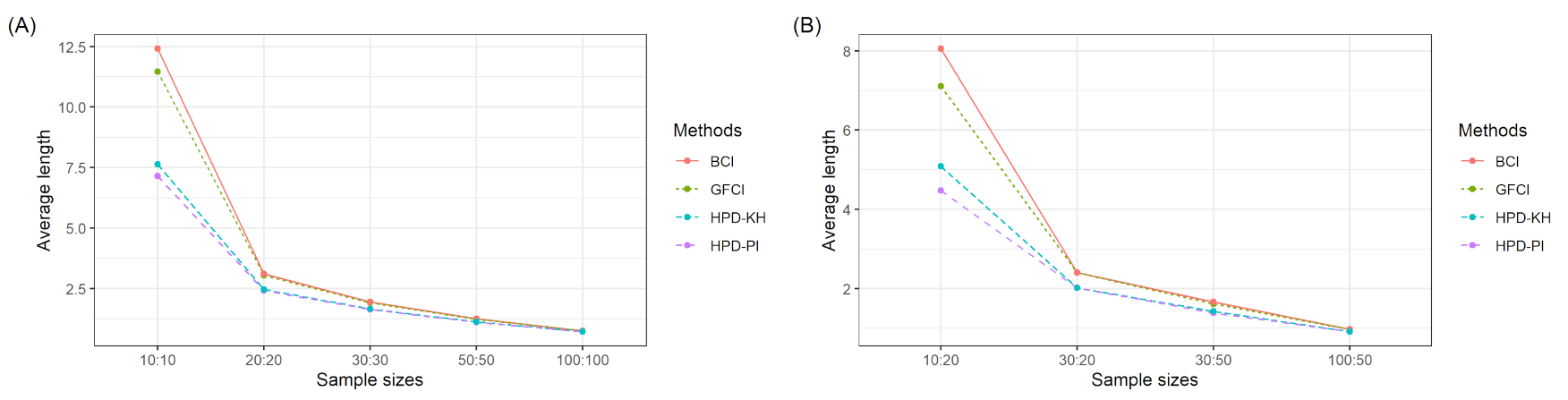
Table 1 and Table 2 report the simulation results, while Figure 1 and Figure 2 summarize the coverage probabilities and average lengths in Table 1 and Table 2. The simulation results from Table 1 and Table 2 indicate that the coverage probabilities of the four methods were greater than or close to 0.95 under all configurations. In addition, it was found that the differences in coverage probability among the four methods were very small. Moreover, HPD-PI provided the narrowest average lengths while BCI provided the longest ones under all circumstances. The average lengths of HPD-IP were mostly narrower than GFCI, while the average lengths of HPD-KH were mostly narrower than those of BCI. Moreover, the average length of the four methods decreased as the sample sizes ( n 1 , n 2 ) increased.

4. Application of the Methods to Real Fatigue Life Data

To illustrate the effectiveness of the confidence interval construction methods proposed in this study in a real-life scenario, we used real datasets concerning the fatigue life of 6061-T6 aluminum coupons that were cut parallel to the rolling direction and oscillated at 18 cycles per second [5]. As reported in Table 3, there are two groups consisting of 101 and 102 observations with maximum stress levels per cycle of 21,000 and 26,000 psi, respectively (the summary statistics of each group are provided in Table 4). Hence, the ratio of variances was 0.0254. We chose r i = 2 and a i = b i = c i = d i = 10 4 , where i = 1 , 2 , for the Bayesian credible interval and HPD-KH.
The results for the 95% confidence interval for the ratio of variances reported in Table 5 indicate that the length provided by HPD-PI was the narrowest while that of the Bayesian credible interval was the longest. These results are in accordance with those from the simulation studies where ( n 1 , n 2 ) = ( 100 , 100 ) . In addition, the confidence intervals constructed by using the various methods did not contain 1, and so it can be concluded that there is no significant difference in terms of variance for the fatigue lifetime of 6061-T6 aluminum coupons with maximum stress per cycle of 21,000 and 26,000 psi, respectively.

5. Conclusions

Four methods, namely GFCI, BCI, HPD-PI, and HPD-KH, were proposed for constructing the confidence interval for the ratio of variances of two BS distributions. A Monte Carlo simulation study was conducted to assess their performances based on their coverage probabilities and average lengths. The simulation study results indicate that the coverage probabilities of all of the methods were greater than or close to the nominal level of 0.95. However, HPD-PI outperformed the others by providing the narrowest average lengths in all of the scenarios studied. In addition, the results of using fatigue lifetime data of 6061-T6 aluminum coupons coincided with those from the simulation study. Therefore, HPD-PI can be recommended for constructing the confidence interval for the ratio of variances of two BS distributions.

Author Contributions

Conceptualization, S.N.; Data curation, W.P.; Formal analysis, W.P. and S.N.; Funding acquisition, S.N.; Investigation, S.-A.N. and S.N.; Methodology, S.-A.N. and S.N.; Project administration, S.-A.N.; Resources, S.-A.N.; Software, W.P.; Supervision, S.-A.N. and S.N.; Visualization, S.-A.N.; Writing original draft, W.P.; Writing–review & editing, S.-A.N. and S.N. All authors have read and agreed to the published version of the manuscript.

Funding

This research received financial support from the National Science, Research, and Innovation Fund (NSRF), and King Mongkut’s University of Technology North Bangkok (Grant No. KMUTNB–FF–65–23).

Institutional Review Board Statement

Not applicable.

Informed Consent Statement

Not applicable.

Data Availability Statement

The real data sets of the fatigue life of 6061-T6 aluminum coupons are available in the work of Birnbaum and Saunder [5].

Acknowledgments

The first author wishes to express gratitude for financial support provided by the Thailand Science Achievement Scholarship (SAST).

Conflicts of Interest

The authors declare no conflict of interest.

References

  1. Vassilopoulos, A.P. Fatigue life modeling and prediction methods for composite materials and structures—Past, present, and future prospects. In Fatigue Life Prediction of Composites and Composite Structures; Vassilopoulos, A.P., Ed.; Woodhead Publishing: Sawston, UK, 2020; pp. 1–43. [Google Scholar]
  2. Birnbaum, Z.W.; Saunders, S.C. A new family of life distributions. J. Appl. Probab. 1969, 6, 319–327. [Google Scholar] [CrossRef]
  3. Desmond, A.F. Stochastic models of failure in random environments. Can. J. Stat. 1985, 13, 171–183. [Google Scholar] [CrossRef]
  4. Desmond, A.F. On the relationship between two fatigue-life model. IEEE Trans. Reliab. 1986, 35, 167–169. [Google Scholar] [CrossRef]
  5. Birnbaum, Z.W.; Saunders, S.C. Estimation for a family of life distributions with applications to fatigue. J. Appl. Probab. 1969, 6, 328–347. [Google Scholar] [CrossRef]
  6. Aslam, M.; Jun, C.H.; Ahmad, M. New acceptance sampling plans based on life tests for Birnbaum-Saunders distributions. J. Stat. Comput. Simul. 2011, 81, 461–470. [Google Scholar] [CrossRef]
  7. Leiva, V.; Marchant, C.; Ruggeri, F.; Saulo, H. A criterion for environmental assessment using Birnbaum–Saunders attribute control charts. Environmetrics 2015, 26, 463–476. [Google Scholar] [CrossRef]
  8. Marchant, C.; Bertin, K.; Leiva, V.; Saulo, H. Generalized Birnbaum-Saunders kernel density estimators and an analysis of financial data. Comput. Stat. Data Anal. 2013, 63, 1–15. [Google Scholar] [CrossRef]
  9. Engelhardt, M.; Bain, L.J.; Wright, F.T. Inference on the parameters of the Birnbaum–Saunders fatigue life distribution based on maximum likelihood estimation. Technometrics 1981, 23, 251–255. [Google Scholar] [CrossRef]
  10. Achcar, J. Inferences for the Birnbaum-Saunders fatigue life model using Bayesian methods. Comput. Stat. Data Anal. 1993, 15, 367–380. [Google Scholar] [CrossRef]
  11. Ng, H.K.T.; Kundu, D.; Balakrishnan, N. Modified moment estimation for the two-parameter Birnbaum–Saunders distribution. Comput. Stat. Data Anal. 2003, 43, 283–298. [Google Scholar] [CrossRef]
  12. Lemonte, A.J.; Simas, A.B.; Cribari-Neto, F. Bootstrap-based improved estimators for the two-parameter Birnbaum–Saunders distribution. J. Stat. Comput. Simul. 2008, 78, 37–49. [Google Scholar] [CrossRef]
  13. Wang, B.X. Generalized interval estimation for the Birnbaum-Saunders distribution. Comput. Stat. Data Anal. 2012, 56, 4320–4326. [Google Scholar] [CrossRef]
  14. Xu, A.; Tang, Y. Reference analysis for Birnbaum-Saunders distribution. Comput. Stat. Data Anal. 2010, 54, 185–192. [Google Scholar] [CrossRef]
  15. Niu, C.; Guo, X.; Zhu, L. Comparison of several Birnbaum–Saunders distributions. J. Stat. Comput. Simul. 2014, 84, 2721–2733. [Google Scholar] [CrossRef]
  16. Wang, M.; Sun, X.; Park, C. Bayesian analysis of Birnbaum-Saunders distribution via the generalized ratio-of-uniforms method. Comput. Stat. 2016, 31, 207–225. [Google Scholar] [CrossRef]
  17. Li, Y.; Xu, A. Fiducial inference for Birnbaum-Saunders distribution. J. Stat. Comput. Simul. 2016, 86, 1673–1685. [Google Scholar] [CrossRef]
  18. Guo, X.; Wu, H.; Li, G.; Li, Q. Inference for the common mean of several Birnbaum–Saunders populations. J. Appl. Stat. 2017, 44, 941–954. [Google Scholar] [CrossRef]
  19. Puggard, W.; Niwitpong, S.A.; Niwitpong, S. Bayesian estimation for the coefficients of variation of Birnbaum-Saunders distributions. Symmetry 2021, 13, 2130. [Google Scholar] [CrossRef]
  20. Casella, G.; Berger, R.L. Statistical Inference; Thomson Learning: Boston, MA, USA, 2002. [Google Scholar]
  21. Bonett, D.G. Confidence interval for a ratio of variances in bivariate nonnormal distributions. J. Stat. Comput. Simul. 2006, 76, 637–644. [Google Scholar] [CrossRef]
  22. Bebu, I.; Mathew, T. Comparing the means and variances of a bivariate log-normal distribution. Stat. Med. 2008, 27, 2684–2696. [Google Scholar] [CrossRef]
  23. Paksaranuwat, P.; Niwitpong, S.A. Confidence intervals for the variance and the ratio of two variances of non-normal distributions with missing data. Thail. Stat. 2010, 8, 81–92. [Google Scholar]
  24. Niwitpong, S.A. Generalized confidence intervals for function of variances of lognormal distribution. Adv. Appl. Stat. 2017, 51, 151–163. [Google Scholar] [CrossRef]
  25. Wongyai, C.; Suwan, S. Comparisons of confidence interval for a ratio of non-normal variances using a kurtosis estimator. In Proceedings of the 12th International Conference of the Thailand Econometric Society (TES2019), Chiang Mai, Thailand, 9–11 January 2019. [Google Scholar]
  26. Maneerat, P.; Niwitpong, S.A.; Niwitpong, S. A Bayesian approach to construct confidence intervals for comparing the rainfall dispersion in Thailand. PeerJ 2020, 8, e8502. [Google Scholar] [CrossRef] [PubMed] [Green Version]
  27. Hannig, J. On generalized fiducial inference. Stat. Sin. 2009, 19, 491–544. [Google Scholar]
  28. Hannig, J. Generalized fiducial inference via discretization. Stat. Sin. 2013, 23, 489–514. [Google Scholar] [CrossRef]
  29. Gilks, W.R.; Wild, P. Adaptive rejection sampling for Gibbs sampling. J. Appl. Stat. 1992, 41, 337–348. [Google Scholar] [CrossRef]
  30. Gilks, W.R.; Best, N.G.; Tan, K.K.C. Adaptive rejection metropolis sampling within Gibbs sampling. J. Appl. Stat. 1995, 44, 455–472. [Google Scholar] [CrossRef] [Green Version]
  31. Wakefield, J.C.; Gelfand, A.E.; Smith, A.F.M. Efficient generation of random variates via the ratio-of-uniforms method. Stat. Comput. 1991, 1, 129–133. [Google Scholar] [CrossRef]
  32. Box, G.E.P.; Tiao, G.C. Bayesian Inference in Statistical Analysis; Wiley: New York, NY, USA, 1992. [Google Scholar]
Figure 1. A summary of the coverage probabilities of the methods in Table 1 and Table 2. (A) Equal sample sizes and (B) unequal sample sizes.
Symmetry 14 01492 g001
Figure 2. A summary of the average lengths of the methods in Table 1 and Table 2. (A) Equal sample sizes and (B) unequal sample sizes.
Symmetry 14 01492 g002
Table 1. Coverage probabilities and average lengths of the 95% confidence interval for the ratio of variances of two BS distributions with equal sample sizes ( n 1 = n 2 ) constructed via the various methods.
Coverage ProbabilityAverage Length
( n 1 , n 2 ) ( α 1 , α 2 )GFCIBCIHPD-PIHPD-KHGFCIBCIHPD-PIHPD-KH
(10, 10)(0.25, 0.25)0.9450.9500.9410.9436.06366.63954.78565.1260
(0.25, 0.50)0.9220.9390.9350.9411.48461.61601.16021.2418
(0.25, 1.00)0.9230.9250.9360.9460.39960.43110.30320.3231
(0.50, 0.50)0.9320.9440.9320.93811.44712.7468.03298.7739
(0.50, 1.00)0.9420.9490.9430.9492.48252.74331.72351.8892
(1.00, 1.00)0.9310.9350.9490.95146.84850.34526.87128.443
(20, 20)(0.25, 0.25)0.9400.9470.9480.9482.89543.00052.55082.6280
(0.25, 0.50)0.9250.9230.9370.9410.68260.70110.59690.6111
(0.25,1.00)0.9420.9440.9430.9500.14140.14500.12010.1227
(0.50, 0.50)0.9390.9400.9350.9394.35824.50503.61263.7198
(0.50, 1.00)0.9320.9420.9350.9390.88500.91490.71800.7383
(1.00, 1.00)0.9410.9460.9440.9529.27489.41426.85876.9256
(30, 30)(0.25, 0.25)0.9380.9390.9420.9412.03012.07601.85991.8937
(0.25, 0.50)0.9320.9320.9360.9400.49060.49880.44690.4524
(0.25, 1.00)0.9420.9450.9340.9340.09450.09600.08440.0851
(0.50, 0.50)0.9540.9580.9410.9452.75332.81412.42212.4720
(0.50, 1.00)0.9460.9530.9480.9520.56210.57130.48410.4910
(1.00, 1.00)0.9460.9450.9480.9475.58385.64714.49824.5328
(50, 50)(0.25, 0.25)0.9360.9360.9390.9411.44001.45641.36031.3747
(0.25, 0.50)0.9430.9470.9390.9380.33220.33540.31270.3156
(0.25, 1.00)0.9540.9570.9530.9560.06580.06630.06100.0613
(0.50, 0.50)0.9530.9550.9450.9511.94501.96741.79171.8075
(0.50, 1.00)0.9540.9530.9460.9460.35090.35480.31870.3212
(1.00, 1.00)0.9480.9520.9440.9443.28063.28752.83412.8475
(100, 100)(0.25,0.25)0.9450.9490.9480.9360.95180.95580.91970.9242
(0.25, 0.50)0.9490.9530.9370.9430.21750.21830.21020.2106
(0.25, 1.00)0.9640.9590.9640.9620.04230.04240.04050.0406
(0.50, 0.50)0.9380.9340.9430.9511.23081.23991.17571.1813
(0.50, 1.00)0.9410.9470.9540.9560.22650.22700.21440.2151
(1.00, 1.00)0.9530.9520.9530.9561.84451.85321.70341.7082
GFCI, the generalized fiducial confidence interval; BCI, the Bayesian credible interval; HPD-PI, the highest posterior density interval based on a prior with partial information; HPD-KH, the highest posterior density interval based on the proper prior with known hyperparameters.
Table 2. Coverage probabilities and average lengths of the 95% confidence interval for the ratio of variances of two BS distributions with unequal sample sizes ( n 1 n 2 ) constructed via the various methods.
Coverage ProbabilityAverage Length
( n 1 , n 2 ) ( α 1 , α 2 )GFCIBCIHPD-PIHPD-KHGFCIBCIHPD-PIHPD-KH
(10,20)(0.25,0.25)0.9430.9530.9270.9414.20724.86703.34133.7992
(0.25,0.50)0.9300.9380.9240.9381.03681.18810.82140.9220
(0.25,1.00)0.9330.9480.9310.9460.19350.21840.15060.1679
(0.50,0.50)0.9260.9400.9220.9378.19249.60885.77586.7158
(0.50,1.00)0.9450.9520.9380.9541.43231.67451.01121.1602
(1.00,1.00)0.9350.9480.9300.94927.60130.80115.72817.728
(30,20)(0.25,0.25)0.9480.9510.9460.9532.43092.46422.21962.2377
(0.25,0.50)0.9390.9440.9580.9540.59100.59200.53420.5325
(0.25,1.00)0.9450.9480.9400.9470.12730.12730.11130.1107
(0.50,0.50)0.9360.9370.9390.9463.42943.45492.99053.0062
(0.50,1.00)0.9400.9470.9520.9520.69150.69530.58650.5876
(1.00,1.00)0.9460.9470.9490.9497.14867.09665.67075.6205
(30,50)(0.25,0.25)0.9510.9520.9490.9521.81531.87671.66451.7200
(0.25,0.50)0.9360.9380.9360.9450.40300.41440.36830.3779
(0.25,1.00)0.9430.9460.9440.9500.07430.07640.06720.0689
(0.50,0.50)0.9520.9540.9450.9552.44222.53892.15442.2279
(0.50,1.00)0.9540.9530.9500.9550.44750.46330.39150.4032
(1.00,1.00)0.9450.9470.9420.9454.49384.61073.65593.7389
(100,50)(0.25,0.25)0.9360.9370.9360.9331.18481.18301.14261.1422
(0.25,0.50)0.9420.9470.9470.9450.28730.28580.27590.2741
(0.25,1.00)0.9450.9440.9430.9380.05810.05770.05470.0544
(0.50,0.50)0.9390.9420.9410.9361.55331.55551.47791.4747
(0.50,1.00)0.9470.9510.9490.9480.30590.30390.28540.2832
(1.00,1.00)0.9590.9570.9560.9542.45642.44782.23282.2283
GFCI, the generalized fiducial confidence interval; BCI, the Bayesian credible interval; HPD-PI, the highest posterior density interval based on a prior with partial information; HPD-KH, the highest posterior density interval based on the proper prior with known hyperparameters.
Table 3. Fatigue lifetime data of 6061-T6 aluminum coupons.
Group 1370706716746785797844855858886886
9309609889901000101010161018102010551085
11021102110811151120113411401199120012001203
12221235123812521258126212691270129012931300
13101313131513301355139014161419142014201450
14521475147814811485150215051513152215221530
15401560156715781594160216041608163016421674
17301750175017631768178117821792182018681881
18901893189519101923194019452023210021302215
22682440
Group 2233258268276290310312315318321321
329335336338338342342342344349350
350351351352352356358358360362363
366367370370372372374375376379379
380382389389395396400400400403404
406408408410412414416416416420422
423426428432432433433437438439439
443445445452456456460464466468470
470473474476476486488489490491503
517540560
Table 4. Summary statistics for the fatigue lifetime data of 6061-T6 aluminum coupons.
GroupnMin.MedianMeanMax.Variance
110137014161400.91102440153,134.5
2102233400397.88245603834.3030
Table 5. The 95% confidence interval for the ratio of variances of the fatigue lifetime data of 6061-T6 aluminum coupons with maximum stress levels per cycle of 21,000 and 26,000 psi.
MethodsIntervalLength
GFCI0.0138–0.03320.0193
BCI0.0138–0.03370.0199
HPD-PI0.0132–0.03150.0184
HPD-KH0.0126–0.03150.0189
GFCI, the generalized fiducial confidence interval; BCI, the Bayesian credible interval; HPD-PI, the highest posterior density interval based on a prior with partial information; HPD-KH, the highest posterior density interval based on the proper prior with known hyperparameters.
Publisher’s Note: MDPI stays neutral with regard to jurisdictional claims in published maps and institutional affiliations.

