Reconstructing the Unknown Source Function of a Fractional Parabolic Equation from the Final Data with the Conformable Derivative

Abstract

The paper’s main purpose is to find the unknown source function for the conformable heat equation. In the case of $(\mathrm{\Phi },g)\in {\mathcal{L}}^2(0,T)\times {\mathcal{L}}^2\left(\mathrm{\Omega }\right)$, we give a modified Fractional Landweber solution and explore the error between the approximate solution and the desired solution under a priori and a posteriori parameter choice rules. The error between the regularized and exact solution is then calculated in ${\mathcal{L}}^q\left(\mathcal{D}\right)$, with $q\ne 2$ under some reasonable Cauchy data assumptions.

1. Introduction

In this paper, we consider the initial value problem for the conformable heat equation (or called parabolic equation with conformable operator):

$$\left\{\begin{array}{cc}{\displaystyle \frac{{}^C{\partial }^{\beta }}{\partial t^{\beta }}\left(u-k\Delta u\right)-\Delta u(x,t)=\mathrm{\Phi }\left(t\right)f\left(x\right),}\hfill & x\in \mathcal{D},t\in (0,T),\hfill \\ u(x,t)=0,\hfill & x\in \partial \mathcal{D},t\in (0,T).\hfill \end{array}\right.$$

(1)

Here, $\mathcal{D}\subset {\mathbb{R}}^N$ ($N\ge 1$) is a bounded domain with the smooth boundary $\partial \mathcal{D}$, and $T>0$. It is an obvious fact that a conformable operator has many practical applications, branches of science and engineering; see for example [1,2,3,4,5,6,7,8,9,10]. The applications of conformable derivative models in the harmonic oscillator include the damped oscillator, and the forced oscillator (see [11]), electrical circuits (see [12]), chaotic systems in dynamics (see [13]), and many more applications, (see [14,15,16,17,18,19,20,21]).

Conformable derivative model: Let us take B as a Banach space, and f as a B-valued function on $[0,\infty )$. Let $\frac{{}^C{\partial }^{\beta }}{\partial t^{\beta }}$ be the conformable derivative of order $0<\beta \le 1$ locally defined by:

$$\frac{{}^C{\partial }^{\beta }f\left(t\right)}{\partial t^{\beta }}:=\underset{\tau \to 0}{lim}\frac{f(t+\tau t^{1-\beta })-f\left(t\right)}{\tau }\mathrm{in}B,$$

for each $t>0$. For more knowledge about the above definition, we refer the reader to [22,23,24]. There are two interesting points regarding the relationship between conformable and classical derivatives:

• Let us assume that $B\equiv \mathbb{R}$, if f is a real function and $s>0$, then f has a conformable fractional derivative of order $\beta$, and $\frac{{}^C{\partial }^{\beta }f\left(s\right)}{\partial s^{\beta }}=s^{1-\beta }\frac{\partial f\left(s\right)}{\partial s};$
• If B is not $\mathbb{R}$, for example B are Sobolev spaces. There are not many conformable related results in Banach spaces, see [25].

The inverse source problem for (1) is described as follows. The final time condition $u(x,T)=g\left(x\right),$ together with the additional condition $u(x,0)=0,x\in \mathcal{D}$. The inverse source problem for (1) is understood as finding the function f when the input data $g,\mathrm{\Phi }$ is given. As we know, the Problem (1) is ill-posed, and according to our experience and understanding, the frequent infringement is the continuity of the solution according to data. Therefore, to provide a good approximation, we need to regularize these problems. Before going into adjustment, we would like to review a bit of the history of the Problem (1).

• In case $\beta =1$, the above equation becomes the classical pseudo-parabolic equation; this type of equation has received much attention from mathematicians, see [26,27,28];
• In case $\beta \ne 1$, with Caputo derivative model, we find the following documents, see [4]. Luc and co-authors studied the existence and uniqueness of a class of mild solutions of these equations. In [29], the authors considered the non-local Problem (1) for a pseudo-parabolic equation with fractional time and space. In [30], Tuan and his group considered a class of pseudoparabolic equations with the nonlocal condition in two cases: the nonlinear source function ad linear source function. For the first case, by using the Sobolev embeddings, they established the existence, the uniqueness, and some regularity results for the mild solution of Problem (1). For the second case, using the Banach fixed-point theorem, they proved the existence and the uniqueness of the mild solution for (1). In [31], the authors considered two problems. For the first problem with the source term satisfying the globally Lipschitz condition, we establish the local well-posedness theory, and the further local existence theory related to the finite time blow-up are also obtained for the problem with logarithmic nonlinearity. For the second problem, they proved the global existence theorem.
• We have not seen any findings for this kind in case $\beta \ne 1$ with the conformable derivative model, and the source function survey problem is much more sparse, thus our study concentrates on this topic.

The regularization problem is a very interesting problem, with common regularization methods such as the Tikhonov method [32], Quasi Boundary Value method [33], Fractional Tikhonov method [34] and mollification method [35]. In [36], T. Wei with the Tikhonov regularization method, in [37], Ting Wei and her group considered a time-dependent source term by using a boundary element method combined with a generalized Tikhonov regularization. However, in this article, we use a modified fractional Landweber method to solve the unknown source Problem (1). Besides, there is a new point in this paper; we evaluate the error of exact and normalized solutions in ${\mathcal{L}}^q\left(\mathcal{D}\right)$ space, with $q\ne 2$. In this case, the equality Parseval was not used. One way to overcome this weakness is to use the embedding between ${\mathcal{L}}^q\left(\mathcal{D}\right)$ and Hilbert scales spaces ${\mathbb{X}}^r\left(\mathcal{D}\right)$. The main analytical technique in our paper is to use some embeddings and some analysis estimators related to Hölder inequality. To complete our proofs, we learn many interesting techniques from N.H. Tuan [38]. For the reader’s convenience, we would like to outline the main results of the paper.

• We give the ill-posedness of Problem (1);
• Showing the regularization of Problem (1), with the two subsections;

  -

  Uncertainty of Problem (1) of determining the source function;

  -

  The conditional stability of Problem (1);

• Using the modified fractional Landweber method to solve the Problem (1). We obtain the convergence rate as follows:

  -

  In Section 4.1, under a priori parameter choice rule;

  -

  In Section 4.2, under a posteriori parameter choice rule.

• It gives the error estimate in ${\mathcal{L}}^q$ space, with $q\ne 2$.

This paper is organized as follows. Section 2 introduces some function spaces and embeddings. In Section 4, we deal with the regularized solution for the inverse source problem for (1) by the Modified Fractional Landweber method under a priori and a posteriori parameter choice rules. In Section 5, we solve the Problem (1) in the case of observed data in ${\mathcal{L}}^q$ space. Finally, we present a numerical experiment.

2. Preliminary Results

Let us recall that the spectral problem:

$$\begin{array}{c}\hfill \left\{\begin{array}{cc}\Delta {\mathit{e}}_n\left(x\right)=-{\lambda }_n{\mathit{e}}_n\left(x\right),\hfill & x\in \mathcal{D},\hfill \\ {\mathit{e}}_n\left(x\right)=0,\hfill & x\in \partial D,\hfill \end{array}\right.\end{array}$$

admits the eigenvalues $0<{\lambda }_1\le {\lambda }_2\le \cdots \le {\lambda }_n\le \cdots$ with ${\lambda }_n\to \infty$ as $n\to \infty$. The corresponding eigenfunctions are ${\psi }_n\in H_0^1\left(\mathrm{\Omega }\right)$.

Definition 1.

(Hilbert scale space). We recall the Hilbert scale space, which is given as follows:

$$\begin{array}{c}\hfill {\mathbb{X}}^r\left(\mathcal{D}\right)=\left\{f\in L^2\left(\mathcal{D}\right),\sum _{n=1}^{\infty }{\lambda }_n^{2r}{\left({\int }_{\mathcal{D}}f\left(x\right){\mathit{e}}_n\left(x\right)dx\right)}^2<\infty \right\},\end{array}$$

for any $r\ge 0$. It is well-known that ${\mathbb{X}}^r\left(\mathcal{D}\right)$ is a Hilbert space corresponding to the norm,

$$\begin{array}{c}\hfill {\parallel f\parallel }_{{\mathbb{X}}^r\left(\mathcal{D}\right)}={\left(\sum _{n=1}^{\infty }{\lambda }_n^{2r}{\left({\int }_{\mathcal{D}}f\left(x\right){\mathit{e}}_n\left(x\right)dx\right)}^2\right)}^{1/2},f\in {\mathbb{X}}^r\left(\mathcal{D}\right).\end{array}$$

(2)

Lemma 1.

 Let $\mathrm{\Phi }:[0,T]\to \mathbb{R}$ such that ${\mathrm{\Phi }}_0\le \mathrm{\Phi }\left(t\right)\le {\mathrm{\Phi }}_1$ where ${\mathrm{\Phi }}_0$ and ${\mathrm{\Phi }}_1$ are positive numbers. Then the following estimates are true:

$$\frac{1}{1+k{\lambda }_n}{\int }_0^T{s}^{\beta -1}exp\left(\frac{{\lambda }_n}{1+k{\lambda }_n}\frac{s^{\beta }-T^{\beta }}{\beta }\right)\mathrm{\Phi }\left(s\right)ds\le \frac{T^{\beta }}{\beta }\frac{{\mathrm{\Phi }}_1}{{\lambda }_n},$$

(3)

and

$$\frac{{\mathrm{\Phi }}_0}{{\lambda }_n}\left[1-exp\left(-\frac{{\lambda }_1}{1+k{\lambda }_1}\frac{T^{\beta }}{\beta }\right)\right]\le \frac{1}{1+k{\lambda }_n}{\int }_0^T{s}^{\beta -1}exp\left(\frac{{\lambda }_n}{1+k{\lambda }_n}\frac{s^{\beta }-T^{\beta }}{\beta }\right)\mathrm{\Phi }\left(s\right)ds.$$

(4)

Proof. 

First of all, we have the estimate ${\int }_0^T{s}^{\beta -1}exp\left(\frac{{\lambda }_n}{1+k{\lambda }_n}\frac{s^{\beta }-T^{\beta }}{\beta }\right)ds=exp\left(-\frac{{\lambda }_n}{1+k{\lambda }_n}\frac{T^{\beta }}{\beta }\right)\underset{0}{\overset{T}{\int }}{s}^{\beta -1}exp\left(\frac{{\lambda }_n}{1+k{\lambda }_n}\frac{s^{\beta }}{\beta }\right)ds$, putting $z=\frac{{\lambda }_n}{1+k{\lambda }_n}\frac{s^{\beta }}{\beta }$, and through basic calculations, and applying the inequality $(1-e^{-x})\le x$, for $x\ge 0$, since $\mathrm{\Phi }\left(t\right)\le {\mathrm{\Phi }}_1$, we get:

$$\begin{array}{c}\hfill \frac{1}{1+k{\lambda }_n}{\int }_0^T{s}^{\beta -1}exp\left(\frac{{\lambda }_n}{1+k{\lambda }_n}\frac{s^{\beta }-T^{\beta }}{\beta }\right)\mathrm{\Phi }\left(s\right)ds\le \frac{T^{\beta }}{\beta }\frac{{\mathrm{\Phi }}_1}{{\lambda }_n}·.\end{array}$$

(5)

Since $\mathrm{\Phi }\left(t\right)\ge {\mathrm{\Phi }}_0>0$, we have:

$$\begin{array}{cc}\hfill \frac{1}{1+k{\lambda }_n}\underset{0}{\overset{T}{\int }}{s}^{\beta -1}exp\left(\frac{{\lambda }_n}{1+k{\lambda }_n}\frac{s^{\beta }-T^{\beta }}{\beta }\right)\mathrm{\Phi }\left(s\right)ds& \ge {\mathrm{\Phi }}_0\underset{0}{\overset{T}{\int }}{s}^{\beta -1}exp\left(\frac{{\lambda }_n}{1+k{\lambda }_n}\frac{s^{\beta }-T^{\beta }}{\beta }\right)ds\hfill \\ \hfill & =\frac{{\mathrm{\Phi }}_0}{{\lambda }_n}\left[1-exp\left(-\frac{{\lambda }_1}{1+k{\lambda }_1}\frac{T^{\beta }}{\beta }\right)\right].\hfill \end{array}$$

(6)

Let us consider the following function: $G\left(x\right)={\displaystyle \frac{x}{1+kx}},x>0.$ The derivative of which is equal to: $G^{\prime }\left(x\right)={\displaystyle \frac{1}{{(1+kx)}^2}}>0.$ This implies that G is an increasing function on $(0,+\infty )$. Therefore, we get:

$${\lambda }_n{\left(1+k{\lambda }_n\right)}^{-1}\ge {\lambda }_1{\left(1+k{\lambda }_1\right)}^{-1}.$$

It follows from (6) that:

$$\begin{array}{c}\hfill \frac{1}{1+k{\lambda }_n}\underset{0}{\overset{T}{\int }}{s}^{\beta -1}exp\left(\frac{{\lambda }_n}{1+k{\lambda }_n}\frac{s^{\beta }-T^{\beta }}{\beta }\right)\mathrm{\Phi }\left(s\right)ds\ge \frac{{\mathrm{\Phi }}_0}{{\lambda }_n}\left[1-exp\left(-\frac{{\lambda }_1}{1+k{\lambda }_1}\frac{T^{\beta }}{\beta }\right)\right].\end{array}$$

(7)

The Lemma is proven. □

Lemma 2.

Let ${\mathrm{\Phi }}_0,{\mathrm{\Phi }}_1$ be positive constants such that ${\mathrm{\Phi }}_0<\mathrm{\Phi }\left(t\right)<{\mathrm{\Phi }}_1$. By choosing

$\delta \in \left(0,{\displaystyle \frac{{\mathrm{\Phi }}_1}{4}}\right)$, and $\mathcal{B}({\mathrm{\Phi }}_0,{\mathrm{\Phi }}_1)={\mathrm{\Phi }}_1+{\displaystyle \frac{{\mathrm{\Phi }}_0}{4}}$, we obtain

$$\begin{array}{c}\hfill 4^{-1}{\mathrm{\Phi }}_0\le |{\mathrm{\Phi }}_{\delta }\left(t\right)|\le \mathcal{B}\left({\mathrm{\Phi }}_0,{\mathrm{\Phi }}_1\right)·\end{array}$$

(8)

Proof. 

See in [39]. □

Lemma 3.

(See [40]) The following statements are true:

$$\begin{array}{c}\hfill \left.\begin{array}{c}{\displaystyle L^p\left(\mathcal{D}\right)\hookrightarrow {\mathbb{X}}^{\mu }\left(\mathcal{D}\right),\mathrm{if}-\frac{N}{4}<\mu \le 0,p\ge \frac{2N}{N-4\mu },}\hfill \\ {\displaystyle {\mathbb{X}}^s\left(\mathcal{D}\right)\hookrightarrow L^p\left(\mathcal{D}\right),\mathrm{if}0\le s<\frac{N}{4},p\le \frac{2N}{N-4s}.}\hfill \end{array}\right\}\end{array}$$

(9)

3. Regularization of Inverse Source Problem

We consider the mild solution in Fourier series, ${\displaystyle u(x,t)=\sum _{n=1}^{\infty }{u}_n\left(t\right){\mathit{e}}_n\left(x\right)}$, with $u_n\left(t\right)=\underset{\mathcal{D}}{\int }u(·,t){\mathit{e}}_n\left(x\right)dx$. Taking the inner product of the equations of Problem (1) with ${\mathit{e}}_n$ gives:

$$\begin{array}{c}\hfill \left\{\begin{array}{ccc}{\displaystyle \frac{{}^C{\partial }^{\beta }}{\partial t^{\beta }}⟨u(.,t),{\mathit{e}}_n⟩+k{\lambda }_n\frac{{}^C{\partial }^{\beta }}{\partial t^{\beta }}⟨u(.,t),{\mathit{e}}_n⟩-{\lambda }_n⟨u(.,t),{\mathit{e}}_n⟩}\hfill & =⟨F(.,t),{\mathit{e}}_n⟩,\hfill & t\in (0,T),\hfill \\ ⟨u(.,0),e_n⟩\hfill & =⟨u_0,e_n⟩\hfill & .\hfill \end{array}\right.\end{array}$$

(10)

The first equation of (10) is a differential equation with a conformable derivative as follows:

$${\displaystyle \frac{{}^C{\partial }^{\beta }}{\partial t^{\beta }}{u}_n\left(t\right)-\frac{{\lambda }_n}{1+k{\lambda }_n}{u}_n\left(t\right)=\frac{1}{1+k{\lambda }_n}{F}_n\left(t\right).}$$

(11)

In view of the result in (Theorem 5, “[41], p. 318”) and (Theorem 3.3, “[42], p. 318”), the solution of Problem (1) is:

$$\begin{array}{c}\hfill u_n\left(t\right)=exp\left(-\frac{{\lambda }_n}{1+k{\lambda }_n}\frac{t^{\beta }}{\beta }\right)u_{0,n}+\frac{1}{1+k{\lambda }_n}{\int }_0^t{s}^{\beta -1}exp\left(\frac{{\lambda }_n}{1+k{\lambda }_n}\frac{s^{\beta }-t^{\beta }}{\beta }\right)F_n\left(s\right)ds.\end{array}$$

To find the formula of the mild solution to Problem (1), with $u_n\left(0\right)=0$ and $F_n\left(s\right)=\mathrm{\Phi }\left(s\right)f\left(x\right)$. Letting $t=T$, we know that:

$$\begin{array}{c}\hfill \left(\underset{\mathcal{D}}{\int }g\left(x\right){\mathit{e}}_n\left(x\right)dx\right)=\frac{1}{1+k{\lambda }_n}\left(\underset{\mathcal{D}}{\int }f\left(x\right){\mathit{e}}_n\left(x\right)dx\right)\underset{0}{\overset{T}{\int }}{s}^{\beta -1}exp\left(\frac{{\lambda }_n}{1+k{\lambda }_n}\frac{s^{\beta }-T^{\beta }}{\beta }\right)\mathrm{\Phi }\left(s\right)ds.\end{array}$$

(12)

After a simple transformation, we get:

$$\begin{array}{c}\hfill {\displaystyle \left(\underset{\mathcal{D}}{\int }f\left(x\right){\mathit{e}}_n\left(x\right)dx\right)={\left[\underset{0}{\overset{T}{\int }}{s}^{\beta -1}exp\left(\frac{{\lambda }_n}{1+k{\lambda }_n}\frac{s^{\beta }-T^{\beta }}{\beta }\right)\mathrm{\Phi }\left(s\right)ds\right]}^{-1}\left(1+k{\lambda }_n\right)\left(\underset{\mathcal{D}}{\int }g\left(x\right){\mathit{e}}_n\left(x\right)dx\right).}\end{array}$$

(13)

This leads to:

$$\begin{array}{c}\hfill {\displaystyle f\left(x\right)=\sum _{n=1}^{+\infty }{\left[\underset{0}{\overset{T}{\int }}{s}^{\beta -1}exp\left(\frac{{\lambda }_n}{1+k{\lambda }_n}\frac{s^{\beta }-T^{\beta }}{\beta }\right)\mathrm{\Phi }\left(s\right)ds\right]}^{-1}\left(1+k{\lambda }_n\right)\left(\underset{\mathcal{D}}{\int }g\left(x\right){\mathit{e}}_n\left(x\right)dx\right){\mathit{e}}_n\left(x\right).}\end{array}$$

(14)

3.1. Uncertainty of Source Problem

Theorem 1.

 The inverse source problem (1) is ill-posed.

Proof of Theorem 1. 

We defined a linear operator $\mathcal{S}:{\mathcal{L}}^2\left(\mathcal{D}\right)\to {\mathcal{L}}^2\left(\mathcal{D}\right)$ as follows.

$$\begin{array}{c}\hfill {\displaystyle \mathcal{S}f\left(x\right)=\sum _{n=1}^{+\infty }{(1+k{\lambda }_n)}^{-1}\left[\underset{0}{\overset{T}{\int }}{s}^{\beta -1}exp\left(\frac{{\lambda }_n}{1+k{\lambda }_n}\frac{s^{\beta }-T^{\beta }}{\beta }\right)\mathrm{\Phi }\left(s\right)ds\right]=\underset{\mathcal{D}}{\int }k(x,\omega )f\left(\omega \right)d\omega ,}\end{array}$$

(15)

where ${\displaystyle k(x,\omega )=\sum _{n=1}^{+\infty }{(1+k{\lambda }_n)}^{-1}\left[\underset{0}{\overset{T}{\int }}{s}^{\beta -1}exp\left(\frac{{\lambda }_n}{1+k{\lambda }_n}\frac{s^{\beta }-T^{\beta }}{\beta }\right)\mathrm{\Phi }\left(s\right)ds\right]{\mathit{e}}_n\left(x\right){\mathit{e}}_n\left(\omega \right).}$

Due to $k(x,\omega )=k(\omega ,x)$, $\mathcal{S}$ is a self-adjoint operator. We defined the finite rank operators ${\mathcal{S}}_{\mathcal{N}}$ and considered its compactness:

$${\displaystyle {\mathcal{S}}_{\mathcal{N}}f\left(x\right)=\sum _{n=1}^{\mathcal{N}}{(1+k{\lambda }_n)}^{-1}\left[\underset{0}{\overset{T}{\int }}{s}^{\beta -1}exp\left(\frac{{\lambda }_n}{1+k{\lambda }_n}\frac{s^{\beta }-T^{\beta }}{\beta }\right)\mathrm{\Phi }\left(s\right)ds\right]\left(\underset{\mathcal{D}}{\int }f\left(x\right){\mathit{e}}_n\left(x\right)dx\right){\mathit{e}}_n\left(x\right).}$$

(16)

From (16), through some basic calculations and using the Lemma 1, we have:

$$\begin{array}{c}\hfill \parallel {\mathcal{S}}_{\mathcal{N}}f-\mathcal{S}f{\parallel }_{{\mathcal{L}}^2\left(\mathcal{D}\right)}^2\le \frac{T^{\beta }{\mathrm{\Phi }}_1}{\beta }\sum _{n=\mathcal{N}+1}^{+\infty }\frac{1}{{\lambda }_n^2}{\left(\underset{\mathcal{D}}{\int }f\left(x\right){\mathit{e}}_n\left(x\right)dx\right)}^2.\end{array}$$

(17)

From (17), we have:

$$\parallel {\mathcal{S}}_{\mathcal{N}}f-\mathcal{S}f{\parallel }_{{\mathcal{L}}^2\left(\mathcal{D}\right)}^2\le {\left(\frac{T^{\beta }{\mathrm{\Phi }}_1}{\beta }\right)}^2\frac{1}{{\mathcal{N}}^2}\parallel f{\parallel }_{{\mathcal{L}}^2\left(\mathcal{D}\right)}^{2}to0in\mathcal{L}({\mathcal{L}}^2\left(\mathcal{D}\right);{\mathcal{L}}^2\left(\mathcal{D}\right))as\mathcal{N}\to \infty .$$

(18)

Additionally, $\mathcal{S}$ is a compact operator. The SVDs for the linear self-adjoint compact operator $\mathcal{S}$ are:

$${\displaystyle \mathcal{S}={(1+k{\lambda }_n)}^{-1}\left[\underset{0}{\overset{T}{\int }}{s}^{\beta -1}exp\left(\frac{{\lambda }_n}{1+k{\lambda }_n}\frac{s^{\beta }-T^{\beta }}{\beta }\right)\mathrm{\Phi }\left(s\right)ds\right],}$$

(19)

and corresponding eigenvectors are ${\mathit{e}}_n$ is an orthonormal basis in ${\mathcal{L}}_2\left(\mathcal{D}\right)$. Therefore, the inverse source Problem (1) can be formulated as an operator equation $\mathcal{S}f\left(x\right)=g\left(x\right)$ where, by $g\left(x\right)$, and by Kirsch, it is ill-posed. Next, we show an example, with final time data $g_i={\lambda }_i^{-\frac{1}{2}}{\mathit{e}}_i$ and $u_0=0$. By (14), the source term corresponding to $g_i$ is:

$$\begin{array}{cc}\hfill f_i\left(x\right)& {\displaystyle ={\left[\underset{0}{\overset{T}{\int }}{s}^{\beta -1}exp\left(\frac{{\lambda }_i}{1+k{\lambda }_i}\frac{s^{\beta }-T^{\beta }}{\beta }\right)\mathrm{\Phi }\left(s\right)ds\right]}^{-1}}\hfill \\ & \times (1+k{\lambda }_i)\left(\underset{\mathcal{D}}{\int }g\left(x\right){\mathit{e}}_i\left(x\right)dx\right){\mathit{e}}_i\left(x\right)\ge \frac{\beta {\lambda }_i^{\frac{1}{2}}}{T^{\beta }{\mathrm{\Phi }}_1}·\hfill \end{array}$$

(20)

The input final data $g=0$ then the source term corresponding to g is $f=0$. We have error in ${\mathcal{L}}^2$ norm between $g_i$ and g,

$$\underset{i\to +\infty }{lim}{\parallel g_i-g\parallel }_{{\mathcal{L}}^2\left(\mathcal{D}\right)}=\underset{i\to +\infty }{lim}{\lambda }_i^{-\frac{1}{2}}=0.$$

(21)

Then the error in ${\mathcal{L}}^2$ norm between $f_i$ and f

$$\parallel f_i-f{\parallel }_{{\mathcal{L}}^2\left(\mathcal{D}\right)}\ge \frac{\beta }{T^{\beta }{\mathrm{\Phi }}_1}{\lambda }_i^{\frac{1}{2}}⟶\underset{i\to +\infty }{lim}\parallel f_i-f{\parallel }_{{\mathcal{L}}^2\left(\mathcal{D}\right)}\ge +\infty .$$

(22)

From (21) and (22), we deduce that the solution to Problem (1) is unstable in ${\mathcal{L}}^2\left(\mathcal{D}\right)$. □

3.2. The Conditional Stability

Theorem 2. 

Assume that $f\in {\mathbb{X}}^r\left(\mathcal{D}\right)$, $g\in {\mathcal{L}}^2\left(\mathcal{D}\right)$, and ${\parallel f\parallel }_{{\mathbb{X}}^r\left(\mathcal{D}\right)}\le \mathcal{B}$ then we have:

$${\parallel f\parallel }_{{\mathcal{L}}^2\left(\mathcal{D}\right)}\le \overline{C}(m,\mathcal{B})\parallel g{\parallel }_{{\mathcal{L}}^2\left(\mathcal{D}\right)}^{\frac{r}{r+1}},$$

(23)

whereby $\overline{C}(r,\mathcal{B})={\mathcal{B}}^{\frac{1}{r+1}}|{\mathrm{\Phi }}_0\left(1-exp\left(-{\lambda }_1{(1+k{\lambda }_1)}^{-1}\frac{T^{\beta }}{\beta }\right)\right){|}^{-\frac{r}{r+1}}.$

Proof of Theorem 2. 

The proof of this theorem can be conducted similar to the articles [39]. We omit this here. □

4. A Modified Fractional Landweber Method and Convergent Rate

Based on a modified Fractional Landweber method, we show the error estimate under the a priori regularization parameter choice rule and the a-posteriori regularization parameter choice rule, respectively. Now, we use the modified Fractional Landweber iterative method to obtain the regularization solution for Problem (1). We give the following iterative form:

$$\begin{array}{c}\hfill f_0\left(x\right):=0,f_{\tau }\left(x\right)=f_{\tau -1}\left(x\right)-\xi \left({(\mathcal{S}*\mathcal{S})}^{\frac{\alpha +1}{2}}{f}_{\tau -1}\left(x\right)-{(\mathcal{S}*\mathcal{S})}^{\frac{\alpha -1}{2}}\mathcal{S}*g\left(x\right)\right),\tau =1,2,3,\cdots ,\end{array}$$

(24)

where $\tau$ is the iterative step number and the regularization parameter is ${\tau }^{-1}$. The coefficient $\xi$ is called the relaxation factor and satisfies ${0<\xi <\parallel \mathcal{S}\parallel }^{-(\alpha +1)}$, by denoting an operator $R_{\tau }:g\to f$ such that

$$\begin{array}{c}\hfill f_m\left(x\right)=\xi \sum _{k=0}^{m-1}(I-\xi {\left(\mathcal{S}*{\mathcal{S})}^{\frac{\alpha +1}{2}}\right)}^k(\mathcal{S}*{\mathcal{S})}^{\frac{\alpha -1}{2}}\mathcal{S}*g\left(x\right),\end{array}$$

(25)

with (19), it gives:

$$\begin{array}{c}\hfill f_{m,\delta }\left(x\right)={\mathcal{R}}_m{g}_{\delta }\left(x\right)=\sum _{n=1}^{+\infty }\frac{1-{\left(1-\xi |Q{\lambda }_n^{-1}{|}^{\alpha +1}\right)}^m}{{\mathcal{P}}_n(k,\beta ,T,{\mathrm{\Phi }}_{\delta })}\left(\underset{\mathcal{D}}{\int }{g}_{\delta }\left(x\right){\mathit{e}}_n\left(x\right)dx\right){\mathit{e}}_n\left(x\right),\end{array}$$

(26)

whereby

$$\begin{array}{c}\hfill {\mathcal{P}}_n(k,\beta ,T,{\mathrm{\Phi }}_{\delta })={(1+k{\lambda }_n)}^{-1}\left[\underset{0}{\overset{T}{\int }}{s}^{\beta -1}exp\left(\frac{{\lambda }_n}{1+k{\lambda }_n}\frac{s^{\beta }-T^{\beta }}{\beta }\right)\mathrm{\Phi }\left(s\right)ds\right].\end{array}$$

(27)

Lemma 4.

 For $0<\alpha <1$, if we choose $\xi \in \left(0,|{\displaystyle \frac{{\lambda }_1}{Q}}{|}^{\alpha +1}\right)$ then $0<\xi |{\displaystyle \frac{Q}{{\lambda }_1}}{|}^{\alpha +1}<1$, inwhich Q depends on $Q=T^{\beta }{\mathrm{\Phi }}_1{\beta }^{-1}$. With how to choose ξ in above, by denoting $z=\xi |Q{\lambda }_1{|}^{\alpha +1}$, we have

$$\begin{array}{c}\hfill \left(1-{(1-z)}^m\right){\left(z{\xi }^{-1}\right)}^{-\frac{1}{\alpha +1}}\le m^{\frac{1}{\alpha +1}}{\xi }^{\frac{1}{\alpha +1}}.\end{array}$$

(28)

Proof of Lemma 4. 

A complete demonstration of this inequality can be found in [9]. □

4.1. A Priori Parameter Choice Rule

Before we go into proving the main theorem, we need the following lemmas:

Lemma 5.

 For $0<\alpha \le 1$, then we get:

$$\begin{array}{c}\hfill {\left(1-\xi |\frac{Q}{{\lambda }_n}{|}^{\alpha +1}\right)}^m{\lambda }_n^{-1}\le {|Q|}^{-1}{\xi }^{-\frac{1}{\alpha +1}}{m}^{-\frac{1}{\alpha +1}}{\left(\frac{1}{\alpha +1}\right)}^{\frac{1}{\alpha +1}}.\end{array}$$

(29)

Proof of Lemma 5. 

In here, we denote ${\lambda }_n=z$, this implies that:

$$\begin{array}{c}\hfill {\mathcal{G}}_1\left(z\right)={\left(1-\xi |Q{|}^{\alpha +1}{z}^{-(\alpha +1)}\right)}^m{z}^{-1}.\end{array}$$

Taking the derivative of the variable z and solving the ${\mathcal{G}}_1^{\prime }\left(z_0\right)=0$, we can find that:

$$\begin{array}{c}\hfill z_0={\xi }^{\frac{1}{\alpha +1}}Q{\left[1+m(\alpha +1)\right]}^{\frac{1}{\alpha +1}},\end{array}$$

(30)

maximuizes the function $\mathcal{G}\left(z\right)$. Hence, we get:

$$\begin{array}{c}\hfill {\mathcal{G}}_1\left(z\right)\le {\mathcal{G}}_1\left(z_0\right)={\left(\frac{m\alpha +m}{m\alpha +m+1}\right)}^m{\left(\frac{1}{\xi Q^{\alpha +1}(1+m\alpha +m)}\right)}^{\frac{1}{\alpha +1}}·\end{array}$$

(31)

Finally, one has:

$$\begin{array}{c}\hfill {\mathcal{G}}_1\left(z\right)\le Q^{-1}{\xi }^{-\frac{1}{\alpha +1}}{m}^{-\frac{1}{\alpha +1}}{(\alpha +1)}^{-\frac{1}{\alpha +1}}.\end{array}$$

(32)

□

Theorem 3.

 Let $f\in {\mathbb{X}}^r\left(\mathcal{D}\right)$, for any $g,g_{\delta }\in {\mathcal{L}}^2\left(\mathcal{D}\right)$ such that $\parallel g_{\delta }-g{\parallel }_{{\mathcal{L}}^2\left(\mathcal{D}\right)}\le \delta$. The regularization parameter m is chosen

$$\begin{array}{c}\hfill m=\left[{\left(\frac{\mathcal{B}}{\delta }\right)}^{\frac{\alpha +1}{2}}{\left(\frac{1}{\alpha +1}\right)}^{\frac{1}{2}}\frac{1}{\xi }\right],\end{array}$$

(33)

then we get:

$$\begin{array}{c}\hfill \parallel f_{m,\delta }-f{\parallel }_{{\mathcal{L}}^2\left(\mathcal{D}\right)}isoforder{\delta }^{\frac{1}{2}}·\end{array}$$

(34)

whereby $\left[m\right]$ denotes the largest integer less than or equal to m.

Proof of Theorem 3. 

We have:

$$\begin{array}{c}\hfill \parallel f_{m,\delta }-f{\parallel }_{{\mathcal{L}}^2\left(\mathcal{D}\right)}\le \parallel f_{m,\delta }-f_m{\parallel }_{{\mathcal{L}}^2\left(\mathcal{D}\right)}+\parallel f_m-f{\parallel }_{{\mathcal{L}}^2\left(\mathcal{D}\right)}.\end{array}$$

(35)

Applying the inequality ${(a+b)}^2\le 2(a^2+b^2)$, we estimate at $\parallel f_{m,\delta }-f_m{\parallel }_{{\mathcal{L}}^2\left(\mathcal{D}\right)}$ as follows:

$$\begin{array}{cc}\hfill & \parallel f_{m,\delta }-f_m{\parallel }_{{\mathcal{L}}^2\left(\mathcal{D}\right)}^2\hfill \\ \hfill & =\sum _{n=1}^{+\infty }{\left[1-{\left(1-\xi |Q{\lambda }_n^{-1}{|}^{\alpha +1}\right)}^m\right]}^2{\left(\frac{\left(\underset{\mathcal{D}}{\int }{g}_{\delta }\left(x\right){\mathit{e}}_n\left(x\right)dx\right){\mathit{e}}_n(·)}{{\mathcal{P}}_n(k,\beta ,T,{\mathrm{\Phi }}_{\delta })}-\frac{\left(\underset{\mathcal{D}}{\int }g\left(x\right){\mathit{e}}_n\left(x\right)dx\right){\mathit{e}}_n(·)}{{\mathcal{P}}_n(k,\beta ,T,\mathrm{\Phi })}\right)}^2\hfill \\ \hfill & \le 2{\left[1-{\left(1-\xi |Q{\lambda }_n^{-1}{|}^{\alpha +1}\right)}^m\right]}^2{\left(\frac{\left(\underset{\mathcal{D}}{\int }\left(g_{\delta }\left(x\right)-g\left(x\right)\right){\mathit{e}}_n\left(x\right)dx\right){\mathit{e}}_n(·)}{{\mathcal{P}}_n(k,\beta ,T,{\mathrm{\Phi }}_{\delta })}\right)}^2\hfill \\ \hfill & +2\sum _{n=1}^{+\infty }{\left[1-{\left(1-\xi |Q{\lambda }_n^{-1}{|}^{\alpha +1}\right)}^m\right]}^2{\left(\frac{\left(\underset{\mathcal{D}}{\int }g\left(x\right){\mathit{e}}_n\left(x\right)dx\right){\mathit{e}}_n(·)}{{\mathcal{P}}_n(k,\beta ,T,{\mathrm{\Phi }}_{\delta })}-\frac{\left(\underset{\mathcal{D}}{\int }g\left(x\right){\mathit{e}}_n\left(x\right)dx\right){\mathit{e}}_n\left(x\right)}{{\mathcal{P}}_n(k,\beta ,T,\mathrm{\Phi })}\right)}^2\hfill \\ \hfill & \le \underset{{\mathcal{H}}_1}{\underbrace{2\sum _{n=1}^{+\infty }{\left[1-{\left(1-\xi |Q{\lambda }_n^{-1}{|}^{\alpha +1}\right)}^m\right]}^2|Q{\lambda }_n^{-1}{|}^{-\frac{2}{\alpha +1}}|Q{\lambda }_n^{-1}{|}^{\frac{2}{\alpha +1}}{\left(\frac{\left(\underset{\mathcal{D}}{\int }\left(g_{\delta }\left(x\right)-g\left(x\right)\right){\mathit{e}}_n\left(x\right)dx\right){\mathit{e}}_n(·)}{{\mathcal{P}}_n(k,\beta ,T,{\mathrm{\Phi }}_{\delta })}\right)}^2}}\hfill \\ \hfill & +\underset{{\mathcal{H}}_2}{\underbrace{2\sum _{n=1}^{+\infty }{\left[1-{\left(1-\xi |Q{\lambda }_n^{-1}{|}^{\alpha +1}\right)}^m\right]}^2{\left(\frac{{\mathcal{P}}_n(k,\beta ,T,{\mathrm{\Phi }}_{\delta }-\mathrm{\Phi })}{{\mathcal{P}}_n(k,\beta ,T,{\mathrm{\Phi }}_{\delta })}\frac{\left(\underset{\mathcal{D}}{\int }g\left(x\right){\mathit{e}}_n\left(x\right)dx\right){\mathit{e}}_n(·)}{{\mathcal{P}}_n(k,\beta ,T,\mathrm{\Phi })}\right)}^2}}.\hfill \end{array}$$

(36)

We will divide the evaluation (36) into two steps as follows:

Step 1: By means of the Lemma 4, we have estimate of ${\mathcal{H}}_1$ as follows:

$$\begin{array}{cc}\hfill {\mathcal{H}}_1& \le \frac{2Q^{\frac{2}{\alpha +1}}{\lambda }_1^{\frac{\alpha -1}{\alpha +1}}{m}^{\frac{2}{\alpha +1}}{\xi }^{\frac{2}{\alpha +1}}}{{\mathrm{\Phi }}_0^2{\left[1-exp\left(-\frac{{\lambda }_1}{1+k{\lambda }_1}\frac{T^{\beta }}{\beta }\right)\right]}^2}\sum _{n=1}^{+\infty }{\left(\underset{\mathcal{D}}{\int }\left(g_{\delta }\left(x\right)-g\left(x\right)\right){\mathit{e}}_n\left(x\right)dx\right)}^2\hfill \\ \hfill & \le {\delta }^2{m}^{\frac{2}{\alpha +1}}{\xi }^{\frac{2}{\alpha +1}}{\Xi }_{\alpha ,\beta }^2\left(Q,{\lambda }_1,T,{\mathrm{\Phi }}_0\right),\hfill \end{array}$$

(37)

whereby ${\Xi }_{\alpha ,\beta }^2\left(Q,{\lambda }_1,T,{\mathrm{\Phi }}_0\right)=2Q^{\frac{2}{\alpha +1}}{\lambda }_1^{\frac{\alpha -1}{\alpha +1}}{\mathrm{\Phi }}_0^{-2}{\left[1-exp\left(-\frac{{\lambda }_1}{1+k{\lambda }_1}\frac{T^{\beta }}{\beta }\right)\right]}^{-2}$.

Step 2: Next, ${\mathcal{H}}_2$ can be bounded as follows:

$$\begin{array}{cc}\hfill {\mathcal{H}}_2& \le 2\sum _{n=1}^{+\infty }\frac{{\left[1-{\left(1-\xi |Q{\lambda }_n^{-1}{|}^{\alpha +1}\right)}^m\right]}^2}{|Q{\lambda }_n^{-1}{|}^{\frac{2}{\alpha +1}}}|Q{\lambda }_n^{-1}{|}^{\frac{2}{\alpha +1}}{\left(\frac{{\mathcal{P}}_n(k,\beta ,T,{\mathrm{\Phi }}_{\delta }-\mathrm{\Phi })}{{\mathcal{P}}_n(k,\beta ,T,{\mathrm{\Phi }}_{\delta })}\right)}^2{\left(\underset{\mathcal{D}}{\int }f\left(x\right){\mathit{e}}_n\left(x\right)dx\right)}^2,\hfill \\ \hfill & \le \frac{32Q^{\frac{2}{\alpha +1}}}{{\mathrm{\Phi }}_0^2{\lambda }_1^{\frac{2}{\alpha +1}}}{\delta }^2\sum _{n=1}^{+\infty }\frac{{\left[1-{\left(1-\xi |Q{\lambda }_n^{-1}{|}^{\alpha +1}\right)}^m\right]}^2}{|Q{\lambda }_n^{-1}{|}^{\frac{2}{\alpha +1}}}{\left(\underset{\mathcal{D}}{\int }f\left(x\right){\mathit{e}}_n\left(x\right)dx\right)}^2\hfill \\ \hfill & \le \frac{32}{{\mathrm{\Phi }}_0^2}{\left(\frac{Q}{{\lambda }_1}\right)}^{\frac{2}{\alpha +1}}{\delta }^2{m}^{\frac{2}{\alpha +1}}{\xi }^{\frac{2}{\alpha +1}}{\parallel f\parallel }_{{\mathcal{L}}^2\left(\mathcal{D}\right)}^2.\hfill \end{array}$$

(38)

In here, we have:

$$\begin{array}{cc}\hfill \parallel f_{m,\delta }-f_m{\parallel }_{{\mathcal{L}}^2\left(\mathcal{D}\right)}& \le \delta m^{\frac{1}{\alpha +1}}{\xi }^{\frac{1}{\alpha +1}}{\Xi }_{\alpha ,\beta }\left(Q,{\lambda }_1,T,{\mathrm{\Phi }}_0\right)+\frac{4\sqrt{2}}{{\mathrm{\Phi }}_0}{\left(\frac{Q}{{\lambda }_1}\right)}^{\frac{1}{\alpha +1}}\delta m^{\frac{1}{\alpha +1}}{\xi }^{\frac{1}{\alpha +1}}{\parallel f\parallel }_{L^2\left(\mathcal{D}\right)}\hfill \\ \hfill & \le \delta m^{\frac{1}{\alpha +1}}{\xi }^{\frac{1}{\alpha +1}}\left[{\mathcal{V}}_{\alpha ,\beta }\left(Q,{\lambda }_1,T,{\mathrm{\Phi }}_0,f\right)\right],\hfill \end{array}$$

(39)

whereby

$$\begin{array}{cc}\hfill {\mathcal{V}}_{\alpha ,\beta }\left(Q,{\lambda }_1,T,{\mathrm{\Phi }}_0,f\right)& =\sqrt{2}{\Xi }_{\alpha ,\beta }\left(Q,{\lambda }_1,T,{\mathrm{\Phi }}_0\right)+\frac{4\sqrt{2}}{{\mathrm{\Phi }}_0}{\left(\frac{Q}{{\lambda }_1}\right)}^{\frac{1}{\alpha +1}}{\parallel f\parallel }_{L^2\left(\mathcal{D}\right)}.\hfill \end{array}$$

(40)

Next, we give the estimate of the approximation error $\parallel f_m-f{\parallel }_{{\mathcal{L}}^2\left(\mathcal{D}\right)}$ as follows:

$$\begin{array}{cc}\hfill \parallel f_m-f{\parallel }_{{\mathcal{L}}^2\left(\mathcal{D}\right)}& \le \sum _{n=1}^{+\infty }{\left[1-\xi |\frac{Q}{{\lambda }_n}{|}^{\alpha +1}\right]}^m{\lambda }_n^{-1}\frac{{\lambda }_n\left(\underset{\mathcal{D}}{\int }g\left(x\right){\mathit{e}}_n\left(x\right)dx\right)}{{\mathcal{P}}_n(k,\beta ,T,\mathrm{\Phi })}\hfill \\ \hfill & \le \sum _{n=1}^{+\infty }{\left[1-\xi |\frac{Q}{{\lambda }_n}{|}^{\alpha +1}\right]}^m{\lambda }_n^{-1}{\lambda }_n\left(\underset{\mathcal{D}}{\int }f\left(x\right){\mathit{e}}_n\left(x\right)dx\right).\hfill \end{array}$$

(41)

From (41), using the Lemma 5, we can know that:

$$\parallel f_m-f{\parallel }_{{\mathcal{L}}^2\left(\mathcal{D}\right)}\le Q^{-1}{\xi }^{-\frac{1}{\alpha +1}}{m}^{-\frac{1}{\alpha +1}}{\left(\alpha +1\right)}^{-\frac{1}{\alpha +1}}{\parallel f\parallel }_{{\mathbb{X}}^1\left(\mathcal{D}\right)}·$$

(42)

Combining (36) to (42), we get:

$$\begin{array}{cc}\hfill \parallel f_{m,\delta }-f{\parallel }_{{\mathcal{L}}^2\left(\mathcal{D}\right)}& \le \delta m^{\frac{1}{\alpha +1}}{\xi }^{\frac{1}{\alpha +1}}\left[{\mathcal{V}}_{\alpha ,\beta }\left(Q,{\lambda }_1,T,{\mathrm{\Phi }}_0,f\right)\right]\hfill \\ \hfill & +Q^{-1}{\xi }^{-\frac{1}{\alpha +1}}{m}^{-\frac{1}{\alpha +1}}{\left(\alpha +1\right)}^{-\frac{1}{\alpha +1}}\parallel f{\parallel }_{{\mathbb{X}}^1\left(\mathcal{D}\right)}·\hfill \end{array}$$

(43)

Let by choose m as follows:

$$m=\left[{\left(\frac{\mathcal{B}}{\delta }\right)}^{\frac{\alpha +1}{2}}{\left(\frac{1}{\alpha +1}\right)}^{\frac{1}{2}}\frac{1}{\xi }\right],$$

(44)

This leads to

$$\begin{array}{cc}\hfill \parallel f_{m,\delta }-f{\parallel }_{{\mathcal{L}}^2\left(\mathcal{D}\right)}& \le {\delta }^{\frac{1}{2}}{\mathcal{B}}^{\frac{1}{2}}{(\alpha +1)}^{-\frac{1}{2(\alpha +1)}}\left[{\mathcal{V}}_{\alpha ,\beta }\left(Q,{\lambda }_1,T,{\mathrm{\Phi }}_0,f\right)\right]\hfill \\ \hfill & +{\delta }^{\frac{1}{2}}{\left({\mathcal{B}}^{\frac{1}{2}}{(\alpha +1)}^{\frac{1}{2(\alpha +1)}}Q\right)}^{-1}{\parallel f\parallel }_{{\mathbb{X}}^1\left(\mathcal{D}\right)}.\hfill \end{array}$$

(45)

□

4.2. A Posteriori Parameter Choice Rule

In this section, we look at the following regulatory parameter choices in Morozov’s difference principle. We construct the regular solution sequence $g_{\delta },f_{m,\delta }$ equals the Landweber iteration method. Stop algorithm at the first occurrence of $m=m\left(\delta \right)$.

$$\parallel \mathcal{S}{f}_{m,\delta }-g_{\delta }{\parallel }_{{\mathcal{L}}^2\left(\mathcal{D}\right)}\le \sigma \delta .$$

(46)

where $\sigma >1$ be a fixed constant an $\parallel g_{\delta }\parallel \ge \sigma >0$.

Lemma 6.

 Let $\mathcal{Y}\left(m\right)=\parallel \mathcal{S}{f}_{m,\delta }-g_{\delta }{\parallel }_{{\mathcal{L}}^2\left(\mathcal{D}\right)}$. Then we declare that:

a. 

$\mathcal{Y}\left(m\right)$ is a continuous function.

b. 

$\mathcal{Y}\left(m\right)\to 0$ as $m\to 0$.

c. 

$\mathcal{Y}\left(m\right)\to \parallel g_{\delta }{\parallel }_{{\mathcal{L}}^2\left(\mathcal{D}\right)}$ as $m\to \infty$.

d. 

$\mathcal{Y}\left(m\right)$ is a strictly increasing function, for any $m\in (0,+\infty )$.

The proof of the above lemma is simple and completely similar to that in [39].

Proof of Lemma 6. 

From (15) and (26), our proof starts with the observation that:

$$\mathcal{Y}\left(m\right)=\parallel \sum _{n=1}^{+\infty }{\left(1-\xi |Q{\lambda }_n^{-1}{|}^{\alpha +1}\right)}^m\left(\underset{\mathcal{D}}{\int }{g}_{\delta }\left(x\right){\mathit{e}}_n\left(x\right)dx\right){\mathit{e}}_n\left(x\right){\parallel }_{L^2\left(\mathcal{D}\right)}.$$

(47)

□

Lemma 7.

 Assume that (47) holds, the regularization parameter m satisfies

$$m\le {\left(T^{\beta }{\mathrm{\Phi }}_1{\beta }^{-1}\right)}^{\frac{\alpha +1}{1+r}}{Q}^{-(\alpha +1)}\left(\frac{1+r}{\xi }\right){(\sigma -1)}^{-\frac{\alpha +1}{1+r}}{\left(\frac{E}{\delta }\right)}^{\frac{\alpha +1}{1+r}}.$$

(48)

Proof of Lemma 7. 

From (26), we have:

$$R_{m}g\left(x\right)=\sum _{n=1}^{+\infty }\frac{1-{\left(1-\xi |Q{\lambda }_n^{-1}{|}^{\alpha +1}\right)}^m}{{\mathcal{P}}_n(k,\beta ,T,\mathrm{\Phi })}\left(\underset{\mathcal{D}}{\int }g\left(x\right){\mathit{e}}_n\left(x\right)dx\right){\mathit{e}}_n\left(x\right),$$

(49)

and

$$\parallel \mathcal{S}{R}_{m}g-g{\parallel }_{{\mathcal{L}}^2\left(\mathcal{D}\right)}=\parallel \sum _{n=1}^{+\infty }{\left(1-\xi |Q{\lambda }_n^{-1}{|}^{\alpha +1}\right)}^m\left(\underset{\mathcal{D}}{\int }g\left(x\right){\mathit{e}}_n\left(x\right)dx\right){\parallel }_{{\mathcal{L}}^2\left(\mathcal{D}\right)}.$$

(50)

It is easy to see that $\left(1-\xi |Q{\lambda }_n^{-1}{|}^{\alpha +1}\right)\le 1$, by using the (46), we get:

$$\begin{array}{cc}\hfill \parallel \mathcal{S}{R}_{m-1}g-g{\parallel }_{{\mathcal{L}}^2\left(\mathcal{D}\right)}& \ge \parallel \mathcal{S}{R}_{m-1}{g}_{\delta }-g_{\delta }{\parallel }_{{\mathcal{L}}^2\left(\mathcal{D}\right)}-\parallel (\mathcal{S}{R}_{m-1}-I)(g-g_{\delta }){\parallel }_{{\mathcal{L}}^2\left(\mathcal{D}\right)}\hfill \\ \hfill & \ge \sigma \delta -\parallel (\mathcal{S}{R}_{m-1}-I){\parallel }_{{\mathcal{L}}^2\left(\mathcal{D}\right)}\ge \sigma \delta -\delta \ge (\sigma -1)\delta .\hfill \end{array}$$

(51)

On the other hand, from the reviews above, add the Lemma 6, we receive:

$$\begin{array}{cc}\hfill \parallel \mathcal{S}{R}_{m-1}g& -g{\parallel }_{{\mathcal{L}}^2\left(\mathcal{D}\right)}=\parallel \sum _{n=1}^{+\infty }{\left(1-\xi |Q{\lambda }_n^{-1}{|}^{\alpha +1}\right)}^{m-1}\left(\underset{\mathcal{D}}{\int }g\left(x\right){\mathit{e}}_n\left(x\right)dx\right){\parallel }_{{\mathcal{L}}^2\left(\mathcal{D}\right)}\hfill \\ \hfill & \le \parallel \sum _{n=1}^{+\infty }{\left(1-\xi |Q{\lambda }_n^{-1}{|}^{\alpha +1}\right)}^{m-1}{\lambda }_n^{-r}{\mathcal{P}}_n(k,\beta ,T,\mathrm{\Phi })\frac{{\lambda }_n^r\left(\underset{\mathcal{D}}{\int }g\left(x\right){\mathit{e}}_n\left(x\right)dx\right)}{{\mathcal{P}}_n(k,\beta ,T,\mathrm{\Phi })}{\parallel }_{L^2\left(\mathcal{D}\right)}\hfill \\ \hfill & \le \parallel \sum _{n=1}^{+\infty }{\left(1-\xi |Q{\lambda }_n^{-1}{|}^{\alpha +1}\right)}^{m-1}{\lambda }_n^{-1-r}\left(T^{\beta }{\mathrm{\Phi }}_1{\beta }^{-1}\right){\lambda }_n^r\left(\underset{\mathcal{D}}{\int }f\left(x\right){\mathit{e}}_n\left(x\right)dx\right){\parallel }_{{\mathcal{L}}^2\left(\mathcal{D}\right)}\hfill \\ \hfill & \le \left(T^{\beta }{\mathrm{\Phi }}_1{\beta }^{-1}\right)\mathcal{B}{Q}^{-(1+r)}{\xi }^{-\frac{1+r}{\alpha +1}}{(1+r)}^{\frac{1+r}{\alpha +1}}{m}^{-\frac{1+r}{\alpha +1}},\hfill \end{array}$$

(52)

whereby

$$(\sigma -1)\delta \le \left(T^{\beta }{\mathrm{\Phi }}_1{\beta }^{-1}\right)\mathcal{B}{Q}^{-(1+r)}{\xi }^{-\frac{1+r}{\alpha +1}}{(1+r)}^{\frac{1+r}{\alpha +1}}{m}^{-\frac{1+r}{\alpha +1}}.$$

(53)

From (53), we conclude that:

$$\begin{array}{c}\hfill m\le {\left(T^{\beta }{\mathrm{\Phi }}_1{\beta }^{-1}\right)}^{\frac{\alpha +1}{1+r}}{Q}^{-(\alpha +1)}\left(\frac{1+r}{\xi }\right){(\sigma -1)}^{-\frac{\alpha +1}{1+r}}{\left(\frac{E}{\delta }\right)}^{\frac{\alpha +1}{1+r}}.\end{array}$$

(54)

□

Theorem 4.

 Let the condition $\parallel g_{\delta }{-g\parallel }_{{\mathcal{L}}^2\left(\mathcal{D}\right)}\le \delta$ and $f\in {\mathbb{X}}^r\left(\mathcal{D}\right)$ hold, and the parameter regularization m is found in the Formula (46), then it gives:

$$\begin{array}{c}\hfill \parallel f_{m,\delta }-f{\parallel }_{{\mathcal{L}}^2\left(\mathcal{D}\right)}\le isoforder{\delta }^{\frac{r}{r+1}}.\end{array}$$

(55)

Proof of Theorem 4. 

Using the triangle inequality, we have:

$$\begin{array}{c}\hfill \parallel f_{m,\delta }-f{\parallel }_{{\mathcal{L}}^2\left(\mathcal{D}\right)}\le \parallel f_{m,\delta }-f_m{\parallel }_{{\mathcal{L}}^2\left(\mathcal{D}\right)}+\parallel f_m-f{\parallel }_{{\mathcal{L}}^2\left(\mathcal{D}\right)}.\end{array}$$

(56)

The proof in the Formula (39) has given us:

$$\begin{array}{c}\hfill \parallel f_{m,\delta }-f_m{\parallel }_{{\mathcal{L}}^2\left(\mathcal{D}\right)}\le \delta m^{\frac{1}{\alpha +1}}{\xi }^{\frac{1}{\alpha +1}}{\mathcal{V}}_{\alpha ,\beta }\left(Q,{\lambda }_1,T,{\mathrm{\Phi }}_0,f\right).\end{array}$$

(57)

Applying the Lemma 7, we get:

$$\begin{array}{cc}\hfill \parallel f_{m,\delta }-f_m{\parallel }_{{\mathcal{L}}^2\left(\mathcal{D}\right)}& \le {\delta }^{\frac{r}{r+1}}{\mathcal{B}}^{\frac{1}{r+1}}{\xi }^{\frac{1}{\alpha +1}}{\left(T^{\beta }{\mathrm{\Phi }}_1{\beta }^{-1}\right)}^{\frac{1}{1+r}}\hfill \\ & \times {\left(Q^{r+1}(\sigma -1)\right)}^{-\frac{1}{1+r}}{\left(\frac{1+r}{\xi }\right)}^{\frac{1}{\alpha +1}}{\mathcal{V}}_{\alpha ,\beta }\left(Q,{\lambda }_1,T,{\mathrm{\Phi }}_0,f\right).\hfill \end{array}$$

(58)

Now, using the Holder’s inequality and the Formula (46), and results obtained from the Lemma 2, we get the estimate of error $\parallel f_m-f{\parallel }_{{\mathcal{L}}^2\left(\mathrm{\Omega }\right)}$ as follows:

$$\begin{array}{cc}\hfill \parallel f_m-& f{\parallel }_{{\mathcal{L}}^2\left(\mathcal{D}\right)}\le \parallel \sum _{n=1}^{+\infty }{\left({\left[1-\xi |Q{\lambda }_n^{-1}{|}^{\alpha +1}\right]}^m\right)}^{\frac{1}{r+1}}\frac{1}{|{\mathcal{P}}_n(k,\beta ,T,\mathrm{\Phi })|}{\left(\underset{\mathcal{D}}{\int }g\left(x\right){\mathit{e}}_n\left(x\right)dx\right)}^{\frac{1}{r+1}}{\parallel }_{{\mathcal{L}}^2\left(\mathcal{D}\right)}\hfill \\ \hfill & \times \parallel \sum _{n=1}^{+\infty }{\left({\left[1-\xi |Q{\lambda }_n^{-1}{|}^{\alpha +1}\right]}^m\right)}^{\frac{r}{r+1}}{\left(\underset{\mathcal{D}}{\int }g\left(x\right){\mathit{e}}_n\left(x\right)dx\right)}^{\frac{r}{r+1}}{\parallel }_{{\mathcal{L}}^2\left(\mathcal{D}\right)}\hfill \\ \hfill & \le \parallel \sum _{n=1}^{+\infty }\left({\left[1-\xi |Q{\lambda }_n^{-1}{|}^{\alpha +1}\right]}^m\right)\frac{1}{|{\mathcal{P}}_n(k,\beta ,T,\mathrm{\Phi })|}\left(\underset{\mathcal{D}}{\int }g\left(x\right){\mathit{e}}_n\left(x\right)dx\right){\parallel }_{{\mathcal{L}}^2\left(\mathcal{D}\right)}^{\frac{1}{r+1}}\hfill \\ \hfill & \times \parallel \sum _{n=1}^{+\infty }\left({\left[1-\xi |Q{\lambda }_n^{-1}{|}^{\alpha +1}\right]}^m\right)\left(\underset{\mathcal{D}}{\int }g\left(x\right){\mathit{e}}_n\left(x\right)dx\right){\parallel }_{L^2\left(\mathcal{D}\right)}^{\frac{r}{r+1}}\hfill \\ \hfill & \le \underset{{\mathcal{H}}_3}{\underbrace{\parallel \sum _{n=1}^{+\infty }\left({\left[1-\xi |Q{\lambda }_n^{-1}{|}^{\alpha +1}\right]}^m\right)\frac{{\lambda }_n^{-r}}{|{\mathcal{P}}_n(k,\beta ,T,\mathrm{\Phi }){|}^r}\frac{{\lambda }_n^r\left(\underset{\mathcal{D}}{\int }g\left(x\right){\mathit{e}}_n\left(x\right)dx\right)}{|{\mathcal{P}}_n(k,\beta ,T,\mathrm{\Phi })|}{\parallel }_{{\mathcal{L}}^2\left(\mathcal{D}\right)}^{\frac{1}{r+1}}}}\hfill \\ \hfill & \times \underset{{\mathcal{H}}_4}{\underbrace{\parallel \sum _{n=1}^{+\infty }\left({\left[1-\xi |Q{\lambda }_n^{-1}{|}^{\alpha +1}\right]}^m\right)\left(\underset{\mathcal{D}}{\int }\left(g\left(x\right)-g_{\delta }\left(x\right)+g_{\delta }\left(x\right)\right){\mathit{e}}_n\left(x\right)dx\right){\parallel }_{L^2\left(\mathcal{D}\right)}^{\frac{r}{r+1}}}},\hfill \end{array}$$

(59)

From (59), we have estimate of ${\mathcal{H}}_3$ and ${\mathcal{H}}_4$ as follows:

$$\begin{array}{cc}\hfill {\mathcal{H}}_3& \le \parallel \sum _{j=1}^{+\infty }\left({\left[1-\xi |Q{\lambda }_n^{-1}{|}^{\alpha +1}\right]}^m\right)\frac{{\lambda }_n^{-r}}{|{\mathcal{P}}_n(k,\beta ,T,\mathrm{\Phi }){|}^r}{\lambda }_n^r\left(\underset{\mathcal{D}}{\int }f\left(x\right){\mathit{e}}_n\left(x\right)dx\right){\parallel }_{{\mathcal{L}}^2\left(\mathcal{D}\right)}^{\frac{1}{r+1}}\hfill \\ \hfill & \le \parallel \sum _{n=1}^{+\infty }\frac{{\lambda }_n^{-r}}{|{\mathcal{P}}_n(k,\beta ,T,\mathrm{\Phi }){|}^r}{\lambda }_n^r\left(\underset{\mathcal{D}}{\int }f\left(x\right){\mathit{e}}_n\left(x\right)dx\right){\parallel }_{{\mathcal{L}}^2\left(\mathrm{\Omega }\right)}^{\frac{1}{r+1}}\hfill \\ \hfill & \le \parallel \sum _{n=1}^{+\infty }\frac{1}{|{\mathrm{\Phi }}_0\left[1-exp\left(\frac{{\lambda }_1}{1+k{\lambda }_1}\frac{T^{\beta }}{\beta }\right)\right]{|}^r}{\lambda }_n^r\left(\underset{\mathcal{D}}{\int }f\left(x\right){\mathit{e}}_n\left(x\right)dx\right){\parallel }_{{\mathcal{L}}^2\left(\mathcal{D}\right)}^{\frac{1}{r+1}}\hfill \\ \hfill & \le {\mathcal{B}}^{\frac{1}{r+1}}|{\mathrm{\Phi }}_0\left[1-exp\left(\frac{{\lambda }_1}{1+k{\lambda }_1}\frac{T^{\beta }}{\beta }\right)\right]{|}^{-\frac{r}{r+1}}.\hfill \end{array}$$

(60)

Next, ${\mathcal{H}}_4$ can be bounded.

$$\begin{array}{cc}\hfill {\mathcal{H}}_4& \le \parallel \sum _{n=1}^{+\infty }\left({\left[1-\xi |Q{\lambda }_n^{-1}{|}^{\alpha +1}\right]}^m\right)\left(\underset{\mathcal{D}}{\int }\left(g\left(x\right)-g_{\delta }\left(x\right)\right){\mathit{e}}_n\left(x\right)dx\right)\hfill \\ \hfill & +\sum _{n=1}^{+\infty }\left({\left[1-\xi |Q{\lambda }_n^{-1}{|}^{\alpha +1}\right]}^m\right)\left(\underset{\mathcal{D}}{\int }{g}_{\delta }\left(x\right){\mathit{e}}_n\left(x\right)dx\right){\parallel }_{{\mathcal{L}}^2\left(\mathcal{D}\right)}^{\frac{r}{r+1}}\hfill \\ \hfill & \le \parallel \sum _{n=1}^{+\infty }\left({\left[1-\xi |Q{\lambda }_n^{-1}{|}^{\alpha +1}\right]}^m\right)\left(\underset{\mathcal{D}}{\int }\left(g\left(x\right)-g_{\delta }\left(x\right)\right){\mathit{e}}_n\left(x\right)dx\right)+\sigma \delta {\parallel }_{{\mathcal{L}}^2\left(\mathcal{D}\right)}^{\frac{r}{r+1}}\hfill \\ \hfill & \le {\delta }^{\frac{r}{r+1}}{(1+\sigma )}^{\frac{r}{r+1}}.\hfill \end{array}$$

(61)

Combining (59) to (61), it gives:

$$\begin{array}{c}\hfill \parallel f_{m,\delta }-f{\parallel }_{{\mathcal{L}}^2\left(\mathcal{D}\right)}\le {\delta }^{\frac{r}{r+1}}{\mathcal{B}}^{\frac{1}{r+1}}|{\mathrm{\Phi }}_0\left[1-exp\left(\frac{{\lambda }_1}{1+k{\lambda }_1}\frac{T^{\beta }}{\beta }\right)\right]{|}^{-\frac{r}{r+1}}{(1+\sigma )}^{\frac{r}{r+1}}.\end{array}$$

(62)

From (58) and (62), we conclude that:

$$\parallel f_{m,\delta }-f{\parallel }_{{\mathcal{L}}^2\left(\mathcal{D}\right)}\le {\delta }^{\frac{r}{r+1}}{\mathcal{B}}^{\frac{1}{r+1}}\left(\widetilde{{\mathcal{J}}_1}+\widetilde{{\mathcal{J}}_2}\right),$$

(63)

whereby

$$\begin{array}{cc}\hfill \widetilde{{\mathcal{J}}_1}& =|{\mathrm{\Phi }}_0\left[1-exp\left(\frac{{\lambda }_1}{1+k{\lambda }_1}\frac{T^{\beta }}{\beta }\right)\right]{|}^{-\frac{r}{r+1}}{(1+\sigma )}^{\frac{r}{r+1}},\hfill \\ \hfill \widetilde{{\mathcal{J}}_2}& ={\xi }^{\frac{1}{\alpha +1}}{\left(T^{\beta }{\mathrm{\Phi }}_1{\beta }^{-1}\right)}^{\frac{1}{1+r}}{\left(Q^{r+1}(\sigma -1)\right)}^{-\frac{1}{1+r}}{\left(\frac{1+r}{\xi }\right)}^{\frac{1}{\alpha +1}}{\mathcal{V}}_{\alpha ,\beta }\left(Q,{\lambda }_1,T,{\mathrm{\Phi }}_0,f\right).\hfill \end{array}$$

(64)

□

In the next section, we provide the error estimation between the exact solution and the regularized solution by the Fourier truncation method.

5. Regularization of Inverse Source in ${\mathcal{L}}^{\mathbf{q}}\left(\mathcal{D}\right)$ Space

Theorem 5.

 Let us take $({\mathrm{\Phi }}_{\delta },g_{\delta })\in {\mathcal{L}}^q(0,T)\times {\mathcal{L}}^q\left(\mathcal{D}\right)$ such that ${\mathrm{\Phi }}_{\delta }>{\mathrm{\Phi }}_0>0$ for any $0\le t\le T$ for any $\frac{1}{\beta }<q<2$ and

$$\begin{array}{c}\hfill \parallel {\mathrm{\Phi }}_{\delta }-\mathrm{\Phi }{\parallel }_{{\mathcal{L}}^q(0,T)}+\parallel g_{\delta }-g{\parallel }_{{\mathcal{L}}^q\left(\mathcal{D}\right)}\le \delta .\end{array}$$

(65)

Let us assume that ${\mathrm{\Phi }}_{\delta }\in {\mathbb{X}}^{r+\gamma }\left(\mathcal{D}\right)$ for $r>0$ and $0<\gamma <\frac{N}{4}$. Constructing a regularized solution as follows:

$$\begin{array}{c}\hfill {\displaystyle f_{\delta }\left(x\right)=\sum _{{\lambda }_n<{\mathcal{N}}_{\delta }}{\left[\underset{0}{\overset{T}{\int }}{s}^{\beta -1}exp\left(\frac{{\lambda }_n}{1+k{\lambda }_n}\frac{s^{\beta }-T^{\beta }}{\beta }\right){\mathrm{\Phi }}_{\delta }\left(s\right)ds\right]}^{-1}\left(1+k{\lambda }_n\right)\left(\underset{\mathcal{D}}{\int }{g}_{\delta }\left(x\right){\mathit{e}}_n\left(x\right)dx\right){\mathit{e}}_n\left(x\right).}\end{array}$$

(66)

Then the error estimate is bounded by:

$$\begin{array}{c}\hfill \parallel f_{\delta }-f{\parallel }_{{\mathcal{L}}^{\frac{2N}{N-4\gamma }}\left(\mathcal{D}\right)}\lesssim {\left|{\mathcal{N}}_{\delta }\right|}^{-r}{\parallel f\parallel }_{{\mathbb{X}}^{\gamma +r}\left(\mathcal{D}\right)}+{\mathcal{P}}_1{\mathcal{N}}_{\delta }\delta {\parallel f\parallel }_{{\mathbb{X}}^{\gamma }\left(\mathcal{D}\right)}+{\mathcal{P}}_2{\left({\mathcal{N}}_{\delta }\right)}^{2+2\gamma +\frac{N}{q}-\frac{N}{2}}\delta .\end{array}$$

(67)

here ${\mathcal{N}}_{\delta }$ satisfies that:

$$\begin{array}{c}\hfill \underset{\delta \to 0}{lim}{\mathcal{N}}_{\delta }\delta =\underset{\delta \to 0}{lim}\left({\left({\mathcal{N}}_{\delta }\right)}^{\gamma +1+\frac{N}{2q}-\frac{N}{4}}\delta \right)=0,\underset{\delta \to 0}{lim}{\mathcal{N}}_{\delta }=+\infty .\end{array}$$

(68)

Remark 1.

 If ${\mathcal{N}}_{\delta }={\delta }^{\frac{\epsilon -1}{\gamma +1+\frac{N}{2q}-\frac{N}{4}}},\mathit{for}0<\epsilon <1.$ then $\parallel f_{\delta }-f{\parallel }_{{\mathcal{L}}^{\frac{2N}{N-4\gamma }}\left(\mathcal{D}\right)}\to 0$ as $\delta \to 0$.

Proof of Theorem 5. 

It is clear that:

$$\begin{array}{c}\hfill \parallel f_{\delta }-f{\parallel }_{{\mathbb{X}}^{\gamma }\left(\mathcal{D}\right)}\le \parallel f_{2,\delta }-f{\parallel }_{{\mathbb{X}}^{\gamma }\left(\mathcal{D}\right)}+\parallel f_{2,\delta }-f_{1,\delta }{\parallel }_{{\mathbb{X}}^{\gamma }\left(\mathcal{D}\right)}+\parallel f_{1,\delta }-f_{\delta }{\parallel }_{{\mathbb{X}}^{\gamma }\left(\mathcal{D}\right)}.\end{array}$$

(69)

where we denote some following functions:

$$\begin{array}{cc}\hfill f_{1,\delta }\left(x\right)& {\displaystyle =\sum _{{\lambda }_n\le {\mathcal{N}}_{\delta }}{\left[\underset{0}{\overset{T}{\int }}{s}^{\beta -1}exp\left(\frac{{\lambda }_n}{1+k{\lambda }_n}\frac{s^{\beta }-T^{\beta }}{\beta }\right){\mathrm{\Phi }}_{\delta }\left(s\right)ds\right]}^{-1}}\hfill \\ & \times \left(1+k{\lambda }_n\right)\left(\underset{\mathcal{D}}{\int }g\left(x\right){\mathit{e}}_n\left(x\right)dx\right){\mathit{e}}_n\left(x\right),\hfill \end{array}$$

(70)

and

$$\begin{array}{cc}\hfill f_{2,\delta }\left(x\right)& {\displaystyle =\sum _{{\lambda }_n\le {\mathcal{N}}_{\delta }}{\left[\underset{0}{\overset{T}{\int }}{s}^{\beta -1}exp\left(\frac{{\lambda }_n}{1+k{\lambda }_n}\frac{s^{\beta }-T^{\beta }}{\beta }\right)\mathrm{\Phi }\left(s\right)ds\right]}^{-1}}\hfill \\ & \times \left(1+k{\lambda }_n\right)\left(\underset{\mathcal{D}}{\int }g\left(x\right){\mathit{e}}_n\left(x\right)dx\right){\mathit{e}}_n\left(x\right).\hfill \end{array}$$

(71)

Now, we need to establish the upper bound of the expressions on the right of (13). For convenience, we consider the following step.

Step 1: Estimate of $\parallel f_{2,\delta }-f{\parallel }_{{\mathbb{X}}^{\gamma }\left(\mathcal{D}\right)}$, let us recall the function f as (14). This expression together with the Formula (71) gives us the claim of the following difference:

$$\begin{array}{cc}\hfill & f\left(x\right)-f_{2,\delta }\left(x\right)\hfill \\ & {\displaystyle =\sum _{{\lambda }_n>{\mathcal{N}}_{\delta }}{\left[\underset{0}{\overset{T}{\int }}{s}^{\beta -1}exp\left(\frac{{\lambda }_n}{1+k{\lambda }_n}\frac{s^{\beta }-T^{\beta }}{\beta }\right){\mathrm{\Phi }}_{\delta }\left(s\right)ds\right]}^{-1}\left(1+k{\lambda }_n\right)\left(\underset{\mathcal{D}}{\int }g\left(x\right){\mathit{e}}_n\left(x\right)dx\right){\mathit{e}}_n\left(x\right)}\hfill \\ \hfill & =\sum _{{\lambda }_n>{\mathcal{N}}_{\delta }}\left({\int }_{\mathcal{D}}f\left(x\right){\mathit{e}}_n\left(x\right)dx\right){\mathit{e}}_n\left(x\right).\hfill \end{array}$$

(72)

Using the Parseval equality, the left hand side of (72) is calculated as follows:

$$\begin{array}{cc}\hfill \parallel f_{2,\delta }-f{\parallel }_{{\mathbb{X}}^{\gamma }\left(\mathcal{D}\right)}^2& =\sum _{{\lambda }_n>{\mathcal{N}}_{\delta }}{\lambda }_n^{2\gamma }{\left({\int }_{\mathcal{D}}f\left(x\right){\mathit{e}}_n\left(x\right)dx\right)}^2\hfill \\ \hfill & =\sum _{{\lambda }_n>{\mathcal{N}}_{\delta }}{\lambda }_n^{-2r}{\lambda }_n^{2\gamma +2r}{\left({\int }_{\mathcal{D}}f\left(x\right){\mathit{e}}_n\left(x\right)dx\right)}^2.\hfill \end{array}$$

(73)

It is obvious to see that ${\lambda }_n^{-2r}\le {\left|{\mathcal{N}}_{\delta }\right|}^{-2r}$ if ${\lambda }_n>{\mathcal{N}}_{\delta }$ and $m>0$. Therefore, we have:

$$\begin{array}{cc}\hfill \parallel f_{2,\delta }-f{\parallel }_{{\mathbb{X}}^{\gamma }\left(\mathcal{D}\right)}^2& \le |{\mathcal{N}}_{\delta }{|}^{-2r}\sum _{{\lambda }_n>{\mathcal{N}}_{\delta }}{\lambda }_j^{2\gamma +2r}{\left({\int }_{\mathcal{D}}f\left(x\right){\mathit{e}}_n\left(x\right)dx\right)}^2=|{\mathcal{N}}_{\delta }{|}^{-2r}\parallel f{\parallel }_{{\mathbb{X}}^{\gamma +r}\left(\mathcal{D}\right)}^2,\hfill \end{array}$$

(74)

which leads to

$$\begin{array}{c}\hfill \parallel f_{2,\delta }-f{\parallel }_{{\mathbb{X}}^{\gamma }\left(\mathcal{D}\right)}\le {\left|{\mathcal{N}}_{\delta }\right|}^{-r}{\parallel f\parallel }_{{\mathbb{X}}^{\gamma +r}\left(\mathcal{D}\right)}.\end{array}$$

(75)

Step 2: Estimate of $\parallel f_{2,\delta }-f_{1,\delta }{\parallel }_{{\mathbb{X}}^{\gamma }\left(\mathcal{D}\right)}$, we get

$$\begin{array}{cc}\hfill & f_{2,\delta }\left(x\right)-f_{1,\delta }\left(x\right)\hfill \\ \hfill & =\sum _{{\lambda }_n\le {\mathcal{N}}_{\delta }}{\displaystyle \frac{\underset{0}{\overset{T}{\int }}{s}^{\beta -1}exp\left(\frac{{\lambda }_n}{1+k{\lambda }_n}\frac{s^{\beta }-T^{\beta }}{\beta }\right)\left({\mathrm{\Phi }}_{\delta }\left(s\right)-\mathrm{\Phi }\left(s\right)\right)ds\left(1+k{\lambda }_n\right)\left(\underset{\mathcal{D}}{\int }g\left(x\right){\mathit{e}}_n\left(x\right)dx\right){\mathit{e}}_n\left(x\right)}{\left[\underset{0}{\overset{T}{\int }}{s}^{\beta -1}exp\left(\frac{{\lambda }_n}{1+k{\lambda }_n}\frac{s^{\beta }-T^{\beta }}{\beta }\right){\mathrm{\Phi }}_{\delta }\left(s\right)ds\right]\left[\underset{0}{\overset{T}{\int }}{s}^{\beta -1}exp\left(\frac{{\lambda }_n}{1+k{\lambda }_n}\frac{s^{\beta }-T^{\beta }}{\beta }\right)\mathrm{\Phi }\left(s\right)ds\right]}}·\hfill \end{array}$$

(76)

From (76), we know that:

$$\begin{array}{cc}\hfill & f_{2,\delta }\left(x\right)-f_{1,\delta }\left(x\right)\hfill \\ & =\sum _{{\lambda }_n\le {\mathcal{N}}_{\delta }}{\displaystyle \frac{\underset{0}{\overset{T}{\int }}{s}^{\beta -1}exp\left(\frac{{\lambda }_n}{1+k{\lambda }_n}\frac{s^{\beta }-T^{\beta }}{\beta }\right)\left({\mathrm{\Phi }}_{\delta }\left(s\right)-\mathrm{\Phi }\left(s\right)\right)ds\left(\underset{\mathcal{D}}{\int }f\left(x\right){\mathit{e}}_n\left(x\right)dx\right){\mathit{e}}_n\left(x\right)}{\underset{0}{\overset{T}{\int }}{s}^{\beta -1}exp\left(\frac{{\lambda }_n}{1+k{\lambda }_n}\frac{s^{\beta }-T^{\beta }}{\beta }\right){\mathrm{\Phi }}_{\delta }\left(s\right)ds}}·\hfill \end{array}$$

(77)

By applying the Holder inequality, we receive:

$$\begin{array}{cc}\hfill & \parallel f_{2.\delta }-f_{1,\delta }{\parallel }_{{\mathbb{X}}^{\gamma }\left(\mathcal{D}\right)}^2\hfill \\ \hfill & =\sum _{{\lambda }_n\le {\mathcal{N}}_{\delta }}{\left[{\displaystyle \frac{\underset{0}{\overset{T}{\int }}{s}^{\beta -1}exp\left(\frac{{\lambda }_n}{1+k{\lambda }_n}\frac{s^{\beta }-T^{\beta }}{\beta }\right)\left({\mathrm{\Phi }}_{\delta }\left(s\right)-\mathrm{\Phi }\left(s\right)\right)ds}{\underset{0}{\overset{T}{\int }}{s}^{\beta -1}exp\left(\frac{{\lambda }_n}{1+k{\lambda }_n}\frac{s^{\beta }-T^{\beta }}{\beta }\right){\mathrm{\Phi }}_{\delta }\left(s\right)ds}}\right]}^2{\lambda }_n^{2\gamma }{\left(\underset{\mathcal{D}}{\int }f\left(x\right){\mathit{e}}_n\left(x\right)dx\right)}^2.\hfill \end{array}$$

(78)

Next, we have the estimate $\underset{0}{\overset{T}{\int }}{s}^{\beta -1}exp\left(\frac{{\lambda }_n}{1+k{\lambda }_n}\frac{s^{\beta }-T^{\beta }}{\beta }\right)\left({\mathrm{\Phi }}_{\delta }\left(s\right)-\mathrm{\Phi }\left(s\right)\right)ds$ as follows:

$$\begin{array}{cc}\hfill & |\underset{0}{\overset{T}{\int }}{s}^{\beta -1}exp\left(\frac{{\lambda }_n}{1+k{\lambda }_n}\frac{s^{\beta }-T^{\beta }}{\beta }\right)\left({\mathrm{\Phi }}_{\delta }\left(s\right)-\mathrm{\Phi }\left(s\right)\right)ds|\hfill \\ \hfill & \le {\left(\underset{0}{\overset{T}{\int }}|{\mathrm{\Phi }}_{\delta }\left(s\right)-\mathrm{\Phi }\left(s\right){|}^{q}ds\right)}^{\frac{1}{q}}{\left(\underset{0}{\overset{T}{\int }}{s}^{q*(\beta -1)}exp\left(q*\frac{{\lambda }_n}{1+k{\lambda }_n}\frac{s^{\beta }-T^{\beta }}{\beta }\right)ds\right)}^{\frac{1}{q*}},\hfill \end{array}$$

(79)

where $q*=1+\frac{1}{s-1}$, this implies that:

$$\begin{array}{c}\hfill {\left(\underset{0}{\overset{T}{\int }}|{\mathrm{\Phi }}_{\delta }\left(s\right)-\mathrm{\Phi }\left(s\right){|}^{q}ds\right)}^{\frac{1}{q}}=\parallel {\mathrm{\Phi }}_{\delta }-\mathrm{\Phi }{\parallel }_{{\mathcal{L}}^q(0,T)},\end{array}$$

(80)

and through some basic calculations, we obtain:

$$\begin{array}{cc}\hfill & \left(\underset{0}{\overset{T}{\int }}{s}^{q*(\beta -1)}exp\left(q*\frac{{\lambda }_n}{1+k{\lambda }_n}\frac{s^{\beta }-T^{\beta }}{\beta }\right)ds\right)\le \underset{0}{\overset{T}{\int }}{s}^{q*(\beta -1)}ds\hfill \\ \hfill & ={\displaystyle \frac{T^{q*(\beta -1)+1}}{q*(\beta -1)+1}}=\frac{q-1}{\beta q-1}{T}^{\frac{\beta q-1}{q-1}},\hfill \end{array}$$

(81)

whereby we note that $q>\frac{1}{\beta }$ and we also have used the fact that $exp\left(q*{\displaystyle \frac{{\lambda }_n}{1+k{\lambda }_n}}{\displaystyle \frac{s^{\beta }-T^{\beta }}{\beta }}\right)\le 1$. Combining three evaluations (79), (80) and (81), we derive that the following estimate:

$$\begin{array}{c}\hfill |\underset{0}{\overset{T}{\int }}{s}^{\beta -1}exp\left(\frac{{\lambda }_n}{1+k{\lambda }_n}\frac{s^{\beta }-T^{\beta }}{\beta }\right)\left({\mathrm{\Phi }}_{\delta }\left(s\right)-\mathrm{\Phi }\left(s\right)\right)ds|\le \parallel {\mathrm{\Phi }}_{\delta }-\mathrm{\Phi }{\parallel }_{{\mathcal{L}}^q(0,T)}.\end{array}$$

(82)

Next, applying the Lemma 1 and the Lemma 2, we have estimated

$$\begin{array}{cc}\hfill & \underset{0}{\overset{T}{\int }}{s}^{\beta -1}exp\left(\frac{{\lambda }_n}{1+k{\lambda }_n}\frac{s^{\beta }-T^{\beta }}{\beta }\right){\mathrm{\Phi }}_{\delta }\left(s\right)ds\hfill \\ \hfill & \ge \frac{{\mathrm{\Phi }}_0}{4}\left(\frac{1+k{\lambda }_n}{{\lambda }_n}\right)\left[1-exp\left(-\frac{{\lambda }_1}{1+k{\lambda }_1}\frac{T^{\beta }}{\beta }\right)\right]\hfill \\ \hfill & \ge \frac{{\mathrm{\Phi }}_0}{4}\frac{1}{{\lambda }_n}\left[1-exp\left(-\frac{{\lambda }_1}{1+k{\lambda }_1}\frac{T^{\beta }}{\beta }\right)\right].\hfill \end{array}$$

(83)

From the two observation above, we assert that:

$$\begin{array}{c}\hfill {\displaystyle \frac{\underset{0}{\overset{T}{\int }}{s}^{\beta -1}exp\left(\frac{{\lambda }_n}{1+k{\lambda }_n}\frac{s^{\beta }-T^{\beta }}{\beta }\right)\left({\mathrm{\Phi }}_{\delta }\left(s\right)-\mathrm{\Phi }\left(s\right)\right)ds}{\underset{0}{\overset{T}{\int }}{s}^{\beta -1}exp\left(\frac{{\lambda }_n}{1+k{\lambda }_n}\frac{s^{\beta }-T^{\beta }}{\beta }\right){\mathrm{\Phi }}_{\delta }\left(s\right)ds}}\le {\mathcal{P}}_1{\lambda }_n\parallel {\mathrm{\Phi }}_{\delta }-\mathrm{\Phi }{\parallel }_{{\mathcal{L}}^q(0,T)}.\end{array}$$

(84)

whereby ${\mathcal{P}}_1$ depends on ${\mathrm{\Phi }}_0,{\lambda }_1,T,\beta ,q$ and

$$\begin{array}{c}\hfill {\mathcal{P}}_1={\left(\frac{q-1}{\beta q-1}\right)}^{\frac{q-1}{q}}{T}^{\beta -\frac{1}{q}}{\left[\frac{{\mathrm{\Phi }}_0}{4}\left[1-exp\left(-\frac{{\lambda }_1}{1+k{\lambda }_1}\frac{T^{\beta }}{\beta }\right)\right]\right]}^{-1}.\end{array}$$

(85)

Combining (78) to (84), it gives:

$$\begin{array}{c}\hfill \parallel f_{2.\delta }-f_{1,\delta }{\parallel }_{{\mathbb{X}}^{\gamma }\left(\mathcal{D}\right)}^2\le {|{\mathcal{P}}_1|}^2\parallel {\mathrm{\Phi }}_{\delta }-\mathrm{\Phi }{\parallel }_{{\mathcal{L}}^q(0,T)}^2\sum _{{\lambda }_n\le {\mathcal{N}}_{\delta }}{\lambda }_n^{2\gamma +2}{\left(\underset{\mathcal{D}}{\int }f\left(x\right){\mathit{e}}_n\left(x\right)dx\right)}^2\end{array}$$

(86)

We assume that the finite sum ${\displaystyle \sum _{{\lambda }_n\le {\mathcal{N}}_{\delta }}}{\lambda }_n^{2\gamma +2}{\left(\underset{\mathcal{D}}{\int }f\left(x\right){\mathit{e}}_n\left(x\right)dx\right)}^2$ is bounded by

$$\begin{array}{c}\hfill |{\mathcal{N}}_{\delta }{|}^2\sum _{{\lambda }_n\le {\mathcal{N}}_{\delta }}{\lambda }_n^{2\gamma }{\left(\underset{\mathcal{D}}{\int }f\left(x\right){\mathit{e}}_n\left(x\right)dx\right)}^2\le |{\mathcal{N}}_{\delta }{|}^2{\parallel f\parallel }_{{\mathbb{X}}^{\gamma }\left(\mathcal{D}\right)}^2.\end{array}$$

(87)

Therefore, we conclude that:

$$\begin{array}{c}\hfill \parallel f_{2.\delta }-f_{1,\delta }{\parallel }_{{\mathbb{X}}^{\gamma }\left(\mathcal{D}\right)}\le {\mathcal{P}}_1\delta {\mathcal{N}}_{\delta }{\parallel f\parallel }_{{\mathbb{X}}^{\gamma }\left(\mathcal{D}\right)}.\end{array}$$

(88)

where ${\mathcal{P}}_1$ is defined in (85).

Step 3: Estimate of $\parallel f_{1,\delta }-f{\parallel }_{{\mathbb{X}}^{\gamma }\left(\mathcal{D}\right)}$, due to Formulas (14) and (70), so

$$\begin{array}{cc}\hfill f_{1,\delta }\left(x\right)-f\left(x\right)& =\sum _{{\lambda }_n\le {\mathcal{N}}_{\delta }}{\left[{\int }_0^T{s}^{\beta -1}exp\left(\frac{{\lambda }_n}{1+k{\lambda }_n}\frac{s^{\beta }-T^{\beta }}{\beta }\right){\mathrm{\Phi }}_{\delta }\left(s\right)ds\right]}^{-1}\hfill \\ \hfill & \times (1+k{\lambda }_n)\left({\int }_{\mathcal{D}}\left(g_{\delta }\left(x\right)-g\left(x\right)\right){\mathit{e}}_n\left(x\right)dx\right){\mathit{e}}_n\left(x\right).\hfill \end{array}$$

(89)

Using the Parseval’s equality, and taking the norm of both sides, we obtain that:

$$\begin{array}{cc}\hfill \parallel f_{1,\delta }-f{\parallel }_{{\mathbb{X}}^{\gamma }\left(\mathcal{D}\right)}^2& =\sum _{{\lambda }_n\le {\mathcal{N}}_{\delta }}{\left[{\int }_0^T{s}^{\beta -1}exp\left(\frac{{\lambda }_n}{1+k{\lambda }_n}\frac{s^{\beta }-T^{\beta }}{\beta }\right){\mathrm{\Phi }}_{\delta }\left(s\right)ds\right]}^{-2}\hfill \\ \hfill & \times {(1+k{\lambda }_n)}^2{\left({\int }_{\mathcal{D}}\left(g_{\delta }\left(x\right)-g\left(x\right)\right){\mathit{e}}_n\left(x\right)dx\right)}^2.\hfill \end{array}$$

(90)

Because of the inequality (83), one has:

$$\begin{array}{cc}\hfill & \parallel f_{1,\delta }-f{\parallel }_{{\mathbb{X}}^{\gamma }\left(\mathcal{D}\right)}^2\hfill \\ \hfill & ={\left[\frac{{\mathrm{\Phi }}_0}{4}\left[1-exp\left(-\frac{{\lambda }_1}{1+k{\lambda }_1}\frac{T^{\beta }}{\beta }\right)\right]\right]}^{-2}\sum _{{\lambda }_n\le {\mathcal{N}}_{\delta }}{\lambda }_n^{2+2\gamma }{\left({\int }_{\mathcal{D}}\left(g_{\delta }\left(x\right)-g\left(x\right)\right){\mathit{e}}_n\left(x\right)dx\right)}^2.\hfill \end{array}$$

(91)

Continuing to deal with the finite series on the right above, we have:

$$\begin{array}{cc}\hfill & \sum _{{\lambda }_n\le {\mathcal{N}}_{\delta }}{\lambda }_n^{2+2\gamma }{\left({\int }_{\mathcal{D}}\left(g_{\delta }\left(x\right)-g\left(x\right)\right){\mathit{e}}_n\left(x\right)dx\right)}^2\hfill \\ \hfill & =\sum _{{\lambda }_n\le {\mathcal{N}}_{\delta }}{\lambda }_n^{2+2\gamma +\frac{N}{q}-\frac{N}{2}}{\lambda }_n^{\frac{Nq-2N}{2q}}{\left({\int }_{\mathcal{D}}\left(g_{\delta }\left(x\right)-g\left(x\right)\right){\mathit{e}}_n\left(x\right)dx\right)}^2\hfill \\ \hfill & \le {\left({\mathcal{N}}_{\delta }\right)}^{2+2\gamma +\frac{N}{q}-\frac{N}{2}}\sum _{{\lambda }_n\le {\mathcal{N}}_{\delta }}{\lambda }_n^{\frac{Nq-2N}{2q}}{\left({\int }_{\mathcal{D}}\left(g_{\delta }\left(x\right)-g\left(x\right)\right){\mathit{e}}_n\left(x\right)dx\right)}^2\hfill \\ \hfill & \le {\left({\mathcal{N}}_{\delta }\right)}^{2+2\gamma +\frac{N}{q}-\frac{N}{2}}\parallel g_{\delta }-g{\parallel }_{{\mathbb{X}}^{\frac{Nq-2N}{4q}}\left(\mathcal{D}\right)}^2·\hfill \end{array}$$

(92)

Since $1<q<2$, we know that ${\mathcal{L}}^q\left(\mathrm{\Omega }\right)\hookrightarrow {\mathbb{X}}^{\frac{Nq-2N}{4q}}\left(\mathcal{D}\right)$. Therefore, we get that:

$$\begin{array}{c}\hfill \parallel g_{\delta }{-g\parallel }_{{\mathbb{X}}^{\frac{Nq-2N}{4q}}\left(\mathcal{D}\right)}^2\le C(N,q)\parallel g_{\delta }-g{\parallel }_{{\mathcal{L}}^q\left(\mathcal{D}\right)}^2\le C(N,q)\delta .\end{array}$$

(93)

Combining (91) to (93), one has:

$$\begin{array}{c}\hfill \parallel f_{1,\delta }{-f\parallel }_{{\mathbb{X}}^{\gamma }\left(\mathcal{D}\right)}\le {\mathcal{P}}_2{\left({\mathcal{N}}_{\delta }\right)}^{2+2\gamma +\frac{N}{q}-\frac{N}{2}}\delta .\end{array}$$

(94)

where $P_2={\left[{\displaystyle \frac{{\mathrm{\Phi }}_0}{4}}\left[1-exp\left(-\frac{{\lambda }_1}{1+k{\lambda }_1}\frac{T^{\beta }}{\beta }\right)\right]\right]}^{-2}C(N,q)$. Finally, from Step 1 to Step3, we can conclude that:

$$\begin{array}{c}\hfill \parallel f_{\delta }-f{\parallel }_{{\mathbb{X}}^{\gamma }\left(\mathcal{D}\right)}\le {\left|{\mathcal{N}}_{\delta }\right|}^{-r}{\parallel f\parallel }_{{\mathbb{X}}^{\gamma +r}\left(\mathcal{D}\right)}+{\mathcal{P}}_1\delta {\mathcal{N}}_{\delta }{\parallel f\parallel }_{{\mathbb{X}}^{\gamma }\left(\mathcal{D}\right)}+{\mathcal{P}}_2{\left({\mathcal{N}}_{\delta }\right)}^{2+2\gamma +\frac{N}{q}-\frac{N}{2}}\delta .\end{array}$$

(95)

By using the Lemma 3, since $0<\gamma <\frac{N}{4}$, with Sobolev embedding ${\mathbb{X}}^{\gamma }\left(\mathcal{D}\right)\hookrightarrow {\mathcal{L}}^{\frac{2N}{N-4\gamma }}\left(\mathcal{D}\right)$, we have the results as in (67). □

6. Simulation

In this section, we present one numerical example. By choosing $\mathrm{\Omega }=(0,\pi )$, $T=1$, $\beta =0.5$, $k=0.8$, and $\alpha =0.5$, and $r=1$ are shown in this section, respectively. In this section, we consider the problem as follows:

$$\begin{array}{c}\hfill {\displaystyle \frac{{}^C{\partial }^{\beta }}{\partial t^{\beta }}\left(u-k\Delta u\right)-\Delta u(x,t)=\mathrm{\Phi }\left(t\right)f\left(x\right),(x,t)\in (0,\pi )\times (0,1),}\end{array}$$

(96)

where ${\displaystyle \frac{{}^C{\partial }^{\beta }}{\partial t^{\beta }}}$ is the conformable derivative is given by [23]. In this calculation, we chose the operator $\Delta u={\displaystyle \frac{{\partial }^2}{\partial x^2}}u$, we have chosen ${\lambda }_n=n^2,n=1,2,\cdots$ and ${\mathit{e}}_n\left(x\right)$ = $\sqrt{{\displaystyle \frac{2}{\pi }}}sin\left(nx\right)$, respectively. We have the function,

$$\begin{array}{c}\hfill g\left(x\right)=\sqrt{{\displaystyle \frac{2}{\pi }}}\left(sin\left(3x\right)+sin\left(4x\right)\right),\theta \left(t\right)=1.\end{array}$$

(97)

In general, the numerical procedure is summarized in the following steps:

Step 1: Finite difference to discretize the time and spatial variable for $x\in (0,\pi )$ as follows:

$$\begin{array}{c}\hfill x_k=k\Delta x,0\le k\le N,\Delta x={\displaystyle \frac{\pi }{N}}·\end{array}$$

Step 2: The input data g is noised by observation data $g_{\delta }$ such that:

$$\begin{array}{c}\hfill g_{\delta }=g+{\displaystyle \frac{1}{\pi }}\delta (2\mathrm{rand}(·)-1).\end{array}$$

(98)

From (14), we have the exact solution,

$$\begin{array}{cc}\hfill f\left(x\right)& {\displaystyle =\frac{2}{\pi }\sum _{n=1}^N{\left[\underset{0}{\overset{T}{\int }}{s}^{\beta -1}exp\left(\frac{{\lambda }_n}{1+k{\lambda }_n}\frac{s^{\beta }-T^{\beta }}{\beta }\right)\mathrm{\Phi }\left(s\right)ds\right]}^{-1}}\hfill \\ \hfill & {\displaystyle \times \left(1+k{\lambda }_n\right)\left(\underset{0}{\overset{\pi }{\int }}g\left(x\right)sin\left(nx\right)dx\right)sin\left(nx\right).}\hfill \end{array}$$

(99)

From (26) and (27), by choosing the regularization parameter as in the number Formula (33), in the case of a priori parameter choice rule, and Formula (48), in the case of a posteriori parameter choice rule, where N is a large enough truncation number, we have the regularized solution with Modified Fractional Landweber as follows:

$$\begin{array}{c}\hfill f_{m,\delta }\left(x\right)=\frac{2}{\pi }\sum _{n=1}^N\frac{1-{\left(1-\xi |Q{\lambda }_n^{-1}{|}^{\alpha +1}\right)}^m}{{\mathcal{P}}_n(k,\beta ,T,\mathrm{\Phi })}\left(\underset{0}{\overset{\pi }{\int }}{g}_{\delta }\left(x\right)sin\left(nx\right)dx\right)sin\left(nx\right).\end{array}$$

(100)

whereby

$$\begin{array}{c}\hfill {\mathcal{P}}_n(k,\beta ,T,\mathrm{\Phi })={(1+k{\lambda }_n)}^{-1}\left[\underset{0}{\overset{T}{\int }}{s}^{\beta -1}exp\left(\frac{{\lambda }_n}{1+k{\lambda }_n}\frac{s^{\beta }-T^{\beta }}{\beta }\right)\mathrm{\Phi }\left(s\right)ds\right].\end{array}$$

(101)

We choose $N=50$ and $\delta =0.5$, $\delta =0.25$ and $\delta =0.125$. Figure 1a shows the 2D graphs of the source function with the exact solution and its approximation for the case for the a priori parameter choice rule. Figure 1b shows the error estimate between the exact solution and regularized solution for the a posteriori parameter choice rule. Figure 2a–c shows the 2D graphs comparing the convergent rate between the exact solution and its approximation under a priori and a posteriori parameter choice rules with noise levels $\delta =0.5$, $\delta =0.25$, and $\delta =0.125$. From the observations above, the comparison with the results developed in theory (see evaluation (34) and (55)) shows that the convergence in these two cases is almost equivalent, illustrating that the proposed method is effective.

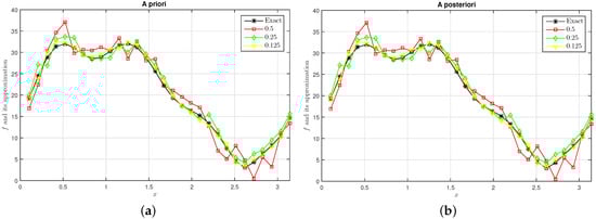
Figure 1. The exact approximation for a priori (a) and a posteriori (b).

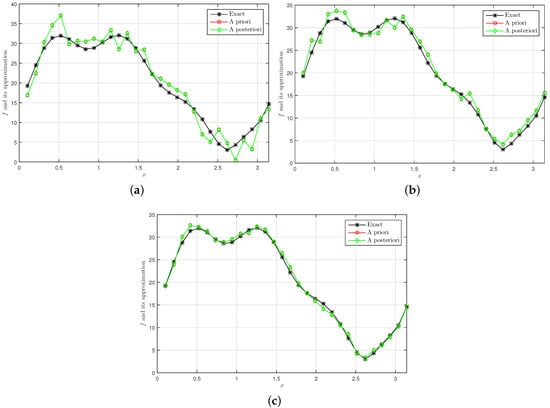
Figure 2. A priori and a posteriori when (a) $\delta =0.5$, (b) $\delta =0.25$ and (c) $\delta =0.125$, respectively.

References

- Alharbia, F.M.; Baleanu, D.; Abdelhalim, E. Physical properties of the projectile motion using the conformable derivative. Chin. J. Phys. 2019, 58, 18–28. [Google Scholar] [CrossRef]
- Kilbas, A.A.; Marichev, O.I.; Samko, S.G. Fractional Integrals and Derivatives (Theory and Applications), 1st ed.; CRC Press: Boca Raton, FL, USA, 1993. [Google Scholar]
- Tuan, N.H.; Aghdam, Y.E.; Jafari, H.; Mesgarani, H. A novel numerical manner for two-dimensional space fractional diffusion equation arising in transport phenomena. Numer. Methods Part. Differ. Equ. 2021, 37, 1397–1406. [Google Scholar] [CrossRef]
- Luc, N.H.; Jafari, H.; Kumam, P.; Tuan, N.H. On an initial value problem for time fractional pseudo-parabolic equation with Caputo derivarive. Math. Methods Appl. Sci. 2022, 1–23. [Google Scholar] [CrossRef]
- Au, V.V.; Jafari, H.; Hammouch, Z.; Tuan, N.H. On a final value problem for a nonlinear fractional pseudo-parabolic equation. Electron. Res. Arch. 2021, 29, 1709–1734. [Google Scholar]
- Can, N.H.; Jafari, H.; Ncube, M.N. Fractional calculus in data fitting. Alex. Eng. J. 2020, 59, 3269–3274. [Google Scholar] [CrossRef]
- Tuan, N.H.; Nemati, S.; Ganji, R.M.; Jafari, H. Numerical solution of multi-variable order fractional integro-differential equations using the Bernstein polynomials. Eng. Comput. 2022, 38, 139–147. [Google Scholar] [CrossRef]
- Han, Y.; Xiong, X.; Xue, X. A fractional Landweber method for solving backward timefractional diffusion problem. Comput. Math. Appl. 2019, 78, 81–91. [Google Scholar] [CrossRef]
- Yang, S.; Xiong, X.; Han, Y. A modified fractional Landweber method for a backward problem for the inhomogeneous time-fractional diffusion equation in a cylinder. Int. J. Comput. Math. 2020, 97, 2375–2393. [Google Scholar] [CrossRef]
- Huynh, L.H.; Zhou, Y.; O’Regan, D.; Tuan, N.H. Fractional Landweber method for an initial inverse problem for time-fractional wave equations. Appl. Anal. 2021, 100, 860–878. [Google Scholar] [CrossRef]
- Chung, W.S. Fractional Newton mechanics with conformable fractional derivative. J. Comput. Appl. Math. 2015, 290, 150–158. [Google Scholar] [CrossRef]
- Morales-Delgado, V.F.; Gómez-Aguilar, J.F.; Escobar-Jiménez, R.F.; Taneco-Hernández, M.A. Fractional conformable derivatives of Liouville-Caputo type with low-fractionality. Phys. A Stat. Mech. Appl. 2018, 503, 424–438. [Google Scholar] [CrossRef]
- He, S.; Sun, K.; Mei, X.; Yan, B.; Xu, S. Numerical analysis of a fractional-order chaotic system based on conformable fractional-order derivative. Eur. Phys. J. Plus 2017, 132, 36. [Google Scholar] [CrossRef]
- Hama, M.F.; Rasul, R.R.Q.; Hammouch, Z.; Rasul, K.A.H.; Danane, J. Analysis of a stochastic SEIS epidemic model with the standard Brownian motion and Lévy jump. Results Phys. 2022, 37, 105477. [Google Scholar] [CrossRef]
- Hammouch, Z.; Rasul, R.Q.R.; Ouakka, A.; Elazzouzi, A. Mathematical analysis and numerical simulation of the Ebola epidemic disease in the sense of conformable derivative. Chaos Solitons Fractals 2022, 158, 112006. [Google Scholar] [CrossRef]
- Karthikeyan, K.; Murugapandian, G.S.; Hammouch, Z. On mild solutions of fractional impulsive differential systems of Sobolev type with fractional nonlocal conditions. Math. Sci. 2022, 36, 37. [Google Scholar] [CrossRef]
- Hamou, A.A.; Azroul, E.H.; Hammouch, Z.; Alaoui, A.L. A monotone iterative technique combined to finite element method for solving reaction-diffusion problems pertaining to non-integer derivative. Eng. Comput. 2022, 36, 105. [Google Scholar] [CrossRef]
- Gürbüz, M.; Akdemir, A.O.; Dokuyucu, M.A. Novel Approaches for Differentiable Convex Functions via the Proportional Caputo-Hybrid Operators. Fractal Fract. 2022, 6, 258. [Google Scholar] [CrossRef]
- Avcı, A.M.; Akdemir, A.O.; Set, E. On New Integral Inequalities via Geometric-Arithmetic Convex Functions with Applications. Sahand Commun. Math. Anal. 2022. [Google Scholar] [CrossRef]
- Butt, S.I.; Akdemir, A.O.; Agarwal, P.; Baleanu, D. Non-conformable integral inequalities of chebyshev-polya-szeg o type. J. Math. Inequalities 2021, 4, 1391–1400. [Google Scholar] [CrossRef]
- Kavurmacı Önalan, H.; Akdemir, A.O.; Avcı Ardıç, M.; Baleanu, D. On new general versions of Hermite–Hadamard type integral inequalities via fractional integral operators with Mittag-Leffler kernel. J. Inequalities Appl. 2021, 1, 186. [Google Scholar] [CrossRef]
- Khalil, R.; Al Horani, M.; Yousef, A.; Sababheh, M. A new definition of fractional derivative. J. Comput. Appl. Math. 2014, 264, 65–70. [Google Scholar] [CrossRef]
- Abdelhakim, A.A.; Machado, J.A.T. A critical analysis of the conformable derivative. Nonlinear Dyn. 2019, 95, 3063–3073. [Google Scholar] [CrossRef]
- Abdeljawad, T. On conformable fractional calculus. J. Comput. Appl. Math. 2015, 279, 57–66. [Google Scholar] [CrossRef]
- Tuan, N.H.; Huynh, L.N.; Ngoc, T.B.; Zhou, Y. On a backward problem for nonlinear fractional diffusion equations. Appl. Math. Lett. 2019, 92, 76–84. [Google Scholar] [CrossRef]
- Ikehata, R.; Suzuki, T. Stable and unstable sets for evolution equations of parabolic and hyperbolic type. Hiroshima Math. J. 1996, 26, 475–491. [Google Scholar] [CrossRef]
- Quittner, P.; Souplet, P. Superlinear Parabolic Problems, Blow-Up, Global Existence and Steady States; Birkhäuser Advanced Texts; Birkhäuser Basel: Basel, Switzerland, 2007. [Google Scholar]
- Liu, Y.; Xu, R.; Yu, T. Global existence, nonexistence and asymptotic behavior of solutions for the Cauchy problem of semilinear heat equations. Nonlinear Anal. 2008, 68, 3332–3348. [Google Scholar] [CrossRef]
- Can, N.H.; Kumar, D.; Vo Viet, T.; Nguyen, A.T. On time fractional pseudo-parabolic equations with non-local in time condition. Math. Methods Appl. Sci. 2021. [Google Scholar] [CrossRef]
- Nguyen, A.T.; Hammouch, Z.; Karapinar, E.; Tuan, N.H. On a nonlocal problem for a Caputo time-fractional pseudoparabolic equation. Math. Methods Appl. Sci. 2021, 44, 14791–14806. [Google Scholar] [CrossRef]
- Nguyen, H.T.; Vo, V.A.; Runzhang, X. Semilinear Caputo time-fractional pseudo-parabolic equations. Commun. Pure Appl. Anal. 2021, 20, 583–621. [Google Scholar] [CrossRef]
- Nguyen, H.T.; Le, D.L.; Nguyen, V.T. Regularized solution of an inverse source problem for a time fractional diffusion equation. Appl. Math. Model. 2016, 40, 8244–8264. [Google Scholar] [CrossRef]
- Tuan, N.H.; Zhou, Y.; Long, L.D.; Can, N.H. Identifying inverse source for fractional diffusion equation with Reimann-Liouville derivetive. Comput. Appl. Math. 2020, 39, 75. [Google Scholar] [CrossRef]
- Long, L.D.; Luc, N.H.; Zhou, Y.; Nguyen, A.C. Identification of Source term for the time-fractional duffusion-wave equation by Fractional Tikhonov method. Mathematics 2019, 7, 934. [Google Scholar] [CrossRef] [Green Version]
- Long, L.D.; Zhou, Y.; Thanh Binh, T.; Can, N. A Mollification Regularization Method for the Inverse Source Problem for a Time Fractional Diffusion Equation. Mathematics 2019, 7, 1048. [Google Scholar] [CrossRef] [Green Version]
- Wei, T.; Li, X.L.; Li, Y.S. An inverse time-dependent source problem for a time-fractional diffusion equation. Inverse Probl. 2016, 32, 8. [Google Scholar] [CrossRef]
- Wang, J.G.; Zhou, Y.B.; Wei, T. Two regularization methods to identify a space-dependent source for the time-fractional diffusion equation. Appl. Numer. Math. 2013, 68, 39–57. [Google Scholar] [CrossRef]
- Tuan, N.H. On some inverse problem for bi-parabolic equation with observed data in Lp spaces. Opuscula Math. 2022, 42, 305–335. [Google Scholar] [CrossRef]
- Can, N.H.; Luc, N.H.; Baleanu, D.; Yong, Z.; Long, L.D. Inverse source problem for time fractional diffusion equation with Mittag-Leffler kernel. Adv. Differ. Equ. 2020, 2020, 210. [Google Scholar] [CrossRef]
- Tuan, N.H.; Caraballo, T. On initial and terminal value problems for fractional nonclassical diffusion equations. Proc. Am. Math. Soc. 2021, 149, 143–161. [Google Scholar] [CrossRef]
- Jaiswal, A.; Bahuguna, D. Semilinear Conformable Fractional Differential Equations in Banach Spaces. Differ. Equ. Dyn. Syst. 2019, 27, 313–325. [Google Scholar] [CrossRef]
- Li, M.; Wang, J.R.; O’Regan, D. Existence and Ulam’s stability for conformable fractional differential equations with constant coefficients. Bull. Malays. Math. Sci. Soc. 2019, 42, 1791–1812. [Google Scholar] [CrossRef]
Publisher’s Note: MDPI stays neutral with regard to jurisdictional claims in published maps and institutional affiliations. |
© 2022 by the authors. Licensee MDPI, Basel, Switzerland. This article is an open access article distributed under the terms and conditions of the Creative Commons Attribution (CC BY) license (https://creativecommons.org/licenses/by/4.0/).