Distance Antimagic Product Graphs

Abstract

A distance antimagic graph is a graph G admitting a bijection $f:V(G)\to \{1,2,\dots ,|V(G)\left|\right\}$ such that for two distinct vertices x and y, $\omega (x)\ne \omega (y)$, where $\omega (x)={\sum }_{y\in N(x)}f(y)$, for $N(x)$ the open neighborhood of x. It was conjectured that a graph G is distance antimagic if and only if G contains no two vertices with the same open neighborhood. In this paper, we study several distance antimagic product graphs. The products under consideration are the three fundamental graph products (Cartesian, strong, direct), the lexicographic product, and the corona product. We investigate the consequence of the non-commutative (or sometimes called non-symmetric) property of the last two products to the antimagicness of the product graphs.

1. Introduction

Let $G=G(V,E)$ be a finite, simple, and undirected graph of order n.

In 1994, Vilfred introduced distance magic labeling in his Ph.D. thesis [1]. A distance magic labeling of a graph G is a bijection $f:V(G)\to \{1,2,\dots ,n\}$ such that at any vertex x, the weight of x, $\omega (x)={\sum }_{y\in N(x)}f(y)$ is constant, where $N(x)$ is the open neighborhood of x, i.e., the set of vertices adjacent to x. In 2013, the notion of distance antimagic labeling of a graph G was then introduced by Kamatchi and Arumugam [2]. A bijection $f:V(G)\to \{1,2,\dots ,n\}$ is called a distance antimagic labeling of graph G if for two distinct vertices x and y their weights are also distinct, i.e., $\omega (x)\ne \omega (y)$. A graph admitting a distance antimagic labeling is called a distance antimagic graph. In the same paper, Kamatchi and Arumugam conjectured the following.

Conjecture 1

([2]). A graph G is distance antimagic if and only if G does not have two vertices with the same open neighborhood.

Some graphs supporting the truth of Conjecture 1 are, among others, the path $P_n$, the cycle $C_n$ ($n\ne 4$), the wheel $W_n$ ($n\ne 4$) [2], and the hypercube $Q_n$ ($n\ge 3$) [3]. In 2016, Llado and Miller [4] utilized Combinatorial Nullstellensatz to prove that a tree with l leaves and $2l$ vertices is distance antimagic.

In 2017, Arumugam et al. [5] and Bensmail et al. [6] introduced a weaker notion of antimagic labeling, called local antimagic labeling, where only adjacent vertices must be distinguished. It was conjectured in both articles that any connected graph other than $K_2$ admits local antimagic labeling. This conjecture has been completely settled by Haslegrave [7] using the probabilistic method.

A generalization of the distance antimagic labeling was proposed in [8]. Suppose that $D\subseteq \{0,1,\dots ,diam(G)\}$ is a set of distances and $N_D(x)=\left\{y\right|d(x,y)=d,d\in D\}$ is the D-neighborhood of the vertex x. A D-antimagic labeling of a graph G is a bijection $f:V(G)\to \{1,\dots ,n\}$ such that the weight ${\omega }_D(x)={\sum }_{y\in N_D(x)}f(y)$ is distinct for each vertex x. It was conjectured that a graph admits a D-antimagic labeling if and only if it does not contain two vertices having the same D-neighborhood.

In the rest of the paper, we shall prove that Conjecture 1 is true for some product graphs. We consider the three fundamental graph products (Cartesian, strong, and direct products), the lexicographic product, and the corona product. First, Section 2 provides definitions and notations of the graph products under consideration. Next, Section 3 considers distance antimagic graphs obtained from Cartesian, strong, and direct products. Then, in Section 4, we present distance antimagic lexicographic product graphs. Finally, in Section 5, we present distance antimagic corona product graphs. Since the corona product is not commutative (or sometimes called not symmetric) in general, we shall investigate the consequence of that property to the antimagicness of the product graphs.

2. Graph Products: Definition and Notation

This section presents definitions of the graph products considered in this paper. We start with the three fundamental graph products: Cartesian, strong, and direct. In all three products, the product of graphs G and H is another graph whose vertex set is the Cartesian product of sets $V(G)\times V(H)$. However, each product has different rules for adjacencies. All notations of the fundamental graph products are taken from [9].

Definition 1.

The Cartesian product of G and H, denoted by $G\square H$, is the graph with $V(G\square H)=V(G)\times V(H)$ and two vertices $(u,u^{\prime })$ and $(v,v^{\prime })$ are adjacent if and only if either

1. 

$u=v$ and $u^{\prime }$ is adjacent to $v^{\prime }$ in H, or

2. 

$u^{\prime }=v^{\prime }$and u is adjacent to v in G.

Definition 2.

The direct product of G and H, denoted by $G\times H$, is the graph with $V(G\times H)=V(G)\times V(H)$ and the two vertices $(u,u^{\prime })$ and $(v,v^{\prime })$ are adjacent if and only if u is adjacent to v and $u^{\prime }$ is adjacent to $v^{\prime }$.

Definition 3.

The strong product of G and H, denoted by $G⊠H$, is the graph with $V(G⊠H)=V(G)\times V(H)$, and the two vertices $(u,u^{\prime })$ and $(v,v^{\prime })$ are adjacent if and only if either

1. 

u is adjacent to v, and $u^{\prime }$ is adjacent to $v^{\prime }$, or

2. 

$u=v$ and $u^{\prime }$ is adjacent to $v^{\prime }$ in H, or

3. 

$u^{\prime }=v^{\prime }$ and u is adjacent to v in G.

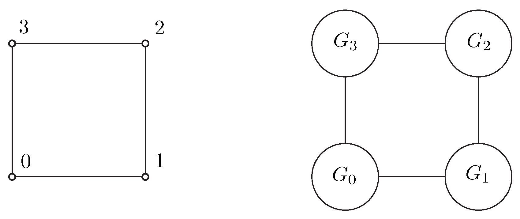
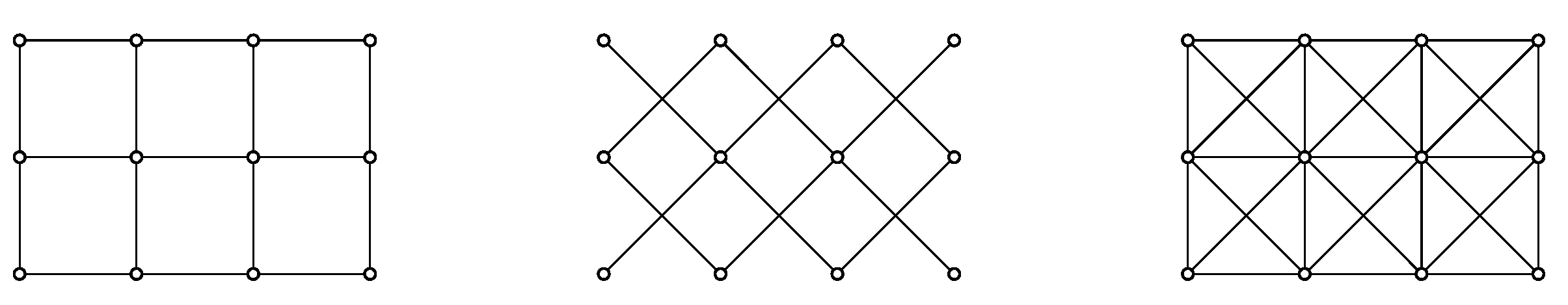
Note that $G\square H$ and $G\times H$ are subgraphs of $G⊠H$. The Cartesian, the direct, and the strong products are both commutative (or sometimes called symmetric) and associative. Thus we can omit parentheses when dealing with products with more than two factors. Refer to Figure 1 for examples of the three fundamental graph products.

The next product, the lexicographic product, although associative, is not commutative [9]. An example for the lexicographic product is presented in Figure 2.

Definition 4.

The lexicographic product of graphs G and H, denoted by $G\circ H$, is a graph with $V(G\circ H)=V(G)\times V(H)$ and the two vertices $(u,u^{\prime })$ and $(v,v^{\prime })$ are adjacent if and only if either

1. 

$u=v$ and $u^{\prime }$ is adjacent to $v^{\prime }$ in H, or

2. 

u and v are adjacent in G.

The final graph product under consideration is the corona product, which is generally not commutative and is never associative. For examples of the corona product, refer to Figure 3.

Definition 5

([10]). The corona product of G and H, denoted by $G\odot H$, is the graph obtained by taking a copy of G and $|V(G)|$ copies of H and joining the i-th vertex of G to every vertex in the i-th copy of H.

In the upcoming sections, we frequently use the following property of graphs.

Definition 6.

A graph G is called monotone if there exists a vertex labeling λ, i.e., a bijection $\lambda :V(G)\to \{1,2,\dots ,n\}$, such that $\lambda (u)<\lambda (v)$ implies $\omega (u)\le \omega (v)$ for every pair of distinct vertices $u,v$ in G.

It is obvious that every distance magic graph is monotone. An example of a non-distance magic but the monotone graph is the even path $P_{2k}=v_1{v}_2\dots v_{2k-1}{v}_{2k}$, where vertices $v_1,v_2,\dots ,v_k$ are labeled with consecutive odd integers and $v_{2k},v_{2k-1},\dots ,v_{k+1}$ are labeled with consecutive even integers. On the other hand, every complete graph of order at least 2 is non-monotone.

3. Distance Antimagic Graphs Obtained from Fundamental Graph Products

This section studies the distance antimagicness of graphs produced by three fundamental graph products: the Cartesian product, the strong product, and the direct product.

In [2], Kamatchi and Arumugam posed whether the Cartesian product $G\square K_2$ is distance antimagic. A partial positive answer was given in [11], where it was proven that $C_n\square K_2$ is distance antimagic. In the next two theorems, we answer the previous question for the cases of $G\in \{P_n,K_{n,n}\}$.

Theorem 1.

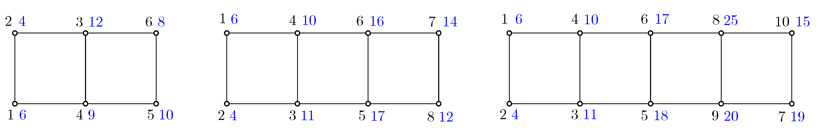
$P_n\square K_2$ is distance antimagic if and only if $n\ne 2$.

Proof. 

It is obvious that $P_2\square K_2\simeq C_4$ is not distance antimagic. For the remaining values of n, we define a vertex labeling $\lambda$.

Let $V(K_2\square P_n)=\left\{(x_i,y_j)\right|x_i\in K_2,y_j\in P_n\}$ and use the following notations ${\lambda }_{ij}=\lambda (x_i,y_j)$ and ${\omega }_{ij}=\omega (x_i,y_j)$.

Case 1. For $n\equiv 0mod3$:

$${\lambda }_{1j}=\left\{\begin{array}{cc}2j-1\hfill & ,j\mathrm{odd}\hfill \\ 2j\hfill & ,j\mathrm{even}\hfill \end{array}\right.$$

$${\lambda }_{2j}=\left\{\begin{array}{cc}2j\hfill & ,j\mathrm{odd}\hfill \\ 2j-1\hfill & ,j\mathrm{even}.\hfill \end{array}\right.$$

The weights induced by the labeling as mentioned above are:

$${\omega }_{1j}=\left\{\begin{array}{cc}6j\hfill & ,1\le j\le n-1,j\mathrm{odd}\hfill \\ 6j-3\hfill & ,1\le j\le n-1,j\mathrm{even}\hfill \\ 4n-2\hfill & ,j=n\mathrm{odd}\hfill \\ 4n-4\hfill & ,j=n\mathrm{even}\hfill \end{array}\right.$$

$${\omega }_{2j}=\left\{\begin{array}{cc}4\hfill & ,j=1\hfill \\ 6j-3\hfill & ,2\le j\le n-1,j\mathrm{odd}\hfill \\ 6j\hfill & ,2\le j\le n-1,j\mathrm{even}\hfill \\ 4n-4\hfill & ,j=n\mathrm{odd}\hfill \\ 4n-2\hfill & ,j=n\mathrm{even}\hfill \end{array}\right.$$

Case 2. For $n\equiv 1mod3$:

$${\lambda }_{1j}=\left\{\begin{array}{cc}2j-1\hfill & ,2\le j\le n-1\hfill \\ 2j\hfill & ,j=1,n\hfill \end{array}\right.$$

$${\lambda }_{2j}=\left\{\begin{array}{cc}2j\hfill & ,2\le j\le n-1\hfill \\ 2j-1\hfill & ,j=1,n,\hfill \end{array}\right.$$

and thus

$${\omega }_{1j}=\left\{\begin{array}{cc}4\hfill & ,j=1\hfill \\ 6j-2\hfill & ,3\le j\le n-2\hfill \\ 6j-1\hfill & ,j=2,n-1\hfill \\ 4n-4\hfill & ,j=n\hfill \end{array}\right.$$

$${\omega }_{2j}=\left\{\begin{array}{cc}6\hfill & ,j=1\hfill \\ 6j-1\hfill & ,3\le j\le n-2\hfill \\ 6j-2\hfill & ,j=2,n-1\hfill \\ 4n-2\hfill & ,j=n\hfill \end{array}\right.$$

Case 3. For $n\equiv 2mod3,n\ne 2$:

$${\lambda }_{1j}=\left\{\begin{array}{cc}2\hfill & ,j=1\hfill \\ 2j-1\hfill & ,2\le j\le n-2\hfill \\ 2n-1\hfill & ,j=n-1\hfill \\ 2n-3\hfill & ,j=n\hfill \end{array}\right.$$

$${\lambda }_{2j}=\left\{\begin{array}{cc}1\hfill & ,j=1\hfill \\ 2j\hfill & ,j\ge 2,\hfill \end{array}\right.$$

which lead to

$${\omega }_{1j}=\left\{\begin{array}{cc}4\hfill & ,j=1\hfill \\ 11\hfill & ,j=2\hfill \\ 6j-2\hfill & ,3\le j\le n-3\hfill \\ 6j\hfill & ,j=n-2\hfill \\ 6j-4\hfill & ,j=n-1\hfill \\ 6n-1\hfill & ,j=n\hfill \end{array}\right.$$

$${\omega }_{2j}=\left\{\begin{array}{cc}6\hfill & ,j=1\hfill \\ 10\hfill & ,j=2\hfill \\ 6j-1\hfill & ,3\le j\le n-2\hfill \\ 6j+1\hfill & ,j=n-1\hfill \\ 4n-5\hfill & ,j=n.\hfill \end{array}\right.$$

In all three cases, the weight of each vertex is distinct. Examples of the labelings for $P_n\square K_2,n=3,4,5$ can be seen in Figure 4. □

Theorem 2.

$K_{n,n}\square K_2$ is distance antimagic if and only if $n\ne 1$.

Proof. 

Suppose that X and Y are the natural bipartition sets of $V(K_{n,n})$. Let ${\lambda }^{\prime }$ be a vertex labeling of $K_{n,n}$ where the vertices in X are labeled with $1,2,\dots ,n$ and those in Y are labeled with $n+1,n+2,\dots ,2n$. Define a labeling $\lambda$ for $K_{n,n}\square K_2$ by $\lambda (v,1)={\lambda }^{\prime }(v)$ and $\lambda (v,2)={\lambda }^{\prime }(v)+2n$.

We denote it by $K_1=\left\{(x,1)\right|x\in X\},K_2=\left\{(y,1)\right|y\in Y\},K_3=\left\{(x,2)\right|x\in X\}$, and $K_4=\left\{(y,2)\right|y\in Y\}$ (see Figure 5). Let $k_a$ be the sum of all labels in $K_a$, which are $k_1=\left(\genfrac{}{}{0pt}{}{n+1}{2}\right),k_2=k_1+n^2,k_3=k_1+2n^2$, and $k_4=k_1+3n^2$. Then the vertex-weights in $K_{n,n}$ are

$$\omega (v)=\left\{\begin{array}{cc}{k}_2+\lambda (v)+2n\hfill & ,v\in K_1,\hfill \\ k_1+\lambda (v)+2n\hfill & ,v\in K_2,\hfill \\ k_4+\lambda (v)-2n\hfill & ,v\in K_3,\hfill \\ k_3+\lambda (v)-2n\hfill & ,v\in K_4.\hfill \end{array}\right.$$

Let u and v be two arbitrary vertices in $K_a$ and $K_b$, respectively. If $a=b$ then $\omega (u)-\omega (v)=\lambda (u)-\lambda (v)$, which is not zero. If $a\ne b$, it is easy to check that $\omega (u)-\omega (v)\ne 0$ by considering $1-n<\lambda (u)-\lambda (v)<n-1.$ □

In the next theorem, we change the factor $K_2$ into $K_3$ and study the antimagicness of $P_n\square K_3$.

Theorem 3.

For $n\ge 1$, $P_n\square K_3$ is distance antimagic.

Proof. 

Let $V(P_n\times K_3)=\left\{(x_i,y_j)\right|x_i\in V(P_n),y_j\in V(K_3)\}$. In the following four cases, we define a vertex labeling $\lambda$ and denote it by ${\lambda }_{ij}=\lambda (x_i,y_j)$ and ${\omega }_{ij}=\omega (x_i,y_j)$.

Case 1. For n even:

$${\lambda }_{1j}=\left\{\begin{array}{cc}3j-2\hfill & ,j\mathrm{odd}\hfill \\ 3j\hfill & ,j\mathrm{even}.\hfill \end{array}\right.$$

$${\lambda }_{2j}=3j-1,1\le j\le n.$$

$${\lambda }_{3j}=\left\{\begin{array}{cc}3j\hfill & ,j\le n-2,j\mathrm{odd}\hfill \\ 3j-2\hfill & ,j\le n-2,j\mathrm{even}\hfill \\ 3n-2\hfill & ,j=n-1\hfill \\ 3n-3\hfill & ,j=n.\hfill \end{array}\right.$$

Therefore, for $n=2$, ${\omega }_{11}=12,{\omega }_{12}=9,{\omega }_{21}=10,{\omega }_{22}=11,{\omega }_{31}=6$, and ${\omega }_{32}=15$. For $n\ge 4$,

$${\omega }_{1j}=\left\{\begin{array}{cc}11\hfill & ,j=1\hfill \\ 12j-1\hfill & ,2\le j\le n-2,j\mathrm{odd}\hfill \\ 12j-7\hfill & ,2\le j\le n-2,j\mathrm{even}\hfill \\ 12n-13\hfill & ,j=n-1\hfill \\ 9n-8\hfill & ,j=n\hfill \end{array}\right.$$

$${\omega }_{2j}=\left\{\begin{array}{cc}9\hfill & ,j=1\hfill \\ 12j-4\hfill & ,2\le j\le n-2\hfill \\ 12n-15\hfill & ,j=n-1\hfill \\ 9n-7\hfill & ,j=n\hfill \end{array}\right.$$

$${\omega }_{3j}=\left\{\begin{array}{cc}7\hfill & ,j=1\hfill \\ 12j-7\hfill & ,2\le j\le n-3,j\mathrm{odd}\hfill \\ 12j-1\hfill & ,2\le j\le n-3,j\mathrm{even}\hfill \\ 12n-24\hfill & ,j=n-2\hfill \\ 12n-20\hfill & ,j=n-1\hfill \\ 9n-3\hfill & ,j=n.\hfill \end{array}\right.$$

Case 2. For $n\equiv 1mod4,n\ne 5$:

$${\lambda }_{1j}=\left\{\begin{array}{cc}3j-2\hfill & ,j\mathrm{odd}\hfill \\ 3j\hfill & ,j\mathrm{even}\hfill \end{array}\right.$$

$${\lambda }_{2j}=3j-1,1\le j\le n$$

$${\lambda }_{3j}=\left\{\begin{array}{cc}3j\hfill & ,j\le n-2,j\mathrm{odd}\hfill \\ 3j-2\hfill & ,j\le n-2,j\mathrm{even}\hfill \\ 3n\hfill & ,j=n-1\hfill \\ 3n-5\hfill & ,j=n,\hfill \end{array}\right.$$

and so

$${\omega }_{1j}=\left\{\begin{array}{cc}11\hfill & ,j=1\hfill \\ 12j-1\hfill & ,2\le j\le n-2,j\mathrm{odd}\hfill \\ 12j-7\hfill & ,2\le j\le n-2,j\mathrm{even}\hfill \\ 12n-14\hfill & ,j=n-1\hfill \\ 9n-9\hfill & ,j=n\hfill \end{array}\right.$$

$${\omega }_{2j}=\left\{\begin{array}{cc}9\hfill & ,j=1\hfill \\ 12j-4\hfill & ,2\le j\le n-2\hfill \\ 12n-10\hfill & ,j=n-1\hfill \\ 9n-11\hfill & ,j=n\hfill \end{array}\right.$$

$${\omega }_{3j}=\left\{\begin{array}{cc}7\hfill & ,j=1\hfill \\ 12j-7\hfill & ,2\le j\le n-3,j\mathrm{odd}\hfill \\ 12j-1\hfill & ,2\le j\le n-3,j\mathrm{even}\hfill \\ 12n-26\hfill & ,j=n-2\hfill \\ 12n-18\hfill & ,j=n-1\hfill \\ 9n-3\hfill & ,j=n.\hfill \end{array}\right.$$

Case 3. For $n=5$ or $n\equiv 3mod4,n\ne 3$:

$${\lambda }_{1j}=\left\{\begin{array}{cc}3j-2\hfill & ,j\mathrm{odd}\hfill \\ 3j\hfill & ,j\mathrm{even}\hfill \end{array}\right.$$

$${\lambda }_{2j}=\left\{\begin{array}{cc}3n\hfill & ,j=1\hfill \\ 3j-1\hfill & ,j\ge 2\hfill \end{array}\right.$$

$${\lambda }_{3j}=\left\{\begin{array}{cc}3j\hfill & ,j\mathrm{odd}\hfill \\ 3j-2\hfill & ,j\mathrm{even}\hfill \\ 2\hfill & ,j=n.\hfill \end{array}\right.$$

Thereforem

$${\omega }_{1j}=\left\{\begin{array}{cc}3n+9\hfill & ,j=1\hfill \\ 12j-1\hfill & ,2\le j\le n-1,j\mathrm{odd}\hfill \\ 12j-7\hfill & ,2\le j\le n-1,j\mathrm{even}\hfill \\ 6n-2\hfill & ,j=n\hfill \end{array}\right.$$

$${\omega }_{2j}=\left\{\begin{array}{cc}9\hfill & ,j=1\hfill \\ 3n+18\hfill & ,j=2\hfill \\ 12j-4\hfill & ,2\le j\le n-1\hfill \\ 6n-4\hfill & ,j=n\hfill \end{array}\right.$$

$${\omega }_{3j}=\left\{\begin{array}{cc}3n+5\hfill & ,j=1\hfill \\ 12j-7\hfill & ,2\le j\le n-2,j\mathrm{odd}\hfill \\ 12j-1\hfill & ,2\le j\le n-2,j\mathrm{even}\hfill \\ 9n-11\hfill & ,j=n-1\hfill \\ 9n-8\hfill & ,j=n.\hfill \end{array}\right.$$

Case 4. For $n=3$, define a vertex labeling ${\lambda }_{11}=1,{\lambda }_{12}=4,{\lambda }_{13}=3,{\lambda }_{21}=8,{\lambda }_{22}=7,$${\lambda }_{23}=5,{\lambda }_{31}=9,{\lambda }_{32}=2,{\lambda }_{33}=6$. Thus we obtain the following weights ${\omega }_{11}=21,$${\omega }_{12}=13,{\omega }_{13}=15,{\omega }_{21}=17,{\omega }_{22}=19,{\omega }_{23}=16,{\omega }_{31}=11,{\omega }_{32}=26,{\omega }_{33}=10$.

It is clear that the weights of the vertices are different in all cases. Examples of the labeling for $P_n\square K_3,n=6,7,9$ can be seen in Figure 6. □

In [12], it was proven that for any odd integer $n\ge 3$, $C_n\square K_3$ is distance antimagic. The same paper also asked whether $C_n\square K_3$ is distance antimagic when n is even. We then ask a more general question as in the following.

Problem 1.

Is $G\square K_3$ distance antimagic?

Our result is for distance magic instead of distance antimagic for the direct product.

Theorem 4.

Let G and H be regular distance magic graphs, then $G\times H$ is also distance magic.

Proof. 

Let ${\lambda }_G$ and ${\lambda }_H$ be distance magic labeling of G and H, respectively. Assume that G is on n vertices, $r_G$ and $r_H$ are the degree of vertices in G and H, respectively.

Define a labeling $\lambda$ for $G\times H$ as follows.

$$\lambda (u,v)={\lambda }_G(u)+({\lambda }_H(v)-1)n.$$

Then, we obtain the following vertex-weight for any vertex $(u,v)$.

$$\begin{array}{cc}\hfill \omega (u,v)& =\sum _{u^{\prime }\in N(u)}\sum _{v^{\prime }\in N(v)}\lambda (u^{\prime },v^{\prime })\hfill \\ \hfill & =\sum _{u^{\prime }\in N(u)}\sum _{v^{\prime }\in N(v)}({\lambda }_G(u^{\prime })+{\lambda }_H(v^{\prime })n-n)\hfill \\ \hfill & =r_H\sum _{u^{\prime }\in N(u)}{\lambda }_G(u^{\prime })+r_G\sum _{v^{\prime }\in N(v)}{\lambda }_H(v^{\prime })n-r_G{r}_{H}n\hfill \\ \hfill & =r_H{\omega }_G(u)+r_G{\omega }_H(v)-r_G{r}_{H}n.\hfill \end{array}$$

Since $r_H,{\omega }_G,r_G,{\omega }_H,$ and n are constant, then $\omega (u,v)$ is constant for every vertex $(u,v).$ □

We conclude this section by presenting some sufficient conditions for the strong product $G⊠H$ to be distance antimagic.

Theorem 5.

Let G be $r_G$-regular and H be $r_H$-regular, with $r_G\ge r_H$. If G is distance magic and H is monotone, then $G⊠H$ is distance antimagic.

Proof. 

Let ${\lambda }_G$ be a distance magic labeling of G with weigh ${\omega }_G$, and n be the order of G. Let ${\lambda }_H$ be a monotone labeling of H with weight ${\omega }_H$.

Define a labeling $\lambda$ for $G⊠H$ as $\lambda (u,v)={\lambda }_G(u)+({\lambda }_H(v)-1)n$. Thus for any vertex $(u,v)$, we obtain the following vertex-weight.

$$\begin{array}{cc}\hfill \omega (u,v)=& \sum _{u^{\prime }\in N(u)}\sum _{v^{\prime }\in N(v)}\lambda (u^{\prime },v^{\prime })+\sum _{u^{\prime }\in N(u)}\lambda (u^{\prime },v^{\prime })+\sum _{v^{\prime }\in N(v)}\lambda (u^{\prime },v^{\prime })\hfill \\ \hfill =& ({\omega }_G(u)+({\lambda }_H(v)-1)n)+\sum _{v^{\prime }\in N(v)}({\omega }_G(u)+r_G({\lambda }_H(v^{\prime })-1)n)\hfill \\ \hfill & +\sum _{v^{\prime }\in N(v)}({\lambda }_G(u)+({\lambda }_H(v^{\prime })-1)n)\hfill \\ \hfill =& ({\omega }_G(u)+{\lambda }_H(v)r_{G}n-r_{G}n)+(r_H{\omega }_G(u)+{\omega }_H(v)r_{G}n-r_H{r}_{G}n)\hfill \\ \hfill & +(r_H{\lambda }_G(u)+{\omega }_H(v)n-r_{H}n).\hfill \end{array}$$

Let $(u_1,v_1)$ and $(u_2,v_2)$ be two distinct vertices in $G⊠H$, with ${\lambda }_H(v_1)>{\lambda }_H(v_2)$. Then

$$\begin{array}{cc}\hfill \omega (u_1,v_1)-\omega (u_2,v_2)=& {\lambda }_H(v_1)r_{G}n+{\omega }_H(v_1)r_{G}n+r_H{\lambda }_G(u_1)+{\omega }_H(v_1)n\hfill \\ \hfill & -{\lambda }_H(v_2)r_{G}n-{\omega }_H(v_2)r_{G}n-r_H{\lambda }_G(u_2)-{\omega }_H(v_2)n\hfill \\ \hfill \ge & r_{G}n+0+r_H(1-n)+0>0.\hfill \end{array}$$

□

In Theorem 5, H must be monotone for $G⊠H$ to be distance antimagic. In the following, we present an example of a non-monotone graph H, that is $n{P}_2$, where $G⊠H$ is distance antimagic.

Theorem 6.

If G is regular and distance magic, then $G⊠n{P}_2$ is distance antimagic.

Proof. 

Let ${\lambda }_P$ be a labeling of $n{P}_2$ with the vertex labeled i adjacent to the vertex labeled $i+1$ for $i=1,3,\dots ,2n-1$. Let m be the order of G, r be the degree of vertices in G, and ${\lambda }_G$ be a distance antimagic labeling of G.

Define a labeling $\lambda$ for $G⊠n{P}_2$ as

$$\lambda (u,v)={\lambda }_G(u)+({\lambda }_P(v)-1)m.$$

Suppose that $v^{\prime }$ is the neighbor of v in $P_2$, then,

$$\begin{array}{cc}\hfill \omega (u,v)& =\sum _{u^{\prime }\in N(u)}\sum _{v^{\prime }\in N(v)}\lambda (u^{\prime },v^{\prime })+\sum _{u^{\prime }\in N(u)}\lambda (u^{\prime },v^{\prime })+\sum _{v^{\prime }\in N(v)}\lambda (u^{\prime },v^{\prime })\hfill \\ \hfill & =({\omega }_G(u)+({\lambda }_P(v)-1)rm)+({\omega }_G(u)+({\lambda }_P(v^{\prime })-1)rm)+({\lambda }_G(u)+({\lambda }_P(v^{\prime })-1)m)\hfill \\ \hfill & =2{\omega }_G(u)+{\lambda }_G(u)-2rm+({\lambda }_P(v)-{\lambda }_P(v^{\prime }))rm+({\lambda }_P(v^{\prime })-1)m.\hfill \end{array}$$

Let $(u_1,v_1)$ and $(u_2,v_2)$ be two vertices in $V(G⊠n{P}_2)$ with ${\lambda }_P(v_1^{\prime })>{\lambda }_P(v_2^{\prime })$. Then,

$$\begin{array}{cc}\hfill \omega (u_1,v_1)-\omega (u_2,v_2)=& {\lambda }_G(u_1)-{\lambda }_G(u_2)+({\lambda }_P(v_1)+{\lambda }_P(v_1^{\prime })-{\lambda }_P(v_2)-{\lambda }_P(v_2^{\prime }))\hfill \\ \hfill & +({\lambda }_P(v_1^{\prime })-{\lambda }_P(v_2^{\prime }))m\hfill \\ \hfill \ge & 1-m+m>0.\hfill \end{array}$$

□

4. Distance Antimagic Graphs Obtained from the Lexicographic Product

This section studies distance antimagic labelings of graphs obtained from the lexicographic product. We start with two lemmas on the vertex-weight.

Lemma 1.

Let G be an r-regular graph on n vertices and let f be any vertex labeling of G. Then, for two vertices $u,v$ in G, ${\omega }_f(u)-{\omega }_f(v)+n^2-rn>0.$

Proof. 

$$\begin{array}{cc}\hfill 2{(n-r)}^2& >0\hfill \\ \hfill 2r^2+2n^2-4rn& >0\hfill \\ \hfill r+r^2-(2nr-r^2+r)+2n^2-2rn& >0\hfill \\ \hfill \frac{1+r}{2}r-\frac{n+n-r+1}{2}r+n^2-rn& >0.\hfill \end{array}$$

Since $\frac{1+r}{2}r\le \omega (v)\le \frac{n+n-r+1}{2}r$ for $v\in V(G)$,

$$\begin{array}{cc}\hfill \omega (u)-\omega (v)+n^2-rn& >0.\hfill \end{array}$$

□

Lemma 2.

Let G be an r-regular graph on n vertices and let f be any vertex labeling of G. Then, for two vertices $u,v$ in G, ${\omega }_f(u)-{\omega }_f(v)+rn>0$.

Proof. 

$$\begin{array}{cc}\hfill 2r^2& >0\hfill \\ \hfill r+r^2-(2nr-r^2+r)+2rn& >0\hfill \\ \hfill \frac{1+r}{2}r-\frac{n+n-r+1}{2}r+rn& >0.\hfill \end{array}$$

Since $\frac{1+r}{2}r\le \omega (v)\le \frac{n+n-r+1}{2}r$ for $v\in V(G)$, we have

$$\begin{array}{cc}\hfill \omega (u)-\omega (v)+rn& >0.\hfill \end{array}$$

□

Definition 7.

Let G be an r-regular distance antimagic graph of order n and H be a graph. Suppose ${\lambda }_G$ is a distance antimagic labeling of G and ${\lambda }_H:V(H)\to \{0,1,\dots |V(H)|-1\}$ is labeling of H. For $a\in V(H)$, let$G_a$be the subgraph of $H\circ G$ induced by $\{(a,v)|v\in V(G)\}$. Define a labeling λ for $H\circ G$ by $\lambda (a,v)={\lambda }_G(v)+{\lambda }_H(a)n$ for $(a,v)\in V(H\circ G)$.

An illustration for the notation of $G_a$ is given in Figure 7.

The following properties hold for the labeling of $\lambda$ in Definition 7.

Lemma 3.

Let $k_0=\left(\genfrac{}{}{0pt}{}{n+1}{0}\right)$. If $k_a$ is the sum of all labels in $G_a$, then $k_a=k_0+{\lambda }_H(a)n^2$ and $\omega (a,v)={\omega }_G(v)+{\lambda }_H(a)rn+d_H(a)k_0+{\omega }_H(a)n^2.$

Proof. 

$$\begin{array}{cc}\hfill \omega (a,v)& =\sum _{u\in N_G(v)}\lambda (a,u)+\sum _{b\in N_H(a)}{k}_b\hfill \\ \hfill & =(\sum _{u\in N_G(v)}{\lambda }_G(u)+{\lambda }_H(a)n)+(\sum _{b\in N_H(a)}{k}_0+{\lambda }_H(b)n^2)\hfill \\ \hfill & =({\omega }_G(v)+r{\lambda }_H(a)n)+(d_H(a)k_0+{\omega }_H(a)n^2).\hfill \end{array}$$

□

Definition 8.

Let H be a graph with $V(H)=\{a_1,a_2,...,a_n\}$. Define a vertex labeling ${\lambda }_H$ for H as follows.

$${\lambda }_H(a_i)=\left\{\begin{array}{cc}2i-2\hfill & ,i\le \frac{n+1}{2}\hfill \\ 2n-2i+1\hfill & ,i>\frac{n+1}{2}.\hfill \end{array}\right.$$

Now we are ready to prove our main result for the lexicographic product.

Theorem 7.

Let G and H be regular graphs. If G is distance antimagic and H is monotone, then $H\circ G$ is distance antimagic.

Proof. 

Label vertices in H by ${\lambda }_H$ in Definition 8. Let $(a,v_i)\in V(G_a)$ and $(b,v_j)\in V(G_b)$. If $a=b$, then $G_a$ is distance antimagic. If ${\lambda }_H(a)>{\lambda }_H(b)$, then

$$\begin{array}{cc}\hfill \omega (a,v_i)-\omega (b,v_j)& ={\omega }_G(v_i)-{\omega }_G(v_j)+({\lambda }_H(a)-{\lambda }_H(b))r_{G}n+(r_H-r_H)k_0\hfill \\ \hfill & +({\omega }_H(a)-{\omega }_H(b))n^2\hfill \\ \hfill & \ge {\omega }_G(v_i)-{\omega }_G(v_j)+rn.\hfill \end{array}$$

By Lemma 2, $\omega (a,v_i)-\omega (b,v_j)>0.$ □

If H is non-regular or non-monotone, in general, we do not know whether $H\circ G$ is distance antimagic or not. However, there exists a class of regular graphs H that is not monotone, where $H\circ G$ is distance antimagic, as presented in the next theorem.

Theorem 8.

If G is a regular distance antimagic graph, then $K_m\circ G$ is also distance antimagic.

Proof. 

Let r and n be the degree of a vertex in G and the order of G, respectively. Label the vertices in $H=K_m$ by ${\lambda }_H$ in Definition 8 and denote it by $S=\sum _{a\in V(K_m)}{\lambda }_H(a)$.

Choose two vertices $(a,v_i)\in V(G_a)$ and $(b,v_j)\in V(G_b)$. If $a=b$, $G_a$ is distance antimagic. If ${\lambda }_H(b)>{\lambda }_H(a)$,

$$\begin{array}{cc}\hfill \omega (a,v_i)-\omega (b,v_j)=& {\omega }_G(v_i)-{\omega }_G(v_j)+({\lambda }_H(a)-{\lambda }_H(b))rn\hfill \\ \hfill & +(d_H(a)-d_H(b))k_0+({\omega }_H(a)-{\omega }_H(b))n^2\hfill \\ \hfill =& {\omega }_G(v_i)-{\omega }_G(v_j)+({\lambda }_H(a)-{\lambda }_H(b))rn\hfill \\ \hfill & +0+(S-{\lambda }_H(a)-(S-{\lambda }_H(b)))n^2\hfill \\ \hfill =& {\omega }_G(v_i)-{\omega }_G(v_j)+({\lambda }_H(b)-{\lambda }_H(a))(n^2-rn)\hfill \\ \hfill \ge & {\omega }_G(v_i)-{\omega }_G(v_j)+n^2-rn.\hfill \end{array}$$

By Lemma 1, $\omega (a,v_i)-\omega (b,v_j)>0.$ □

In the next two theorems, we present examples of non-regular graphs H of which $H\circ G$ is distance antimagic.

Theorem 9.

If G is a regular distance antimagic graph, then $P_m\circ G$ is also distance antimagic.

Proof. 

Let n be the order of G and $P_m=(a_1{a}_2\dots a_m)$. For $m=2$, use Theorem 8. For $m=3$, define a labeling for $P_m$ by ${\lambda }_P(a_i)=i-1$. By Lemma 3, $\omega (1,v)={\omega }_G(v)+k_0+n^2,\omega (2,v)={\omega }_G(v)+2k_0+2n^2+rn,\omega (3,v)={\omega }_G(v)+k_0+n^2+2rn$. Then, due to Lemmas 1 and 2

$$\begin{array}{cc}\hfill \omega (2,v_i)-\omega (3,v_j)& ={\omega }_G(v_i)-{\omega }_G(v_j)+k_0+n^2-rn>0,\mathrm{and}\hfill \\ \hfill \omega (3,v_i)-\omega (1,v_j)& ={\omega }_G(v_i)-{\omega }_G(v_j)+rn>0.\hfill \end{array}$$

For $m\ge 4$, use the labeling ${\lambda }_H$ from Definition 8 for $P_m$ and the labeling $\lambda$ from Definition 7 for $P_m\circ G$. Let $(a,v_i)\in V{G}_a$ and $(b,v_j)\in V{G}_b$ where ${\lambda }_H(a)>{\lambda }_H(b)$.

$$\begin{array}{cc}\hfill \omega (a,v_i)-\omega (b,v_j)& ={\omega }_G(v_i)-{\omega }_G(v_j)+({\lambda }_H(a)-{\lambda }_H(b))rn\hfill \\ \hfill & +(d_H(a)-d_H(b))k_0+({\omega }_H(a)-{\omega }_H(b))n^2\hfill \\ \hfill & \ge {\omega }_G(v_i)-{\omega }_G(v_j)+rn.\hfill \end{array}$$

By Lemma 2, $\omega (a,v_i)-\omega (b,v_j)>0.$ □

Theorem 10.

If G is a regular distance antimagic graph, then $W_m\circ G$ is also distance antimagic.

Proof. 

For $m=3$ use Theorem 8. For $m\ge 4$, let $C_m=(v_1{v}_2...v_m{v}_1)$. Use a modification of ${\lambda }_H$ for $C_m$ from Definition 8 where ${\lambda }_H(v_{m+1})=m+1$. By this labeling, $W_n$ is monotone. Following the proof of Theorem 7 and considering $d(m+1)>d(i)$ for $i\le m$, we obtain that $W_m\circ G$ is distance antimagic. □

5. Distance Antimagic Graphs Obtained from the Corona Product

In [2], it was proven that $G\odot K_1$ is distance antimagic for arbitrary graph G. Thus, the following is an obvious consequence.

Corollary 1.

Let G be a graph. Then $G\odot \overline{K_n}$ is distance antimagic if and only if $n=1$.

Since the corona product is not commutative, we present sufficient conditions that $K_1\odot G$ is distance antimagic in the following two theorems.

Theorem 11.

If G is a distance antimagic graph of order n with $\Delta <n+\frac{1}{2}-\sqrt{2n+\frac{9}{4}}$, then $K_1\odot G$ is distance antimagic.

Proof. 

Let ${\lambda }_G$ be a distance antimagic labeling of G and $V(K_1\odot G)=V(G)\cup \left\{u\right\}$. Define a labeling for $K_1\odot G$ by $\lambda (v_i)={\lambda }_G(v_i)$ for $v_i\in V(G)$ and $\lambda (u)=n+1$. Then, $\omega (v_i)={\omega }_G(v_i)+(n+1)$ and $\omega (u)=\frac{1+n}{2}n$. Therefore, $\omega (v_i)\ne \omega (v_j)$ for distinct $v_i,v_j\in V(G)$.

For $\Delta <n+\frac{1}{2}-\sqrt{2n+\frac{9}{4}}$,

$$\begin{array}{cc}\hfill {\Delta }^2-(2n+1)\Delta +(n^2-n-2)& >0\hfill \\ \hfill 2n\Delta -{\Delta }^2+\Delta +2n+2& <n+n^2\hfill \\ \hfill \frac{n+n-\Delta +1}{2}\Delta +n+1& <\frac{1+n}{2}n.\hfill \end{array}$$

The left side of the last inequality is the maximum weight of any vertex in G. Hence, $\omega (v_i)\ne \omega (u),v_i\in V(G).$ □

Examples of graphs satisfying the condition of Theorem 11 are paths and cycles with $n\ge 5$, distance antimagic cubic graphs with $n\ge 7$, and distance antimagic bipartite graphs with $n\ge 8$. If the graph G is regular and distance antimagic instead, we could prove that $K_1\odot G$ is also distance antimagic.

Theorem 12.

If G is a distance antimagic regular graph, then $K_1\odot G$ is distance antimagic.

Proof. 

Suppose that $n,r,$ and ${\lambda }_G$ are the order, the degree, and a distance antimagic labeling of G, respectively. Define a labeling for $K_1\odot G$ by $\lambda (u)=1$ and $\lambda (v)={\lambda }_G(v)+1$ for $v\in V(G)$. Then, $\omega (v)={\omega }_G(v)+r+1$. Since u is adjacent to all vertices of G, then $\omega (u)>\omega (v)$ for all $v\in V(G).$ □

If we change the factor $K_1$ with $\overline{K_2}$, we obtain the following sufficient condition for $\overline{K_2}\odot G$ to be distance magic.

Theorem 13.

If G is r-regular distance antimagic graph on n vertices with $r<\frac{1}{2}(4n+5-\sqrt{12n^2+20n+33})$, then $\overline{K_2}\odot G$ is distance antimagic.

Proof. 

Let ${\lambda }_G$ be a distance antimagic labeling of G and $V(\overline{K_2}\odot G)=V(G_1)\cup V(G_2)\cup \{u_1,u_2\}$. Define a labeling for $\overline{K_2}\odot G$ by $\lambda (u_1)=2,\lambda (u_2)=1,\lambda (v_i)={\lambda }_G(v_i)+2$ for $v_i\in V(G_1)$ and $\lambda (v_i)={\lambda }_G(v_i)+2+n$ for $v_i\in V(G_2)$. By this labeling, the distinct vertex-weights of $G_1$ and $G_2$ are preserved. For $r<\frac{1}{2}(4n+5-\sqrt{12n^2+20n+33})$,

$$\begin{array}{cc}\hfill r^2-(4n+5)r+(n^2+5n-2)& >0\hfill \\ \hfill \frac{3+(n+2)}{2}n& >\frac{(2n+2)+(2n+2-r+1)}{2}r+1.\hfill \end{array}$$

The right side of the last inequality is the maximum vertex-weight in $V(G_2)$, while the left one is $\omega (u_1)$. Hence, $\omega (v_i)<\omega (v_j)<\omega (u_1)<\omega (u_2)$ for $v_i\in V(G_1),v_j\in V(G_2).$ □

Examples of graphs satisfying the sufficient condition of Theorem 13 are paths and cycles with $n\ge 5$ and distance antimagic cubic graphs with $n\ge 8$. However, in general, the antimagicness of $\overline{K_n}\odot G$ is still unknown and thus the following problem.

Problem 2.

For $n\ge 3$, is $\overline{K_n}\odot G$ distance antimagic?

In the last part of this section, we study the distance antimagicness of both $G\odot P_2$ and $P_2\odot G$. In addition, we can find other results for corona product graphs in [13], where it was proven that $C_4\odot C_n$ is distance antimagic for $n\ge 9$.

Theorem 14.

If G is r-regular distance antimagic graph on n vertices with $r<\frac{1}{2}(4n+5-\sqrt{12n^2+20n+25})$, then $P_2\odot G$ is distance antimagic.

Proof. 

The proof is similar to that of Theorem 13, by substituting $\omega (u_1)$ with $\frac{3+(n+2)}{2}n+1.$ □

Theorem 15.

If G is a monotone graph with a minimum degree of at least 3, then $G\odot P_2$ is distance antimagic.

Proof. 

Let $|V(G)|=n$. Denote $P_{2,v}$ as subgraph of $G\odot P_2$ induced by $\{(v,1),(v,2)\}$. Define a labeling for $G\odot P_2$ by,

$$\begin{array}{cc}\hfill \lambda (v,1)& =2{\lambda }_G(v)-1\hfill \\ \hfill \lambda (v,2)& =2{\lambda }_G(v)\hfill \\ \hfill \lambda (v)& ={\lambda }_G(v)+2n.\hfill \end{array}$$

Thus,

$$\begin{array}{cc}\hfill \omega (v,1)& =3{\lambda }_G(v)+2n\hfill \\ \hfill \omega (v,2)& =3{\lambda }_G(v)+2n-1\hfill \\ \hfill \omega (v)& ={\omega }_G(v)+d_G(v)·2n+4{\lambda }_G(v)-1.\hfill \end{array}$$

For arbitrary vertices $v_i,v_j$ in G, we have

$$\begin{array}{cc}\hfill \omega (v_i)-\omega (v_j,1)& ={\omega }_G(v_i)+2n·d_G(v_i)+4{\lambda }_G(v_i)-1-3{\lambda }_G(v_j)-2n\hfill \\ \hfill & \ge {\omega }_G(v_i)+2\delta n-5n+3\hfill \\ & \ge \frac{1+\delta }{2}\delta +2\delta n-5n+3\hfill \\ \hfill & =\frac{1}{2}({\delta }^2+(4n+1)\delta +(6-10n))\hfill \\ \hfill & \ge n+9>0.\hfill \end{array}$$

For $v_i,v_j$ two vertices in G and $a,b$ two vertices in $P_2$, we have

$$\omega (v_i,a)-\omega (v_j,b)=\left\{\begin{array}{cc}3{\lambda }_G(v_i)-3{\lambda }_G(v_j)-1\hfill & ,a>b\hfill \\ 3{\lambda }_G(v_i)-3{\lambda }_G(v_j)\hfill & ,a=b\hfill \\ 3{\lambda }_G(v_i)-3{\lambda }_G(v_j)+1\hfill & ,a<b.\hfill \end{array}\right.$$

All the cases result in $\omega (v_i,a)-\omega (v_j,b)\ne 0$. Hence, there is no vertex in $P_{2,v_i}$ and $P_{2,v_j}$ having the same weight. □

To conclude, we ask for a natural generalization of Theorems 14 and 15.

Problem 3.

For $n\ge 3$ and an arbitrary graph G, are $P_n\odot G$ and $G\odot P_n$ distance antimagic?