1. Introduction
Although neural networks have made great progress in image classification, face recognition, target detection, image generation and video analysis, there is a problem of over parameterization in the current large-scale neural network model. That is, some parameters make little contribution to the final output result, which wastes computing resources and storage space. Many neural network models need to be compressed before they can be applied to the hardware platform with limited computing power. For example, in [
1], the main challenge for the author to run the artificial neural network on the field programmable gate arrays (FPGAs) is the lack of hardware resources. Model compression aims to reduce the redundancy of neural network models without significant performance degradation.
Low-rank approximation/decomposition or knowledge distillation are traditional neural network compression techniques. Low rank approximation/decomposition reduces the data dimension by singular value decomposition (SVD) of the weight matrix [
2,
3,
4]. Although this method is relatively easy to implement, not all convolution kernels are low rank in neural networks, and the compression capacity of low-rank approximation is limited. Knowledge distillation adopts transfer learning to teach the knowledge of large models to small models to the greatest extent to achieve the purpose of compressing models [
5,
6,
7]. Although the knowledge distillation method is suitable for more network types than the low rank approximation/decomposition method, the design of student models, the selection of dataset for training the student model, the way to select feature layers and design loss function will bring uncertainty to the network model compressed by knowledge distillation, resulting in unsatisfactory compression ratio and performance after distillation.
To overcome the shortcomings of the above two strategies, researchers have proposed a network compression technology based on channel pruning. At present, channel pruning based on sparse training and channel pruning based on feature map reconstruction error are mature channel pruning techniques. The former obtains the sparse network through sparse training and sets a threshold value to prune the channels below the threshold [
8,
9,
10,
11]. However, measuring the importance of a channel with a set threshold is obviously too one-sided, and training from scratch is very difficult for complex networks. Compared with channel pruning based on sparse training, channel pruning based on the feature map reconstruction error is obviously more persuasive by minimizing the local output feature map reconstruction error of the pruned network and the baseline network [
12,
13,
14,
15]. However, this method considers the integrity of information in the forward process from a local perspective and does not consider the functionality of the model from a global perspective. This pruning method may degrade the discrimination ability of the pruned model and make it difficult to fine-tune the accuracy of the pruned model.
Compared with the above two strategies, we consider the importance of the channel from both global and local perspectives. First, we calculate the channel importance score from a global perspective to preserve the overall functionality of the model, that is, the discrimination ability of the model. Because the baseline network and pruned network are symmetrical structures, the importance of channels is evaluated from the local point of view by calculating the feature map reconstruction error of the pruned network and the baseline network to ensure the integrity of information in the forward propagation process of the model. Finally, the channels are pruned using global and local importance scores. In this way, we can balance the overall functionality of the model with the integrity of information in the forward propagation process. The main contributions of this article are summarized below.
(1) We propose a neural network channel pruning method (JRE) based on the joint error. This method considers the importance of the channel from a global and local perspective. The proposed JRE can evaluate the importance of channels from two perspectives: ensuring the overall functionality of the model and the integrity of information in the forward process.
(2) We transform the sensitivity of each layer of the neural network to prune into a channel importance ranking problem based on the joint reconstruction error. That is, the reserved channels are determined according to their local and global importance and distributed in each layer.
(3) We proved the superior performance of JRE by pruning experiments on VGG16 [
16] and ResNet18 [
17]. When pruning 50% channels of VGG16, JRE improves the accuracy of the original model by 0.46%, which is 0.29% higher than that of DCP [
15]. When pruning ResNet18, JRE improves the accuracy of the original model by 0.14%, which is 0.02% higher than that of the DCP [
15] method.
This paper is arranged as follows: The second part briefly reviews the related work, the third part details the proposed model-based pruning neural network channel pruning method (JRE), the fourth part demonstrates the effectiveness of the proposed method through experiments, and the last part summarizes the full text.
2. Related Studies
Low-rank approximation/decomposition: There are usually many correlations between the channels of a neural network, and the low-rank approximation method is to eliminate the redundancy caused by this correlation. The low-rank approximation/decomposition method is easier to implement. For example, Astrid et al. [
18] compressed the convolution layer through tensor canonical polyadic (CP) decomposition, which accelerated the task of text recognition by 4.5 times. However, the low-rank approximation method cannot remove redundant channels that are independent of the network’s discrimination capability, and now, some neural networks use 1 × 1 convolution, which makes it difficult to achieve network acceleration and compression using matrix decomposition.
Distillation of knowledge: Distillation of knowledge uses transfer learning to maximize the knowledge of large models to small models in order to compress them. For example, Hinton et al. suggest that the student model can be modeled to achieve the same precision as the teacher model by mimicking the teacher model, reducing the model by one-third of its parameters [
19]. Although the knowledge distillation method is suitable for more network types than the low-rank approximation/decomposition method, this method requires the completion of the student model design, the selection of appropriate training datasets for the student model, the selection of feature layers, and the design of loss functions. The quality of these tasks will create a lot of uncertainties about the performance of the compression model. At present, the compression ratio and the performance of the model compression based on knowledge distillation are not satisfactory.
Channel pruning: Compared with low-rank decomposition/approximation and knowledge distillation, channel pruning is suitable for most deep learning networks today and does not require the design of additional small models. The key of channel pruning is to determine the importance of channels, which can be divided into two ways. The first idea is channel pruning based on sparse training. Li et al. measured the importance of the channel by sparsely training the model and then calculating the F2 norm of the channel [
8]. However, it is obviously too one-sided to measure the importance of channels only by F2 norm. Especially in tasks requiring high accuracy, this method may mistakenly prune channels that should not be deleted, resulting in difficulty in restoring the accuracy of the original model. Liu et al. added L1 regularization to the scale factor of BN layer to achieve sparse effect during training and then identified the unimportant channel [
9] by the scale factor of the BN layer tending to 0. However, when the scale factor of all BN layers tends to 0, the method will misjudge the channel importance. Gao et al. [
10] trained an independent neural network to predict the performance of the sub-network and then guided pruning by maximizing the performance of the sub-network. Li et al. [
20] proposed that some filters can be made the same through training, and multiple identical filters can be combined to achieve the effect of reducing the model. However, it is still too one-sided to measure the importance of filters only by sparsity training, especially in the application fields that need high accuracy. It will be difficult to restore the accuracy before pruning if the wrong filter is pruned off. Pruning based on local reconstruction error is more reasonable than the method based on sparse training.
The second idea is channel pruning based on the reconstruction error of the feature map of the pruned network and the baseline network. For example, the two methods in [
12,
13] determine which channels need to be pruned by minimizing the feature reconstruction error of the pruned network and the baseline network. Li et al. believed that it was not enough to consider only the reconstruction errors of the latter layer or two layers, and they proposed a method to consider the reconstruction errors of the second-last layer feature map of the network [
14]. While considering the reconstruction error, Zhang et al. [
15]. introduced discrimination aware loss in the middle layer of the network, which increased the discrimination ability of the middle layer of the network. However, this method only considers the discrimination ability of the channel from a local perspective, and it does not consider the change of the loss function from a global perspective.
3. Proposed Method
3.1. Motivations
The DCP method based on the reconstruction error of the local feature map [
15] performs channel pruning through Formula (1).
In Formula (1), represents the reconstruction error of the local feature map, and denotes the discrimination aware loss. can retain the discrimination ability of some layers in the middle of the model. Since is calculated in the middle layer of the model, the importance ( ) of a channel is calculated based on the information transmitted by this layer and its previous layers. We believe that this channel importance calculation method is a local greedy algorithm, which does not consider the importance of the channel from the global point of view. Especially in networks with deep layers, the importance of each layer cannot be determined only by the information of the previous layers but also by the global information of the whole network.
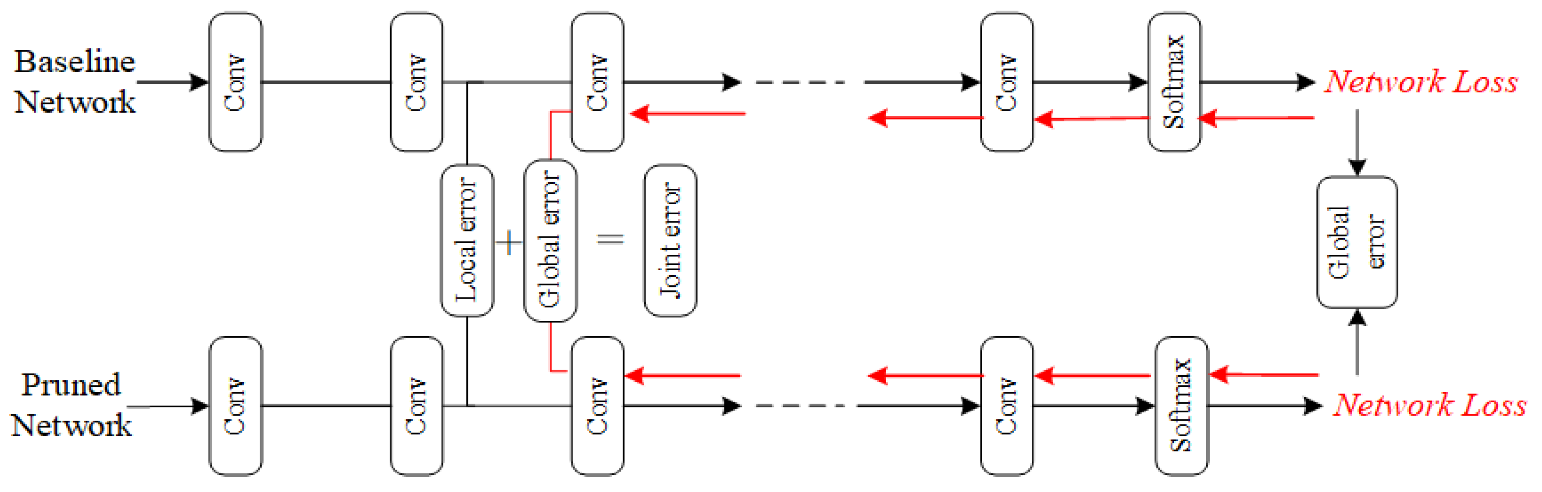
In this paper, we try to measure the importance of channels from both local and global aspects. The proposed JRE method can not only ensure the integrity of information in the forward propagation process but also ensure the discrimination ability of the model. That is, the functionality of the model itself does not decline. To preserve the discrimination ability of the neural network from a global perspective, we add the global reconstruction error to the neural network. Because other operations (such as normalization, ReLU activation function, maximum pooling, etc.) in convolution neural networks do not play a role in feature extraction, we assume that the feature information is transmitted directly between the convolution layers when calculating the local reconstruction error. The proposed channel pruning method based on joint reconstruction error is shown in
Figure 1.
As shown in
Figure 1, the baseline network and the pruned network are symmetrical to each other. The local error represents our proposed local reconstruction error, and the global error represents our proposed global reconstruction error. We will select channels based on joint errors calculated by local reconstruction errors and global reconstruction errors. The Network Loss (
NL) in
Figure 1 is the loss of the whole network, which will be used to calculate the global reconstruction errors in the back propagation process.
3.2. Local Reconstruction Error
Local reconstruction errors ensure that the integrity of information in the forward propagation process of the network. We try to find such a set of convolution kernels from the convolution layer to satisfy Formula (2),
where
represents the output feature map of the
ith layer of the benchmark model
b,
represents the output feature map of the
ith layer of the model after pruning, and j represents the remaining channels. The formula means that we are trying to select a set of kernels in the
ith layer of the baseline model so that the F-norm between
and
is the minimum, which ensures that nonessential channels are pruned. Because selecting a series of combinations that satisfy formulas from hundreds of kernels in a layer requires a lot of computing resources, we reduce the amount of calculation by equating Formula (2) with Formula (3),
where
represents the output feature map calculated from the pruned convolution kernels in the ith layer of the model and P represents the eliminated channel. The problem of finding preserved kernels in Formula (2) is transformed into a problem of finding pruned kernels, which reduces the scale of the problem. The local reconstruction error can be calculated by Formula (4).
The local reconstruction error represents the channel importance score based on a local calculation. Since other operations in the network (such as normalization, Sigmoid activation function, maximum pooling, etc.) do not perform feature extraction, when calculating the local channel importance score, we assume that the information is the direct transmission between convolution layers. That is, the importance of layers other than convolution is not considered.
3.3. Global Reconstruction Error
The global reconstruction error guarantees the discrimination ability of the model. That is, the functionality of the model itself does not decline. We sought to find such a set of convolution kernels to satisfy Formula (5),
where
represents the difference of the Network Loss (
) before and after channel
h is pruned.
represents the Network Loss (
) value when channel
h is 0. That is, the loss function value of channel
h is pruned. In addition,
represents the
value when channel
h is
. Curve fitting is introduced into Formula (5), as shown in Formula (6).
Complex neural networks usually have a large number of random parameters, so it is difficult to make neural networks before and after pruning reach the same state. Therefore, the first-order Taylor expansion formula is introduced, the function
is expanded at
, and all except the first-order terms are discarded to obtain the first-order Taylor expansion of
at
h = 0, as shown in Formula (7).
Bring Formula (7) into Formula (6) to obtain Formula (8),
where
represents the gradient of the loss function for
during back propagation. Our demand is transformed into finding such a channel
h, and the product of its value and its corresponding back-propagation gradient is close to 0. If the product of the value of the channel
h and its corresponding back-propagation gradient is close to 0, the channel
h has little effect on the discrimination ability of the neural network. The global reconstruction error can be calculated by Formula (9).
where
represents the channel importance score based on global calculation. When the score is smaller, it indicates that the kernel is less important and vice versa. The global reconstruction error
reflects the importance of a channel to the whole model.
3.4. Joint Loss Function
Due to the magnitude of the global reconstruction error and the local reconstruction error being different, we use the normalization method to calculate the joint loss function. The global reconstruction error is normalized by Formula (10).
The local reconstruction error is normalized by Formula (11), and the joint error can be obtained by Equation (12).
3.5. Channel Pruning Based on Joint Reconstruction Error
The proposed JRE method can be described by Algorithm 1. Start with the pre-trained model M and take stage i as an example. Feature maps propagate forward layer by layer in the network. Algorithm 1 first determines whether the layer is a convolution layer. If it is a convolution layer, is calculated by Formula (4). Then, is calculated by Formula (9) during back propagation, and finally, the joint error L is calculated by Formula (12). Prune the pre-trained model M according to the ascending sorting result of L.
In addition, because fine tuning is very important to compensate the accuracy loss of model M to suppress the cumulative error, we add fine tuning at the end of Algorithm 1.
At each stage, we calculate the importance (joint error
L) of each channel in model M and then sort the importance, so the pruning rate ratios of different layers can be potentially included in our method. We do not need to analyze the sensitivity of each layer to pruning nor do we need to manually define the pruning rate ratio of different layers. We only need to predefine a desired global pruning rate before the model pruning operation. When the global pruning rate is reached, the pruning operation will stop automatically.
| Algorithm 1: Channel pruning |
![Symmetry 14 01372 i001]() |


