A Modified Stein Variational Inference Algorithm with Bayesian and Gradient Descent Techniques

Abstract

This paper introduces a novel variational inference (VI) method with Bayesian and gradient descent techniques. To facilitate the approximation of the posterior distributions for the parameters of the models, the Stein method has been used in Bayesian variational inference algorithms in recent years. Unfortunately, previous methods fail to either explicitly describe the influence of its history in the tracing of particles ($Q\left(x\right)$ in this paper) in the approximation, which is important information in the search for particles. In our paper, $Q\left(x\right)$ is considered in design of the operator ${\mathcal{B}}_p$, but the chance of jumping out of the local optimum may be increased, especially in the case of complex distribution. To address the existing issues, a modified Stein variational inference algorithm is proposed, which can make the gradient descent of Kullback–Leibler (KL) divergence more random. In our method, a group of particles are used to approximate target distribution by minimizing the KL divergence, which changes according to the newly defined kernelized Stein discrepancy. Furthermore, the usefulness of the suggested technique is demonstrated by using four data sets. Bayesian logistic regression is considered for classification. Statistical studies such as parameter estimate classification accuracy, $F_1$, NRMSE, and others are used to validate the algorithm’s performance.

1. Introduction

In the area of inference issues, variational approaches [1] have lately gained popularity as a way to find a symmetric or asymmetric distribution that is close to the correct posterior from a simple class of distributions. The roots of variational inference (VI) can be traced back to the 1980s, describing mean-field methods, and play a key role in statistical mechanics. Variational approaches have a wide range of applications in Bayesian inference on asymmetric distribution [2], parameter-learning research [3,4,5,6,7], neural networks [8,9], and probabilistic graphical models [10]. To approximate the entire posterior, variational approaches try to reduce the Kullback–Leibler divergence [11] between the genuine posterior and a preset factorized distribution on the same variables. This method aims to find an approximation distribution $Q(\mathbf{x};\theta )$ over variables $\mathbf{x}$ to estimate the actual distribution $P\left(\mathbf{x}\right)$, and to describe the “degree of similarity” as the KL divergence $KL\left[Q\right(\mathbf{x};\theta )\parallel P(\mathbf{x}\left)\right]$ [12].

The VI method belongs to the optimization-based techniques category of approximate Bayesian inference. Methods are also available in this aspect of the research work, such as loopy belief propagation [13] and expectation propagation [14,15]. These optimization methods are typically faster, but they can suffer from a local optimum in posterior approximations. As we all know, the sampling method can effectively simplify the calculation program. The Markov chain Monte Carlo (MCMC) method [16,17,18] is generally unbiased in design, so it converges to the true posterior in the upper limit, but the process is slow. There has been significant development in both disciplines [19,20,21], focusing on closing the gap between these methodologies [22,23]. Indeed, recent success in scalable VI is based on combining optimization and sampling methods.

These years, the availability of enormous data sets has sparked interest in scalable methods. Different new VI methods have been proposed that differ significantly from earlier formulations. In reference [24], SVI is presented for models belonging to the conditionally conjugate exponential family. In reference [25], the BBVI framework is proposed, which focuses primarily on a single framework that is implemented in a black box form to allow scalability and ease of use. In reference [26], the latent variables are estimated as functions of inference networks, allowing DGPs to expand to larger data sets, accelerating the convergence rate. In references [27,28], the Gumbel-max trick and substituting the argmax operation with a softmax operator are used to approximate the categorical distribution.

Stein’s method is a particle approximation strategy [29,30] and a smart optimization method that can avoid the local posterior. It is a criterion for determining how well one approximate distribution matches another one. The Stein discrepancy method has been used in modern VI [31,32]. There are two representative methods: the Stein variational gradient descent (SVDG) [32] and operator VI [33]. Although both strategies have the same goal, they are optimized differently. However, these optimization-based approaches are often quicker, but they may be afflicted with a local optimum in posterior approximations. To deal with this issue, it is necessary to propose an modified Stein discrepancy method. The contribution of this paper can be summarized as follows:

(1)

The modified Stein variational gradient descent method (MSVGD) algorithm is proposed, in which an improved Stein method is used in a gradient increment calculation of KL divergence. A set of particles are used to approximate target distribution by minimizing the KL divergence;

(2)

The SVGD algorithm can keep the KL value reduced in the gradient descent theory. $K(\mathbf{x},·)$ is only in the unit ball of a reproducing kernel Hilbert space (RKHS). The SVGD algorithm will become slow in searching for the parameter distribution because of the limitation of local optimization. It is quite hard to jump out of the local optimum using the SVGD algorithm. In the referece [31], Stein’s operator is based on $K(\mathbf{x},·)$. Considering $Q\left(x\right)$ in the design of the ${\mathcal{B}}_p$ operator can increase the chance to jump out of the local optimum, especially in the case of complex distribution.

The rest of this paper is organized as follows. Section 2 describes model formulation and preliminaries. In Section 3, a modified Stein variational inference method is introduced for posteriori probability selection. In Section 4, experiments are carried out utilizing synthetic and publicly available data. The suggested method’s performance is analyzed and compared with that of various other popular methodologies.

2. Model Formulation and Preliminaries

2.1. Stein Method

The Stein approach can be described as follows for a target distribution P. Select a suitable Stein operator $\mathcal{B}:={\mathcal{B}}_P$ and a suitable Stein class of functions ${\mathcal{F}}_{\mathcal{B}}=\mathcal{F}\left({\mathcal{B}}_P\right)$ so that Z has distribution P, denoted $Z\sim P$. X has distribution Q, denoted $X\sim Q$. For all functions $f\in {\mathcal{F}}_{\mathcal{B}}$, we obtain the expectation

$$\mathbb{E}\left[\mathcal{B}f\right(Z\left)\right]=0.$$

Stein presents a metric for determining how close the rules of distribution P and Q are in reference [29]. For a measure class of functions in Hilbert space($\mathcal{H}$), ∀$r\in {\mathcal{F}}_{\mathcal{H}}$, a solution $f\in {\mathcal{F}}_{\mathcal{B}}$ can be found

$$r\left(X\right)-\mathbb{E}\left[r\right(Z\left)\right]=\mathcal{B}f\left(X\right).$$

(1)

Taking expectations of (1), we have

$$\mathbb{E}\left[r\right(X\left)\right]-\mathbb{E}\left[r\right(Z\left)\right]=\mathbb{E}\left[\mathcal{B}f\right(X\left)\right].$$

Probability distances $r\left(X\right)$ and $r\left(Z\right)$ can be written as

$$S(X,Z)=\underset{r\in {\mathcal{F}}_{\mathcal{H}}}{sup}|\mathbb{E}\left[r\left(X\right)\right]-\mathbb{E}\left[r\left(Z\right)\right]|$$

see reference [29] for an overview. Hence, we get

$$S(X,Z)\le \underset{f\in {\mathcal{F}}_{\mathcal{B}}}{sup}\left|\mathbb{E}\left[\mathcal{B}f\left(X\right)\right]\right|,$$

where f is the solutions of (1) for functions in ${\mathcal{F}}_{\mathcal{B}}$. The primary idea behind Stein’s technique is to select an appropriate $S(X,Z)$.

2.2. Variational Inference

In variational inference, the Kullback–Leibler (KL) divergence is utilized for two distributions, $P\left(\mathbf{x}\right)$ and $Q\left(\mathbf{x}\right).$ VI is the process of minimizing the difference between two distributions, also known as relative entropy or information gain.

$$\begin{array}{cc}\hfill D_{KL}(Q\left(\mathbf{x}\right)\parallel P\left(\mathbf{x}\right))& =-\int Q\left(\mathbf{x}\right)log\frac{P\left(\mathbf{x}\right)}{Q\left(\mathbf{x}\right)}dz\hfill \\ \hfill & =-{\mathbb{E}}_{Q\left(\mathbf{x}\right)}\left[log\frac{P\left(\mathbf{x}\right)}{Q\left(\mathbf{x}\right)}\right].\hfill \end{array}$$

By reducing the KL divergence, the target distribution $P\left(\mathbf{x}\right)$ is approximated by VI with proposal distribution $Q\left(x\right)$. A more straightforward distribution $Q^{*}\left(\mathbf{x}\right)$ comes from a predetermined set $\mathbf{Q}$ $=\left\{Q\right(\mathbf{x}\left)\right\}$ of proposal distributions. $Q^{*}\left(\mathbf{x}\right)$ can be written as

$$Q^{*}\left(\mathbf{x}\right)=\underset{q\in \mathcal{Q}}{\arg \min }\left\{D_{KL}(Q\left(\mathbf{x}\right)\parallel P\left(\mathbf{x}\right))\equiv {\mathbb{E}}_Q[logQ\left(\mathbf{x}\right)]-{\mathbb{E}}_Q[logP\left(\mathbf{x}\right)]\right\}.$$

(2)

According to the above formula, our main work is to solve the formula ${\mathbb{E}}_Q[logQ\left(\mathbf{x}\right)]$. However, from the formula, we can not perform this directly. The selection of set $\mathbf{Q}$ is crucial, as it determines the types of variational methods that can be used. The optimal $\mathbf{Q}$ should strike a compromise between $P\left(\mathbf{x}\right)$ accuracy, $Q\left(\mathbf{x}\right)$ tractability, and KL minimization solvability.

We need to identify a set $\mathbf{Q}$ of distributions derived from a tractable reference distribution using smooth transformations. Assume $\mathbf{Q}$ is a set of random variable distributions of the form $z=F\left(\mathbf{x}\right)$, and F is a measurable smooth linear function. $\mathbf{x}$ is selected from a tractable reference distribution $Q\left(\mathbf{x}\right)$. z can be written as

$$z=Q\left(F^{-1}\left(z\right)\right)·\left|{\nabla }_z{F}^{-1}\left(z\right)\right|,$$

where ${\nabla }_z{F}^{-1}$ is the Jacobian matrix of $F^{-1}$.

3. Modified Stein Variational Inference Using KL Minimizing

3.1. Stein Operators Selection

There are various ways of constructing a Stein operator [31,32]. Our model is based on Stein’s identity and the kernelized Stein discrepancy. Assume that $P\left(\mathbf{x}\right)$ and $Q\left(\mathbf{x}\right)$ are all smooth density, where $Q\left(\mathbf{x}\right)={\left[Q_1\left(\mathbf{x}\right),\cdots ,Q_d\left(\mathbf{x}\right)\right]}^{\top }$, $\mathbf{x}\subseteq {\mathbb{R}}^d$. According to characteristics of the Stein method, we get suitably regular $\varphi \left(\mathbf{x}\right)={\left[{\varphi }_1\left(\mathbf{x}\right),\cdots ,{\varphi }_d\left(\mathbf{x}\right)\right]}^{\top },$ and suitably

$${\mathbb{E}}_{\mathbf{x}\sim P}\left[{\mathcal{B}}_P\varphi \left(\mathbf{x}\right)Q\left(\mathbf{x}\right)\right]=0,$$

(3)

where

$${\mathcal{B}}_P\varphi \left(\mathbf{x}\right)Q\left(\mathbf{x}\right)=Q{\left(\mathbf{x}\right)}^{\top }\varphi {\left(\mathbf{x}\right)}^{\top }{\nabla }_{\mathbf{x}}logP\left(\mathbf{x}\right)+{\nabla }_{\mathbf{x}}\varphi \left(\mathbf{x}\right)Q\left(\mathbf{x}\right)+{\nabla }_{\mathbf{x}}Q\left(\mathbf{x}\right)\varphi \left(\mathbf{x}\right).$$

${\mathcal{B}}_p$ has an effect on the function $\varphi \left(\mathbf{x}\right)Q\left(\mathbf{x}\right)$ and produces the zero mean function ${\mathcal{B}}_P\varphi \left(\mathbf{x}\right)Q\left(\mathbf{x}\right)$. $\varphi \left(\mathbf{x}\right)$ is in the Stein class of distribution $P.$ $\forall \mathbf{x}\subseteq \partial A$, set $A\subset {\mathbb{R}}^d$ is compact, $P\left(\mathbf{x}\right)Q\left(\mathbf{x}\right)\varphi \left(\mathbf{x}\right)\approx 0$. It is obviously that the expectation of ${\mathcal{B}}_P\varphi \left(\mathbf{x}\right)Q\left(\mathbf{x}\right)$ is not equivalent to 0 any longer. The magnitude of ${\mathbb{E}}_{\mathbf{x}\sim Q}\left[{\mathcal{B}}_P\varphi \left(\mathbf{x}\right)Q\left(\mathbf{x}\right)\right]$ is related with the probability distances between P and Q. The probability distances of $Q,P$ are referred to as follows:

$$S(Q,P)=\underset{\varphi \in {\mathcal{F}}_{\mathcal{B}}}{max}\left\{{\left[{\mathbb{E}}_{\mathbf{x}\sim Q}trace\left({\mathcal{B}}_P\varphi \left(\mathbf{x}\right)Q\left(\mathbf{x}\right)\right)\right]}^2\right\},$$

where ${\mathcal{F}}_{\mathcal{B}}$ is a set of functions with bounded Lipschitz norms. However, optimization leads to the unsolvable challenge of $S(Q,P)$ in calculation. We need to come up with a solution that is both reasonable and feasible.

In (4), the kernelized Stein discrepancy (KSD) and variational inference method is used that select $Q\left(\mathbf{x}\right)$ and $\varphi \left(\mathbf{x}\right)$ in the unit ball of a reproducing kernel Hilbert space (RKHS). In RKHS, $\mathbb{S}(Q,P)$ is written as

$$S(Q,P)=\underset{\varphi \in {\mathcal{H}}^d}{max}\left\{{\left[{\mathbb{E}}_{\mathbf{x}\sim Q}\left(trace\left({\mathcal{B}}_P\varphi \left(\mathbf{x}\right)Q\left(\mathbf{x}\right)\right)\right)\right]}^2,\mathrm{s}.\mathrm{t}.{\parallel \varphi \left(\mathbf{x}\right)Q\left(\mathbf{x}\right)\parallel }_{{\mathcal{H}}^d}\le 1\right\}.$$

(4)

Let $\psi \left(\mathbf{x}\right)=\varphi \left(\mathbf{x}\right)Q\left(\mathbf{x}\right)$, and the optimal solution of (4) can be represented by $\psi \left(\mathbf{x}\right)={\psi }^{*}\left(\mathbf{x}\right)/{∥{\psi }^{*}\left(\mathbf{x}\right)∥}_{{\mathcal{H}}^d}$, ${\psi }_{Q,P}^{*}(·)={\mathbb{E}}_{\mathbf{x}\sim Q}\left[{\mathcal{B}}_{P}K(\mathbf{x},·)Q\left(\mathbf{x}\right)\right].$ $K\left(\mathbf{x},{\mathbf{x}}^{\prime }\right)$ is the function of ${\mathcal{F}}_{\mathcal{B}}$ in RKHS. Obviously, $S(Q,P)$ can written as

$$S(Q,P)={∥{\psi }_{Q,P}^{*}∥}_{{\mathcal{H}}^d}^2.$$

(5)

According to the above information, when P equals to Q, $S(Q,P)=0$, ${\psi }_{Q,P}^{*}\left(\mathbf{x}\right)\equiv 0$. We aim to find a distribution that is close to $P.$ In other words, $S(Q,P)$ approximates to zero.

3.2. Stein Transform for Differential Computing of KL

Add a small disturbance to the linear transform in (2) to reduce the KL divergence: $F\left(\mathbf{x}\right)=\omega \mathbf{x}+\epsilon \psi \left(\mathbf{x}\right),$ where $\omega$ is a constant, $\epsilon$ is the magnitude of the disturbance, and $\psi \left(\mathbf{x}\right)$ is a continuously differentiable function that describes the direction of the disturbance. The Jacobian matrix of $F\left(\mathbf{x}\right)$ is non-singular when $\epsilon$ is small enough, so the inverse function theorem guarantees that F is a linear function. The following conclusion, as the basis for our method, establishes a useful link between the ${\mathcal{B}}_P$ and the differential of KL.

Theorem 1.

Define $F\left(\mathbf{x}\right)=\omega \mathbf{x}+\epsilon \psi \left(\mathbf{x}\right)$. $Q_{\left[F\right]}\left(z\right)$ is the probability density function (pdf) of $z=F\left(\mathbf{x}\right).$ The pdf of $\mathbf{x}$ is $Q\left(\mathbf{x}\right).$ We will prove that

$${\nabla }_{\epsilon }\mathrm{KL}{\left(Q_{\left[F\right]}\parallel P\right)}_{\epsilon =0}=-{\mathbb{E}}_{\mathbf{x}\sim Q}\left[trace\left({\omega }^{-1}{\mathcal{B}}_P\psi \left(\mathbf{x}\right)\right)\right],$$

(6)

where ${\mathcal{B}}_P\psi \left(\mathbf{x}\right)=\varphi \left(\mathbf{x}\right)Q\left(\mathbf{x}\right){\nabla }_{\mathbf{x}}logP{\left(\mathbf{x}\right)}^{\top }+{\nabla }_{\mathbf{x}}\varphi \left(\mathbf{x}\right)Q\left(\mathbf{x}\right)+{\nabla }_{\mathbf{x}}Q\left(\mathbf{x}\right)\varphi \left(\mathbf{x}\right)$ is a differential operator (called Stein operator). From (4) and (5), ${\mathcal{B}}_P\psi \left(\mathbf{x}\right)$ can be used to show how fast KL divergence is deteriorating in RKHS.

Proof. 

From the definition, Q and P are all smooth pdf, and $z=F\left(\mathbf{x}\right)$, a linear transform with parameter $\epsilon$, which is differentiable with respect to both $\mathbf{x}$ and $\epsilon$. $Q_{\left[F\right]}$ is the pdf of z; $Q\left(\mathbf{x}\right)$ is the pdf of $\mathbf{x}$; and $Q_{\left[F^{-1}\right]}\left(\mathbf{x}\right)$ is the pdf of $\mathbf{x}=F^{-1}\left(z\right)$ and can also be represented as

$$Q_{\left[F^{-1}\right]}\left(\mathbf{x}\right)=Q\left(F\left(\mathbf{x}\right)\right)·\left|det\left({\nabla }_{\mathbf{x}}F\left(\mathbf{x}\right)\right)\right|.$$

From the KL definition, it is very obvious that

$$\mathrm{KL}\left(Q_{\left[F\right]}\parallel P\right)=\mathrm{KL}\left(Q\parallel P_{\left[F^{-1}\right]}\right),$$

$${\nabla }_{\epsilon }\mathrm{KL}\left(Q_{\left[F\right]}\parallel P\right)=-{\mathbb{E}}_{\mathbf{x}\sim Q}\left[{\nabla }_{\epsilon }log{P}_{\left[F^{-1}\right]}\left(\mathbf{x}\right)\right].$$

We can easily obtain

$${\nabla }_{\epsilon }log{P}_{\left[F^{-1}\right]}\left(\mathbf{x}\right)=\frac{1}{P\left(F\right(\mathbf{x}\left)\right)}{\nabla }_{F\left(\mathbf{x}\right)}P\left(F\left(\mathbf{x}\right)\right){\nabla }_{\epsilon }F\left(\mathbf{x}\right)+trace\left({\left({\nabla }_{\mathbf{x}}F\left(\mathbf{x}\right)\right)}^{-1}·{\nabla }_{\epsilon }{\nabla }_{\mathbf{x}}F\left(\mathbf{x}\right)\right).$$

Let $s_P\left(F\left(\mathbf{x}\right)\right)={\nabla }_{F\left(\mathbf{x}\right)}logP\left(F\left(\mathbf{x}\right)\right),$ and we get

$${\nabla }_{\epsilon }log{P}_{\left[F^{-1}\right]}\left(\mathbf{x}\right)=s_P{\left(F\left(\mathbf{x}\right)\right)}^{\top }{\nabla }_{\epsilon }F\left(\mathbf{x}\right)+trace\left({\left({\nabla }_{\mathbf{x}}F\left(\mathbf{x}\right)\right)}^{-1}·{\nabla }_{\epsilon }{\nabla }_{\mathbf{x}}F\left(\mathbf{x}\right)\right).$$

When $F\left(\mathbf{x}\right)=\omega \mathbf{x}+\epsilon \varphi \left(\mathbf{x}\right)Q\left(\mathbf{x}\right)$ and $\epsilon =0$, the result is obtained is as follows:

$$F\left(\mathbf{x}\right)=\omega \mathbf{x},{\nabla }_{ϵ}F\left(\mathbf{x}\right)=\psi \left(\mathbf{x}\right),{\nabla }_{\mathbf{x}}F\left(\mathbf{x}\right)=\omega I,{\nabla }_{\epsilon }{\nabla }_{\mathbf{x}}F\left(\mathbf{x}\right)={\nabla }_{\mathbf{x}}\psi \left(\mathbf{x}\right).$$

Based on Theorem 1, the KSD $-\mathbb{S}(Q,P)$ is equal to

$${\nabla }_{\epsilon }\mathrm{KL}{\left(Q_{\left[F\right]}\parallel P\right)}_{\epsilon =0}\prime$$

and ${\psi }_{Q,P}^{*}(·)$ can also be written as

$${\psi }_{Q,P}^{*}(·)={\mathbb{E}}_{\mathbf{x}\sim Q}\left[K(\mathbf{x},·)Q\left(\mathbf{x}\right){\nabla }_{\mathbf{x}}logP\left(\mathbf{x}\right)+{\nabla }_{\mathbf{x}}\left(K(\mathbf{x},·)Q\left(\mathbf{x}\right)\right)\right].$$

(7)

With the conclusion drawn from above, ${\nabla }_{\epsilon }\mathrm{KL}{\left(Q_{\left[F\right]}\parallel P\right)}_{\epsilon =0}$ is the decreasing direction of KL divergence. $F\left(\mathbf{x}\right)$ is a linear transform, so $F\left(\mathbf{x}\right)=\omega \mathbf{x}+\epsilon ·{\psi }_{Q,P}^{*}\left(\mathbf{x}\right)$ is selected as a method which can decrease the KL divergence, where $\epsilon$ is a small constant.

According to the gradient descent theory, the decreasing direction of ${\nabla }_{\epsilon }\mathrm{KL}{\left(Q_{\left[F\right]}\parallel P\right)}_{\epsilon =0}$ is fastest, and the local or global optimal Q must be found. Q is initialized as $Q_0$. Repeating the (8) steps, a distribution set ${\left\{Q_{\ell }\right\}}_{\ell =1}^n$ is generated

$$Q_{\ell +1}=Q_{\ell \left[F_i\right],},\mathrm{where}{F}_{\ell }^{*}\left(\mathbf{x}\right)=\omega \mathbf{x}+{\epsilon }_{\ell }·{\psi }_{Q,P}^{*}\left(\mathbf{x}\right).$$

(8)

From (8), we see that $Q_{\ell }$ can converge to distribution P with arbitrarily small ${\epsilon }_{\ell }$ and a given $\omega$. When $\ell \to \infty$, $Q_{\ell }=P$ and ${\psi }_{P,Q_{\infty }}^{*}\left(\mathbf{x}\right)\equiv 0$.    □

3.3. Modified Stein Variational Gradient Descent Method with Particle Swarm Optimization

To compute ${\nabla }_{\epsilon }\mathrm{KL}{\left(Q_{\left[F\right]}\parallel P\right)}_{e=0}$, we would need to calculate ${\psi }_{Q,P}^{*}\left(\mathbf{x}\right)$ in (7). Particle swarm optimization is used to approximate the target distribution $P\left(\mathbf{x}\right)$ with the stochastic gradient descent method.

To begin, we will need to create a collection of particles ${\left\{{\mathbf{x}}_i^0\right\}}_{i=1}^n$ from the initial distribution Q. ${\psi }_{Q,P}^{*}\left(\mathbf{x}\right)$ and Q are approximated by the empirical mean of particles at the last iteration of Formula (8). The value of parameter $\omega$ can also affect Algorithm 1’s effectiveness, but the emphasis of the algorithm lies in the application of the Stein variational inference in system identification, so $\omega =1$ is selected for the moment, and other values of $\omega$ are not discussed for the time being. As n increases, ${\left\{{\mathbf{x}}_i^0\right\}}_{i=1}^n$ becomes a better approximation for $Q_i$.

For any fixed $i_0,$ the distribution of each particle ${\mathbf{x}}_{i_0}^{\ell },$ tends to $Q_i,$ and is unaffected by any other finite group of particles.

In Algorithm 1, the first part in ${\psi }_{Q,P}^{*}(·)$ pushes the particles towards the direction where the probability $P\left(\mathbf{x}\right)$ increases rapidly with the kernel function $K\left(\mathbf{x},{\mathbf{x}}^{\prime }\right)$ and distribution $Q_i$. The second part prevents any of the particles from collapsing into local maximization. The radial basis function (RBF) kernel $K\left(\mathbf{x},{\mathbf{x}}^{\prime }\right)=exp\left(-\frac{1}{\rho }{∥\mathbf{x}-{\mathbf{x}}^{\prime }∥}^2\right)$ is considered in our paper. As ${\sum }_j{\nabla }_{{\mathbf{x}}_j}Q\left({\mathbf{x}}_j\right)K\left({\mathbf{x}}_j,\mathbf{x}\right)$ reaches zero, the second term

Algorithm 1 Modified Stein Variational Gradient Descent Method (MSVGD)

Input:    A group of random particles ${\left\{{\mathbf{x}}_i^0\right\}}_{i=1}^n$ and target pdf $P\left(\mathbf{x}\right)$    Set the initial state of particles ${\mathbf{x}}_i^t$, constant parameter $\omega$, step size ${\epsilon }_t$. 1: for iteration t do 2:    ${\mathbf{x}}_i^{t+1}\leftarrow \omega {\mathbf{x}}_i^t+{\epsilon }_t{\widehat{\psi }}^{*}\left({\mathbf{x}}_i^t\right)$ where $${\widehat{\psi }}^{*}\left(\mathbf{x}\right)=\frac{1}{n}\sum _{j=1}^n\left[K\left({\mathbf{x}}_j^t,\mathbf{x}\right)Q\left({\mathbf{x}}_j^t\right){\nabla }_{{\mathbf{x}}_j^t}logP\left({\mathbf{x}}_j^t\right)+{\nabla }_{{\mathbf{x}}_j^t}K\left({\mathbf{x}}_j^t,\mathbf{x}\right)Q\left({\mathbf{x}}_j^t\right)\right]$$ (9) 3:    break 4: end for Output:    The particles ${\left\{{\mathbf{x}}_i\right\}}_{i=1}^n$ that tries to match the goal distribution $P\left(\mathbf{x}\right)$.

$$\sum _j\frac{2}{\tau }\left(\mathbf{x}-{\mathbf{x}}_j\right)k\left({\mathbf{x}}_j,\mathbf{x}\right)Q\left({\mathbf{x}}_j\right)+\sum _j{\nabla }_{{\mathbf{x}}_j}Q\left({\mathbf{x}}_j\right)k\left({\mathbf{x}}_j,\mathbf{x}\right)$$

(10)

decreases. Clearly, the second term pushes $\mathbf{x}$ away from neighboring points ${\mathbf{x}}_j$ with high $K\left({\mathbf{x}}_j,\mathbf{x}\right)$. When the cumbersome term is weakened in the bandwidth $\rho \to 0$, the local optimum will be swiftly reached by all of the particles.

Our method is different to that of reference [32] in that the $Q\left(\mathbf{x}\right)$ is considered in the Stein operator design, which reflects the influence of distribution change on the results. This attribute sets our method apart from traditional Monte Carlo methods. Obtaining a diverse set of points for distributional approximation is a random process.

3.4. MSVGD Algorithm and Its Computational Difficulty

Algorithm 1 is where the MSVGD algorithm’s core procedure takes place. The inertia weight $\omega$ in this technique can fluctuate depending on the previous particle position. However, the value of $\omega$ is limited to 1, which is neither too big or small. For all the points ${\left\{{\mathbf{x}}_i\right\}}_{i=1}^n$, the main work in this algorithm is to determine the gradient $Q\left(\mathbf{x}\right){\nabla }_{\mathbf{x}}logP\left(\mathbf{x}\right)$ for all of the points. $P\left(\mathbf{x}\right)\propto P_0\left(\mathbf{x}\right){\prod }_{k=1}^{N}P\left(D_k\mid \mathbf{x}\right)$ is accompanied by a broad N. Approximating $Q\left(\mathbf{x}\right){\nabla }_{\mathbf{x}}logP\left(\mathbf{x}\right)$ with a small piece of sampled data $\mathsf{\Lambda }\subset \{1,\dots ,N\}$ is a convenient way to deal with this issue. The formula is written as

$$Q\left(\mathbf{x}\right){\nabla }_{\mathbf{x}}logP\left(\mathbf{x}\right)\approx Q_0\left(\mathbf{x}\right){\nabla }_{\mathbf{x}}log{P}_0\left(\mathbf{x}\right)+\frac{N}{\left|\mathsf{\Lambda }\right|}Q(\left(D_k\mid \mathbf{x}\right)\sum _{k\in \mathsf{\Lambda }}{\nabla }_{\mathbf{x}}logP\left(D_k\mid \mathbf{x}\right).$$

The computational complexity of the original VI algorithm is easy to obtain, represented by $O(n·n)$.

In the MSVGD algorithm, the entire computational difficulty caused by the computation of the $K(\mathbf{x},·)Q\left(\mathbf{x}\right)$, which is denoted as $O(n·n·K(\mathbf{x},·\left)Q\right(\mathbf{x}\left)\right)$. $K(\mathbf{x},·)$ is the RBF kernel, and $Q\left(\mathbf{x}\right)$ is the approximation function of $P\left(\mathbf{x}\right)$. Assume $\tau =K(\mathbf{x},·)Q\left(\mathbf{x}\right)$, which is less than a constant ${\tau }_0$. $n\ast n$ is the same order of magnitude with ${\tau }_0\ast n\ast n$, so the total computational difficulty and runtime of MSVGD have no obvious difference with the original VI algorithm.

4. Numerical Examples

All empirical experiments using the MSVGD algorithm and other algorithms are conducted on the same platform in this study. Furthermore, we use the same software (Python 3.0 ) in the program running. The MSVGD algorithm can be used in other classification models (e.g., the neural network model, support vector machine, etc.). The framework of these methods is very similar to that of our example. In this study, we exclusively use the MSVGD algorithm to perform classification experiments with logistic regression. Following that, we will go into the specifics of the experiments. We create the data sets and methods that will be used in the comparison.

4.1. Experimental Setups

We use four data sets from UCI’s repository for logistic regression, including the Iris, Covertype, Pima, and heart disease data sets [34]. R.A. Fisher’s landmark paper employed the Iris data set. Multiple measures are used in taxonomic difficulties. Tree observations from four locations of Colorado’s Roosevelt National Forest are contained in the covertype data set. All of the data is derived from forest cartographic variables. The Pima data set contains medical records for Pima Indians, and whether each patient will develop diabetes in the next five years. Although the heart disease database has 76 features, a subset of 14 of them is used in all published trials. In particular, the Iris database is the only source of data with many classifications. In Section 4.1, we perform some tests on the MSVGD algorithm. Variational inference with the bound and Laplace’s approach [35] are two further methods for posterior approximation that we compare. We perform experiments for different corpus sizes.

The following MSVGD settings are used: (1) 6000 runs; (2) 50 particles in the population. (3) The MSVGD parameter w is increased from 0.7 to 1.3, with a 0.1 step length. In the two experiments, the $\mathrm{RBF}$ kernel $K\left(\mathbf{x},{\mathbf{x}}^{\prime }\right)=exp\left(-\frac{1}{\rho }{∥\mathbf{x}-{\mathbf{x}}^{\prime }∥}_2^2\right)$ is used with parameter $\rho$. The contribution point ${\mathbf{x}}^{\prime }$ to $\mathbf{x}$, which changes adaptively over iterations, is balanced by the value of $\rho$. Unless otherwise stated, for step size, we use AdaGrad, and for particle initialization, we use the prior distribution.

The selection behavior and prediction performance of each algorithm were our main concerns. For the former, we used the $F_1$ score (described below) to attain our goal.

$$F_1=\frac{2\times \mathrm{Precision}\times \mathrm{Recall}}{\mathrm{Precision}+\mathrm{Recall}},\mathrm{Precision}=\frac{\mathrm{TP}}{\mathrm{TP}+\mathrm{FP}},\mathrm{Recall}=\frac{\mathrm{TP}}{\mathrm{TP}+\mathrm{FN}}$$

The number of true positives, false positives, and false negatives is represented as TP, FP, and FN, respectively. The classification accuracy (Acc) is used to evaluate one method’s prediction ability. In general, $F_1$ and Acc have a range of 0 to 1, with larger values being desired. The normalized root mean square error (NRMSE) of logistic parameters is also taken into account.

$$NRMSE=\sqrt{\frac{1}{T{\sigma }^2}\underset{t=1}{\sum ^T}{({\theta }_t-\overline{\theta })}^2},$$

where T is the total number of tests, $\overline{\theta }$ is the mean parameter value, ${\theta }_t$ is the result of every experiment, and ${\sigma }^2$ denotes the variance of the results. In the following trials, we used a training data to learn the parameters in each model and presented the $F_1$ and NRMSE results for selection evaluation.

A test set of size 10,000 is independently produced with the goal of testing the inferred model’s prediction accuracy. In the case of each test instance $\mathbf{x}$, $p(y=1\mid \mathbf{x})$ is estimated in the logistic model. Setting threshold = $0.5$, we obtain $p(y=1\mid \mathbf{x})\ge 0.5$. On the test set, we then estimated the average accuracy to evaluate the prediction behavior of a method.

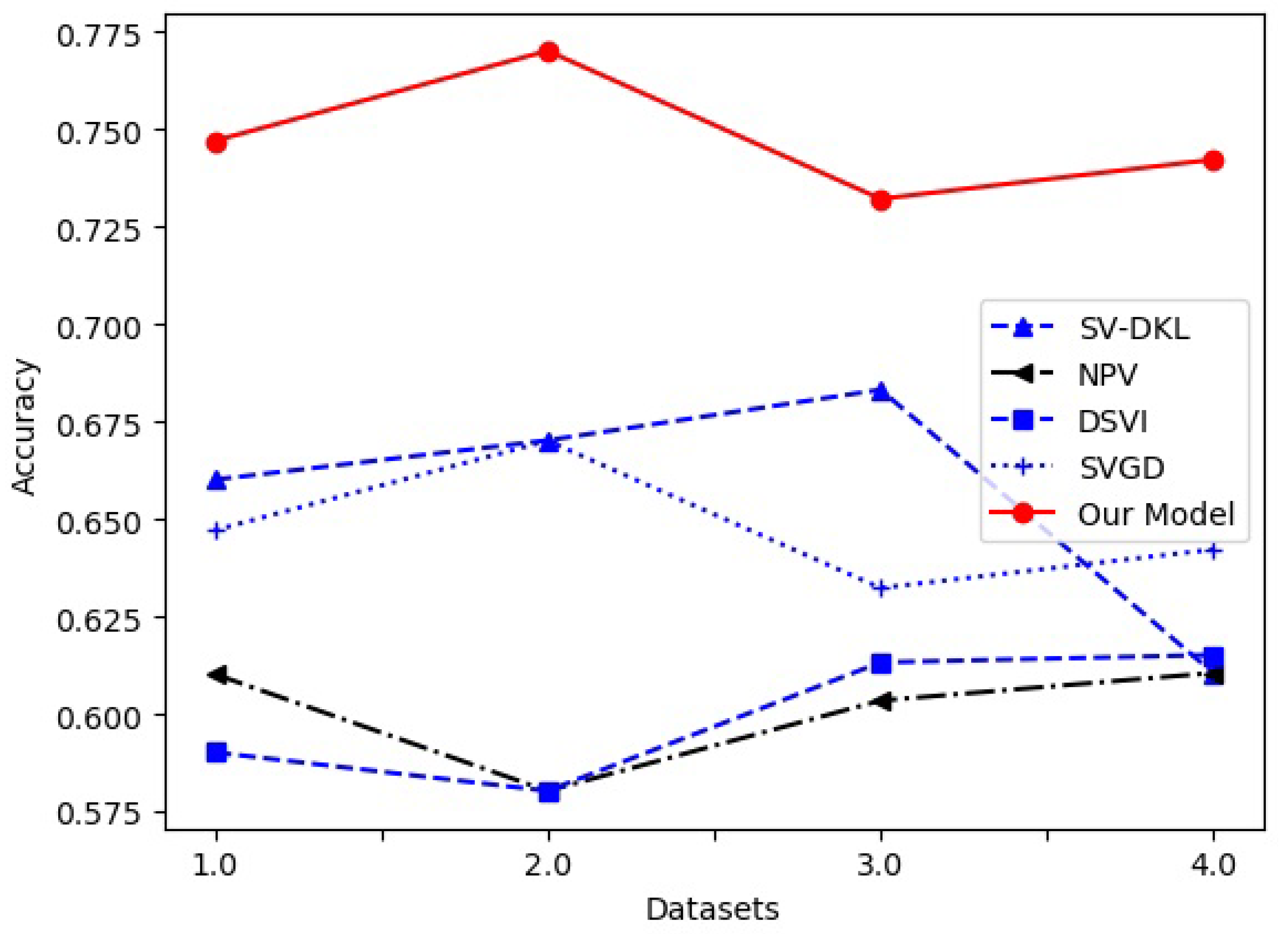
4.2. Comparison with Different VI Models in Five Data Sets

Bayesian logistic regression is considered for classification (binary and multi-) using the setting so that regression weights w have Gaussian prior $p_0(\eta \mid \alpha )=\mathcal{N}\left(\eta ,{\alpha }^{-1}\right)$ and $p_0\left(\alpha \right)=$ Gamma $(\alpha ,1,0.01)$ in the posterior $p(x\mid D)$, $x=[\eta ,log\alpha ]$. The accuracy of our model’s categorization on each data set is shown in

Table 1. Accuracy comparison of different VI methods.

Model Data		Iris	Pima	Covertype	Heart Disease	p-Value
SV-DKL [3]	Acc	0.6601	0.6702	0.6832	0.6104	0.010
	$F_1$	0.2662	0.2134	0.2361	0.2415
	$NRMSE$	0.6234	0.5915	0.6183	0.6453
	Average runtime (s)	29	28	72	34
NPV [5]	Acc	0.6102	0.5802	0.6034	0.6105	0.000
	$F_1$	0.3562	0.2536	0.2824	0.2713
	$NRMSE$	0.5235	0.5115	0.6355	0.5425
	Average runtime (s)	30	32	70	30
DSVI [6]	Acc	0.5901	0.5802	0.6132	0.6151	0.000
	$F_1$	0.2634	0.2456	0.2631	0.2514
	$NRMSE$	0.7235	0.6415	0.6883	0.7456
	Average runtime (s)	26	32	67	30
SVGD [31]	Acc	0.6471	0.6701	0.6323	0.6422	0.001
	$F_1$	0.4150	0.4456	0.4632	0.3815
	$NRMSE$	0.7136	0.7416	0.6114	0.7324
	Average runtime (s)	25	30	55	27
our model	Acc	0.7471	0.7702	0.7322	0.7423	0.000
	$F_1$	0.5151	0.5452	0.5634	0.5814
	$NRMSE$	0.6132	0.6414	0.6117	0.7345
	Average runtime (s)	15	16	34	18

. Since all methods yield an approximation of the posterior distribution on the vector x, this comparison is meaningful and provides a measure of parameter estimation.

For each data set, 80% of the data is chosen at random for training, and the rest is used for testing. The procedure is repeated 10 times, and the average accuracy is provided in Table 1. The results reveal that, compared with the latest method, our proposed method improves the performance by an average of 5%, which not only proves the effectiveness and efficiency of the proposed model, but also successfully finds the correlation and information adaptability.

Taking the Covertype data set as an example, we show performance details of the MSVGD algorithm in Figure 1, which is the results of the Bayesian logistic regression at different iterations. In Figure 2, the average classification accuracy of our model is best on Iris, Covertype, Pima, and heart disease for Bayesian logistic regression. In Table 1, we find that our method outperforms the other similar methods: SV-DKL [3], NPV [5], DSVI [6], and SVGD [31]. Although $NRMSE$ values in the two-test data (Covertype and heart disease) are not much different from our method, the value of $F_1$ and Acc in the MSVGD method is bigger than the others. The independent sample T-test method is used to examine the significance of data accuracy differences in Table 1. From Table 1, the p-values are all less than 0.05. In the four data sets, the average runtime of the MSVGD algorithm is 15 s, 16 s, 34 s, and 18 s, which is the shortest in all models. Based on these advantages, we can say that our method is better than the others.

4.3. Comparison with Different Non-VI Classification Models

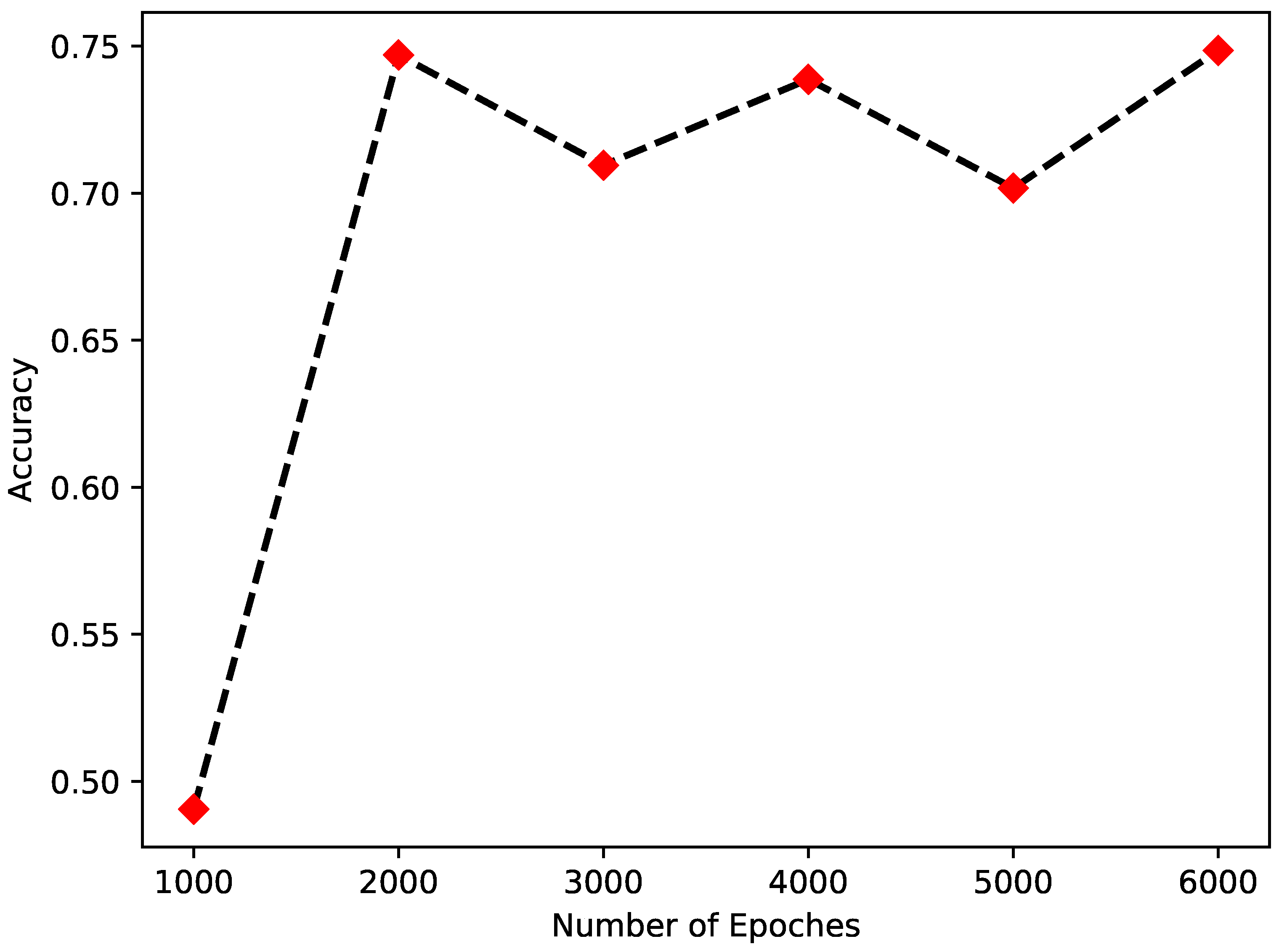
For classification tasks, the Stein method is applied to Bayesian inference. In the comparative analysis, we explore two prediction approaches in order to better investigate the benefits of the MSVGD algorithm in Bayesian logistic regression. The methods include the support vector machine (SVM) [36] and back propagation (BP) network [37]. From

Table 2. Accuracy comparison of different non-VI methods.

Model Data	Iris	Pima	Covertype	Heart Disease
SVM [3]	0.7212	0.7545	0.7221	0.7332
BP [5]	0.7061	0.7134	0.7124	0.7026
our model	0.7471	0.7702	0.7322	0.7423

, the Bayesian logistic regression outperforms the other approaches in terms of prediction accuracy. We concluded that the proposed strategy produces the best prediction performance after a brief visual evaluation. The results of the Bayesian logistic regression are superior to those of BP. The results of BP are inferior to SVM.

4.4. Analysis of Parameters $\omega$ and Function Q(x) in MSVGD Algorithm

Because of the adaptive nature of MSVGD, it outperforms other algorithms. In the MSVGD of the four data sets, the process of inertia weight swings around one, as seen in

Table 3. Accuracy comparison of different $\omega$ values.

$\mathit{\omega }$	Accuracy
	Iris	Pima	Covertype	Heart Disease
0.7	0.5514	0.5644	0.5431	0.5322
0.8	0.5764	0.5631	0.5624	0.5521
0.9	0.6562	0.6531	0.6721	0.6620
1.0	0.7061	0.7134	0.7124	0.7026
1.1	0.6762	0.6920	0.6811	0.6825
1.2	0.5861	0.5833	0.5922	0.5924
1.3	0.5471	0.5732	0.5621	0.5470

. We set the value of $\omega$ as an arithmetic sequence with a step size of 0.1, from 0.1 to 2. We can observe that approaching 1 has a similar or better performance than the rest. Table 3 is part of our result, where $\omega$ is between 0.7 and 1.3. $\omega$ mainly affects the particle positions at random, which control the convergence rate.

In the MSVGD, $Q\left(\mathbf{x}\right)$ is the past particle information. It is a function that influences the convergence rate, which can accelerate or slow the convergence of particles to the high-probability zones of $p\left(\mathbf{x}\right)$. In formula ${\widehat{\varphi }}^{*}\left(\mathbf{x}\right)$, the two terms are not only weighted by the kernel function, but also by $Q\left(\mathbf{x}\right)$. From the table, a smaller $Q\left(\mathbf{x}\right)$ means that the particles have more chances to change, but less information about previous particle positions is employed. Particle positions are less likely to change as $Q\left(\mathbf{x}\right)$ increases, and more previous particle position information is referenced. As a result, determining the suitable value for $Q\left(\mathbf{x}\right)$ in the MSVGD is crucial. In

Table 4. Accuracy comparison of different Q(x).

Q(x)	Accuracy
	Iris	Pima	Covertype	Heart Disease
0.8	0.7212	0.7545	0.7421	0.7332
0.9	0.7061	0.7134	0.7124	0.7026
1	0.7471	0.7702	0.7322	0.7423

, we endeavor to select a function of $Q\left(\mathbf{x}\right)$ in our algorithm.

5. Conclusions

A novel method for Bayesian inference via a variational gradient descent is proposed in this paper. In the method, the KL divergence is minimized by using a set of particles to approximate the target distribution. The Stein method is applied to the Bayesian variational inference. $Q\left(\mathbf{x}\right)$ is considered in the Stein method at the same time. Our novel VI method lies in approximate a posterior with a simpler variational distribution, but also lies in particle distribution $Q\left(\mathbf{x}\right)$. To demonstrate the usefulness of the proposed technique, four data sets are supplied. Furthermore, the results of the statistical analysis are used to validate the algorithm’s performance.

There are many potential applications of the proposed method, such as PH process identification, time series prediction, and deep learning models. These applications will be included in the next research work. However, there is a limitation of the proposed method. For all the points ${\left\{{\mathbf{x}}_i\right\}}_{i=1}^n$, if the training data is large, the main work is to calculate the gradient $Q\left(\mathbf{x}\right){\nabla }_{\mathbf{x}}logP\left(\mathbf{x}\right)$ in the algorithm, which is a difficult task.

References

1. Attias, H. A variational baysian framework for graphical models. Adv. Neural Inf. Process. Syst. 2000, 12, 209–215. [Google Scholar]
2. Puggard, W.; Niwitpong, S.A.; Niwitpong, S. Bayesian Estimation for the Coefficients of Variation of Birnbaum–Saunders Distributions. Symmetry 2021, 13, 2130. [Google Scholar] [CrossRef]
3. Wilson, A.G.; Hu, Z.; Salakhutdinov, R.R.; Xing, E.P. Stochastic variational deep kernel learning. Adv. Neural Inf. Process. Syst. 2016, 29, 2586–2594. [Google Scholar]
4. Chen, H.; Jiang, B.; Ding, S.X.; Huang, B. Data-driven fault diagnosis for traction systems in high-speed trains: A survey, challenges, and perspectives. IEEE Trans. Intell. Transp. Syst. 2020, 23, 1700–1716. [Google Scholar] [CrossRef]
5. Gershman, S.; Hoffman, M.; Blei, D. Nonparametric variational inference. arXiv 2012, arXiv:1206.4665. [Google Scholar]
6. Rezende, D.; Mohamed, S. Variational Inference with Normalizing Flows. Int. Conf. Mach. Learn. 2015, 37, 1530–1538. [Google Scholar]
7. Liu, Q.; Wang, D. Stein variational gradient descent: A general purpose bayesian inference algorithm. Adv. Neural Inf. Process. Syst. 2016, 29, 2378–2386. [Google Scholar]
8. Anderson, J.R.; Peterson, C. A mean field theory learning algorithm for neural networks. Complex Syst. 1987, 1, 995–1019. [Google Scholar]
9. Tian, Q.; Wang, W.; Xie, Y.; Wu, H.; Jiao, P.; Pan, L. A Unified Bayesian Model for Generalized Community Detection in Attribute Networks. Complexity 2020, 2020, 5712815. [Google Scholar] [CrossRef]
10. Jaakkola, T.; Saul, L.K.; Jordan, M.I. Fast learning by bounding likelihoods in sigmoid type belief networks. Adv. Neural Inf. Process. Syst. 1996, 8, 528–534. [Google Scholar]
11. Kullback, S.; Leibler, R.A. On information and sufficiency. Ann. Math. Stat. 1951, 22, 79–86. [Google Scholar] [CrossRef]
12. Lopez Quintero, F.O.; Contreras-Reyes, J.E.; Wiff, R.; Arellano-Valle, R.B. Flexible Bayesian analysis of the von Bertalanffy growth function with the use of a log-skew-t distribution. Fishery Bull. 2017, 115, 13–26. [Google Scholar] [CrossRef]
13. Murphy, K.; Weiss, Y.; Jordan, M.I. Loopy belief propagation for approximate inference: An empirical study. arXiv 2013, arXiv:1301.6725. [Google Scholar]
14. Minka, T.P. Expectation propagation for approximate Bayesian inference. In Proceedings of the Seventeenth Conference on Uncertainty in Artificial Intelligence, Seattle, WA, USA, 2–5 August 2001; pp. 362–369. [Google Scholar]
15. Wainwright, M.J.; Jordan, M.I. Graphical Models, Exponential Families, and Variational Inference, Ser. Foundations and Trends in Machine Learning; NOW Publishers: Hanover, MA, USA, 2008; Volume 1. [Google Scholar]
16. Fitzgerald, W.J. Markov chain Monte Carlo methods with applications to signal processing. Signal Process. 2001, 81, 3–18. [Google Scholar] [CrossRef]
17. Porteous, I.; Newman, D.; Ihler, A.; Asuncion, A.; Smyth, P.; Welling, M. Fast collapsed gibbs sampling for latent dirichlet allocation. In Proceedings of the 14th ACM SIGKDD International Conference on Knowledge Discovery and Data Mining, Las Vegas, NV, USA, 24–27 August 2008; pp. 569–577. [Google Scholar]
18. Andrieu, C.; Thoms, J. A tutorial on adaptive MCMC. Stat. Comput. 2008, 18, 343–373. [Google Scholar] [CrossRef]
19. Angelino, E.; Johnson, M.J.; Adams, R.P. Patterns of Scalable Bayesian Inference. Found. Trends Mach. Learn. 2016, 9, 119–247. [Google Scholar] [CrossRef] [Green Version]
20. Blei, D.M.; Kucukelbir, A.; McAuliffe, J.D. Variational inference: A review for statisticians. J. Am. Stat. Assoc. 2017, 112, 859–877. [Google Scholar] [CrossRef] [Green Version]
21. Martino, L. A review of multiple try MCMC algorithms for signal processing. Digit. Signal Process. 2018, 75, 134–152. [Google Scholar] [CrossRef] [Green Version]
22. Salimans, T.; Kingma, D.; Welling, M. Markov chain monte carlo and variational inference: Bridging the gap. In Proceedings of the International Conference on Machine Learning, Lille, France, 6–11 July 2015; pp. 1218–1226. [Google Scholar]
23. Mandt, S.; Hoffman, M.; Blei, D. A variational analysis of stochastic gradient algorithms. In Proceedings of the International Conference on Machine Learning, New York, NY, USA, 20–22 June 2016; pp. 354–363. [Google Scholar]
24. Hoffman, M.D.; Blei, D.M.; Wang, C.; Paisley, J. Stochastic variational inference. J. Mach. Learn. Res. 2013, 14, 1303–1347. [Google Scholar]
25. Dieng, A.B.; Tran, D.; Ranganath, R.; Paisley, J.; Blei, D. Variational Inference via χ Upper Bound Minimization. In Proceedings of the Advances in Neural Information Processing Systems, Long Beach, CA, USA, 4–9 December 2017; pp. 2732–2741. [Google Scholar]
26. Dai, Z.; Damianou, A.; González, J.; Lawrence, N. Variational auto-encoded deep Gaussian processes. arXiv 2015, arXiv:1511.06455. [Google Scholar]
27. Jang, E.; Gu, S.; Poole, B. Categorical reparameterization with gumbel-softmax. arXiv 2016, arXiv:1611.01144. [Google Scholar]
28. Maddison, C.J.; Mnih, A.; Teh, Y.W. The Concrete Distribution: A Continuous Relaxation of Discrete Random Variables. arXiv 2016, arXiv:1611.00712. [Google Scholar]
29. Stein, C. A bound for the error in the normal approximation to the distribution of a sum of dependent random variables. In Proceedings of the Sixth Berkeley Symposium on Mathematical Statistics and Probability, Volume 2: Probability Theory, The Regents of the University of California, Oakland, CA, USA, 1 January 1972. [Google Scholar]
30. Wang, Y.; Chen, J.; Liu, C.; Kang, L. Particle-based energetic variational inference. Stat. Comput. 2021, 31, 1–17. [Google Scholar] [CrossRef]
31. Liu, Q.; Lee, J.; Jordan, M. A kernelized Stein discrepancy for goodness-of-fit tests. In Proceedings of the International Conference on Machine Learning, New York, NY, USA, 20–22 June 2016; pp. 276–284. [Google Scholar]
32. Liu, Y.; Ramachandran, P.; Liu, Q.; Peng, J. Stein variational policy gradient. arXiv 2017, arXiv:1704.02399. [Google Scholar]
33. Ranganath, R.; Tran, D.; Altosaar, J.; Blei, D. Operator variational inference. In Proceedings of the Advances in Neural Information Processing Systems, Barcelona, Spain, 5–10 December 2016; pp. 496–504. [Google Scholar]
34. Paisley, J.; Blei, D.; Jordan, M. Variational Bayesian inference with stochastic search. arXiv 2012, arXiv:1206.6430. [Google Scholar]
35. Jaakkola, T.S.; Jordan, M.I. Bayesian parameter estimation via variational methods. Stat. Comput. 2000, 10, 25–37. [Google Scholar] [CrossRef]
36. Tanveer, M.; Tiwari, A.; Choudhary, R.; Jalan, S. Sparse pinball twin support vector machines. Appl. Soft Comput. 2019, 78, 164–175. [Google Scholar] [CrossRef]
37. Haque, M.E.; Sudhakar, K.V. ANN back-propagation prediction model for fracture toughness in microalloy steel. Int. J. Fatigue 2002, 24, 1003–1010. [Google Scholar] [CrossRef]
Figure 1. Results of Bayesian logistic regression on Covertype data set at t iteration (t = 1000, 2000, 3000, 4000, 5000, and 6000). Particle size is 50.
Symmetry 14 01188 g001
Figure 2. Average classification accuracy of Bayesian logistic regression on Iris, Covertype, Pima, and heart disease at all iterations. Particle size is 50.
Symmetry 14 01188 g002