
Thinking Outside the Box: Numerical Relativity with Particles


Abstract
1. Introduction
2. SPHINCS_BSSN
2.1. Hydrodynamic Evolution
2.1.1. Dissipative Terms
2.1.2. Slope-Limited Reconstruction in the Dissipative Terms
2.1.3. Steering the Dissipation Parameter
2.2. Spacetime Evolution
2.3. Coupling between Fluid and Spacetime
2.4. Equations of State
- SLy [48]: with a maximum TOV mass , tidal deformability of a 1.4 star
- APR3 [49]: ,
- MPA1 [50]: ,
- MS1b [51]: , .
2.5. Constructing Initial Data for Binary Neutron Stars
2.6. Summary of the New Elements
- We enhance the slope limiter used in the reconstruction (minmod) by an exponential suppression term that enhances the dissipation for those rare cases where particles should get too close to each other; see Section 2.1.2. The effect of this change is only tiny, but we mention it for completeness.
- We trigger dissipation based on a shock indicator similar to [28] and a noise indicator suggested for the SPHINCS_SR code [29]; see Section 2.1.3.
- As in our previous study [16], we use a MOOD approach to decide which kernel to use in the mapping, but here, we use a more sophisticated acceptance measure; see our Section 2.3.
- We use, for the first time in SPHINCS_BSSN, piecewise polytropic approximations to nuclear equations of state. These fits to cold nuclear matter equations of state are enhanced by thermal pressure contributions; see Appendix A for a detailed description.
3. Results
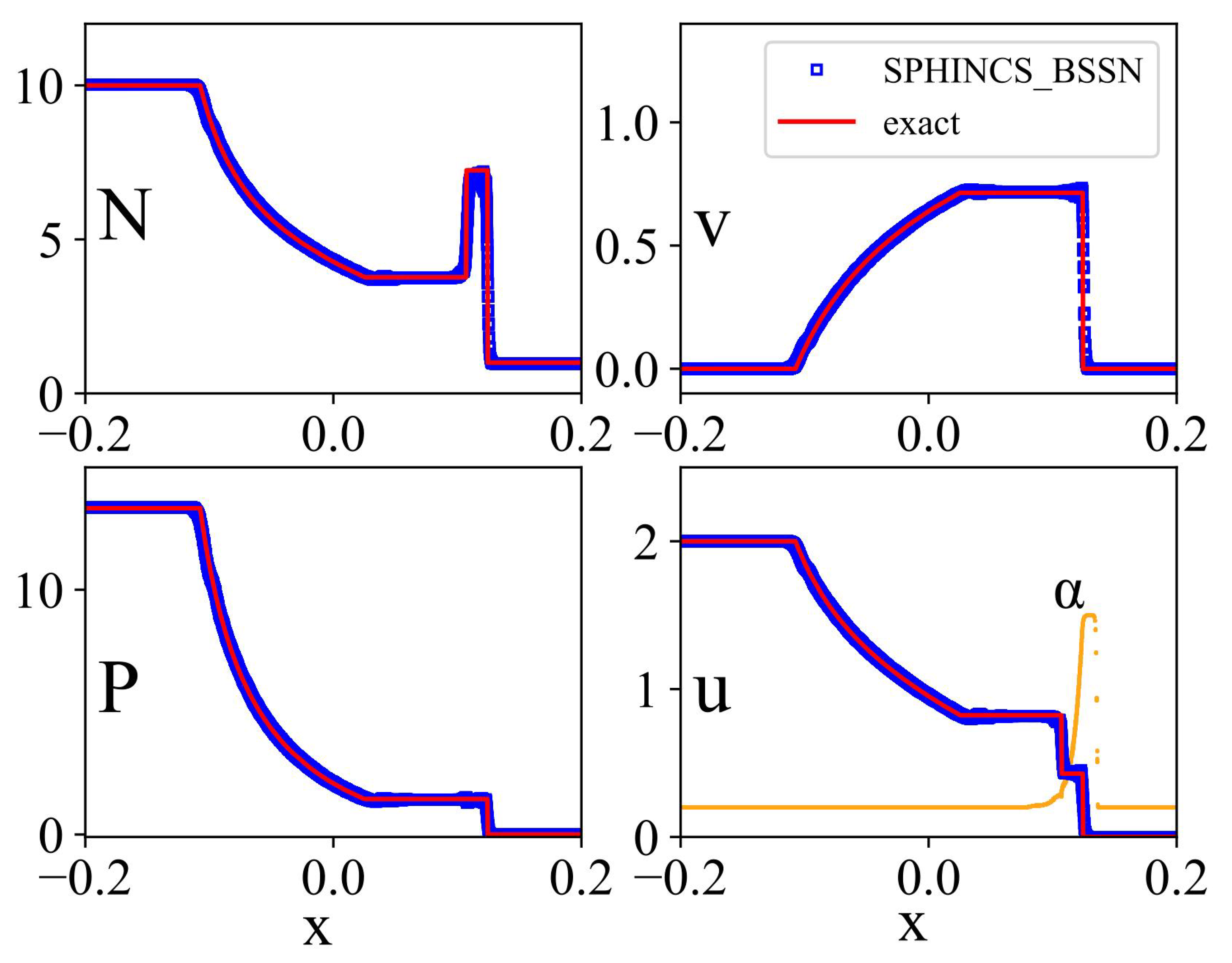
3.1. Shock Tube
3.2. Binary Mergers
3.2.1. Performed Simulations
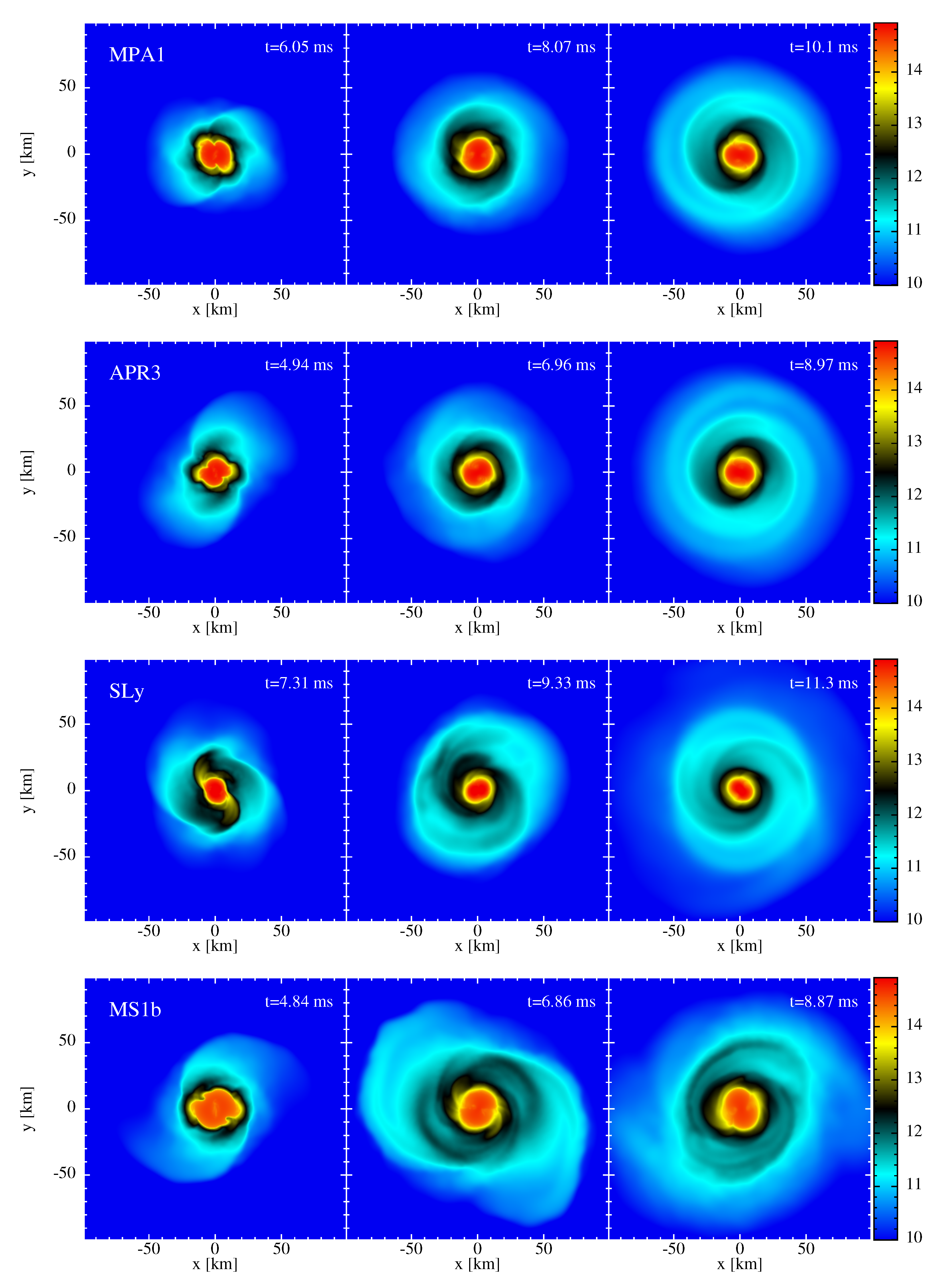
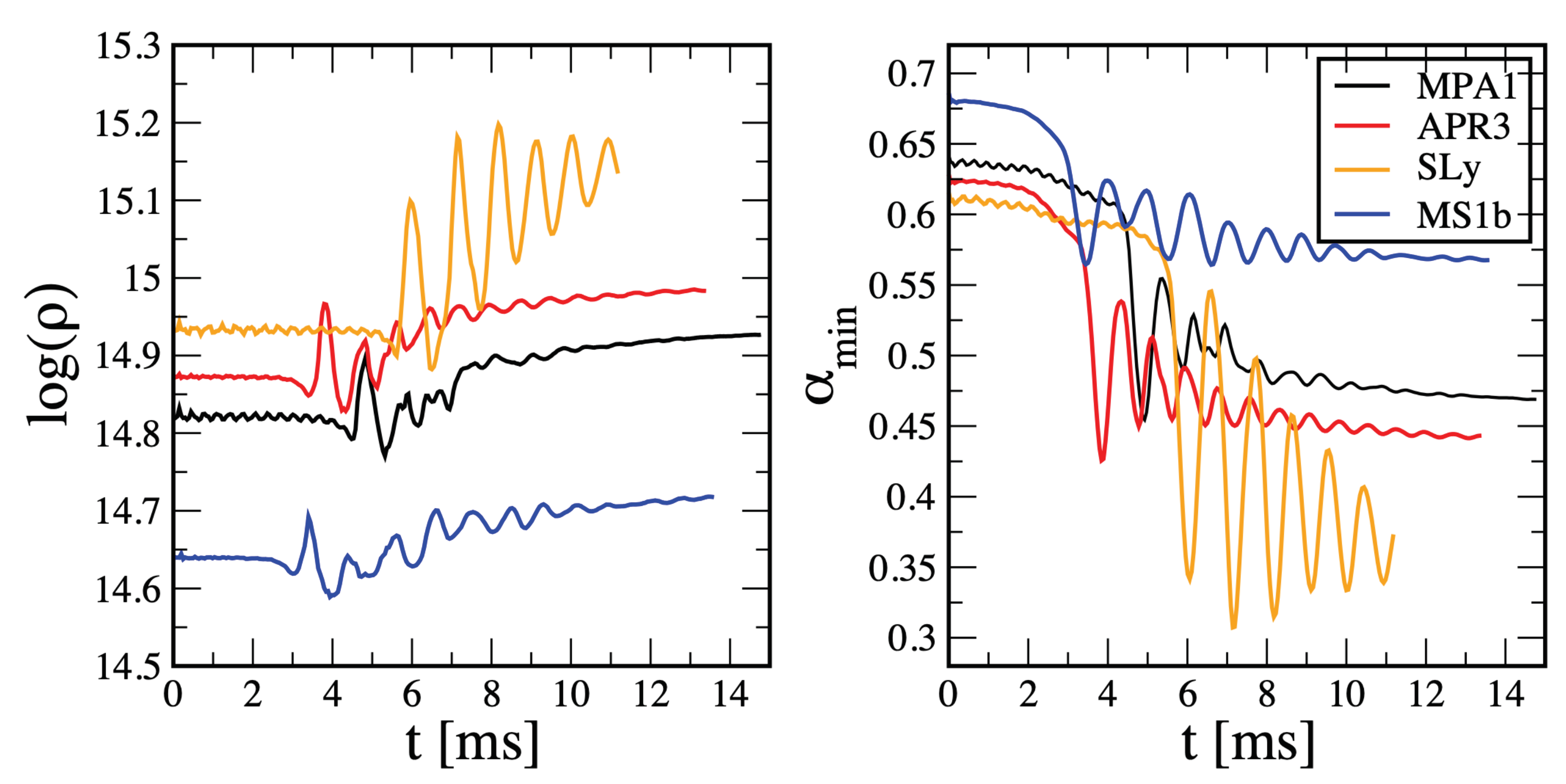
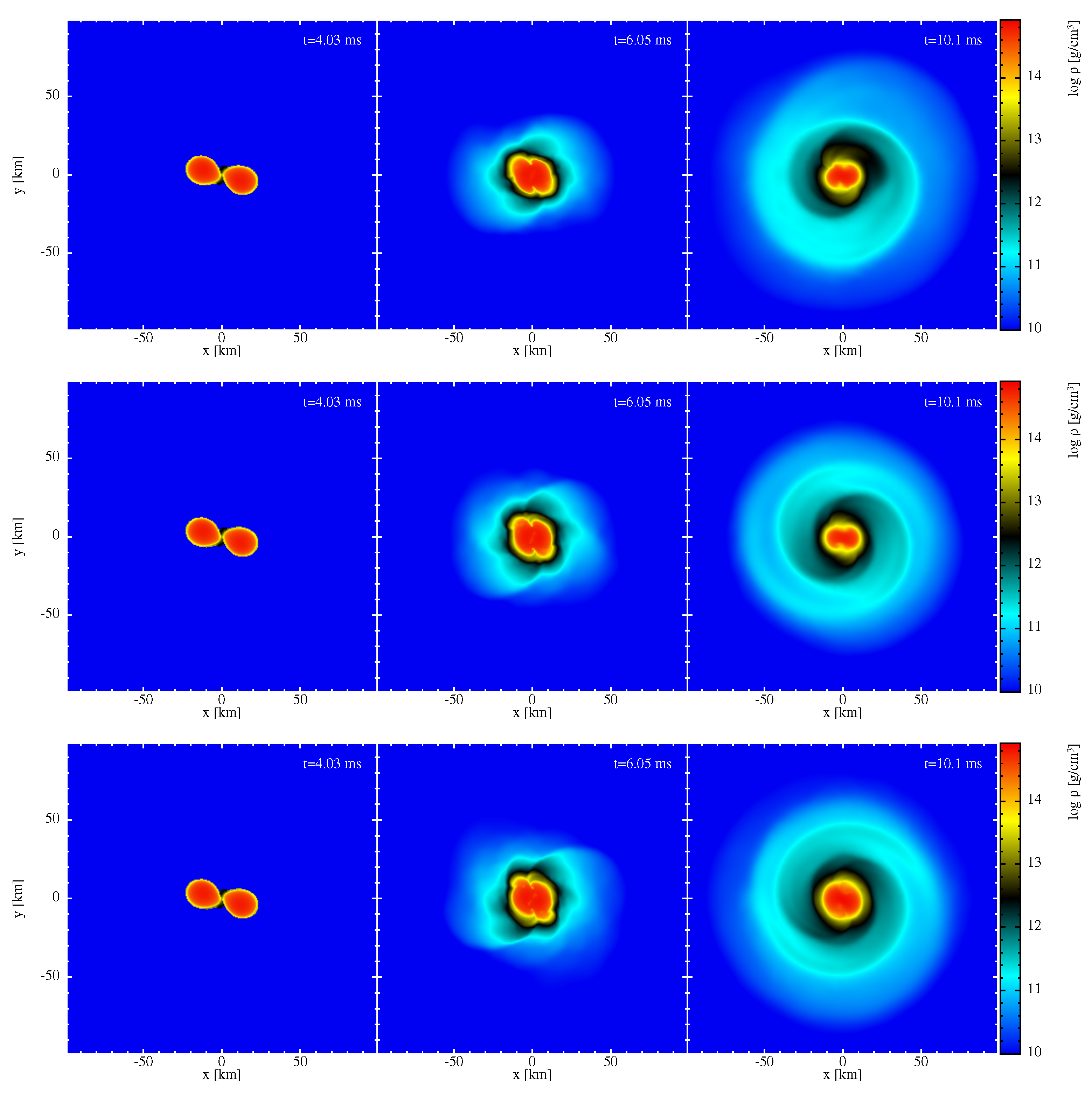
3.2.2. Dynamical Evolution
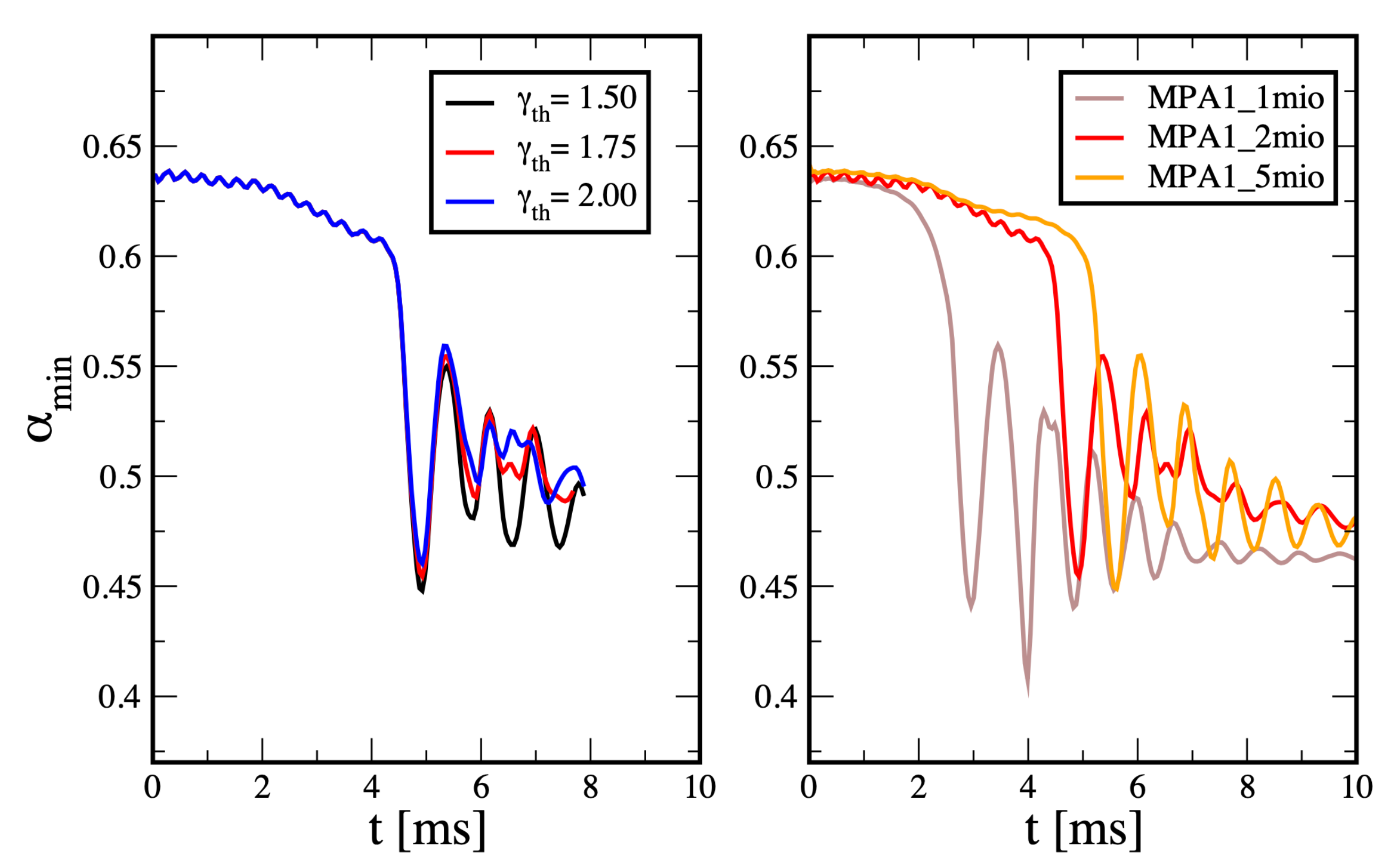
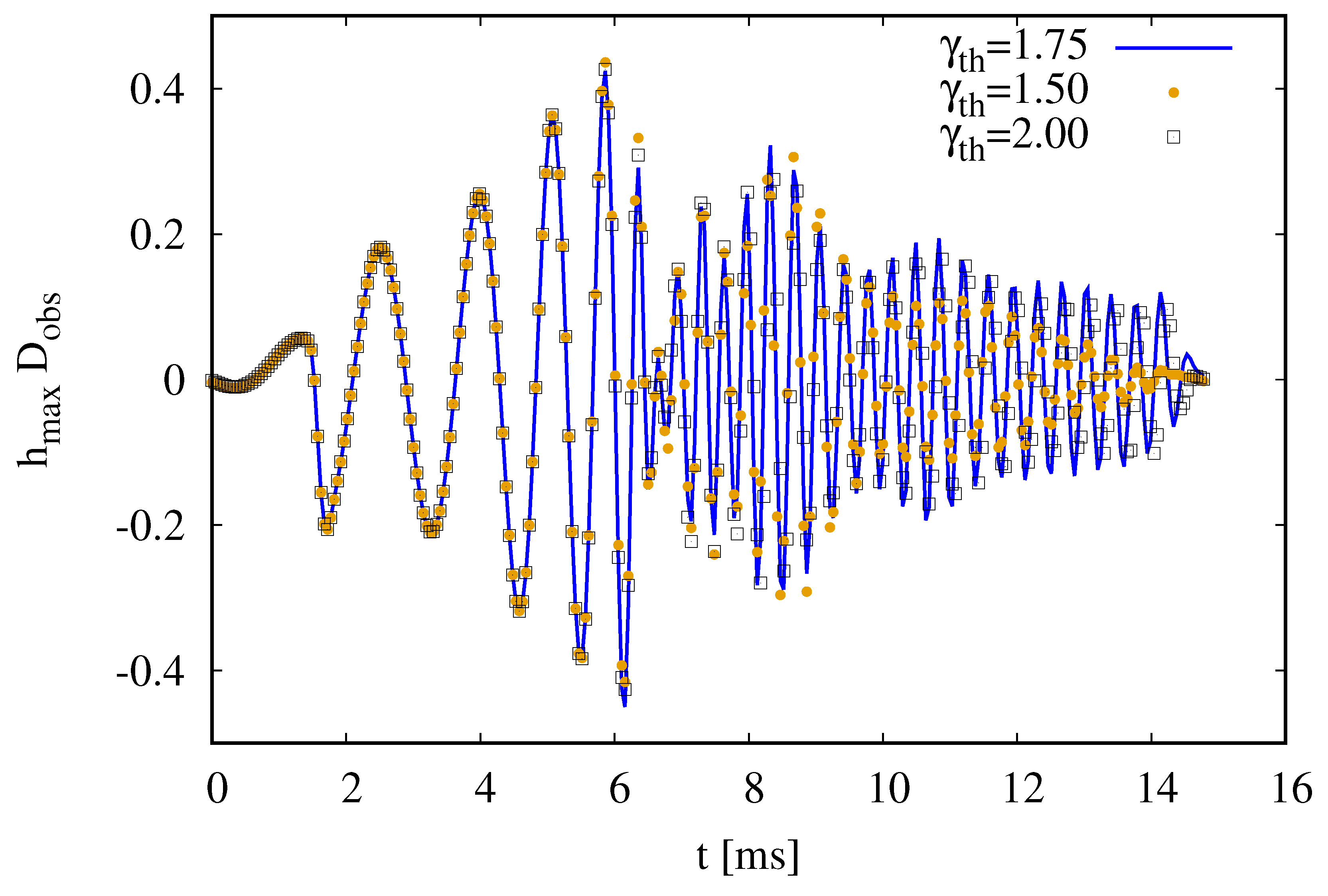
3.2.3. Impact of the Thermal Index
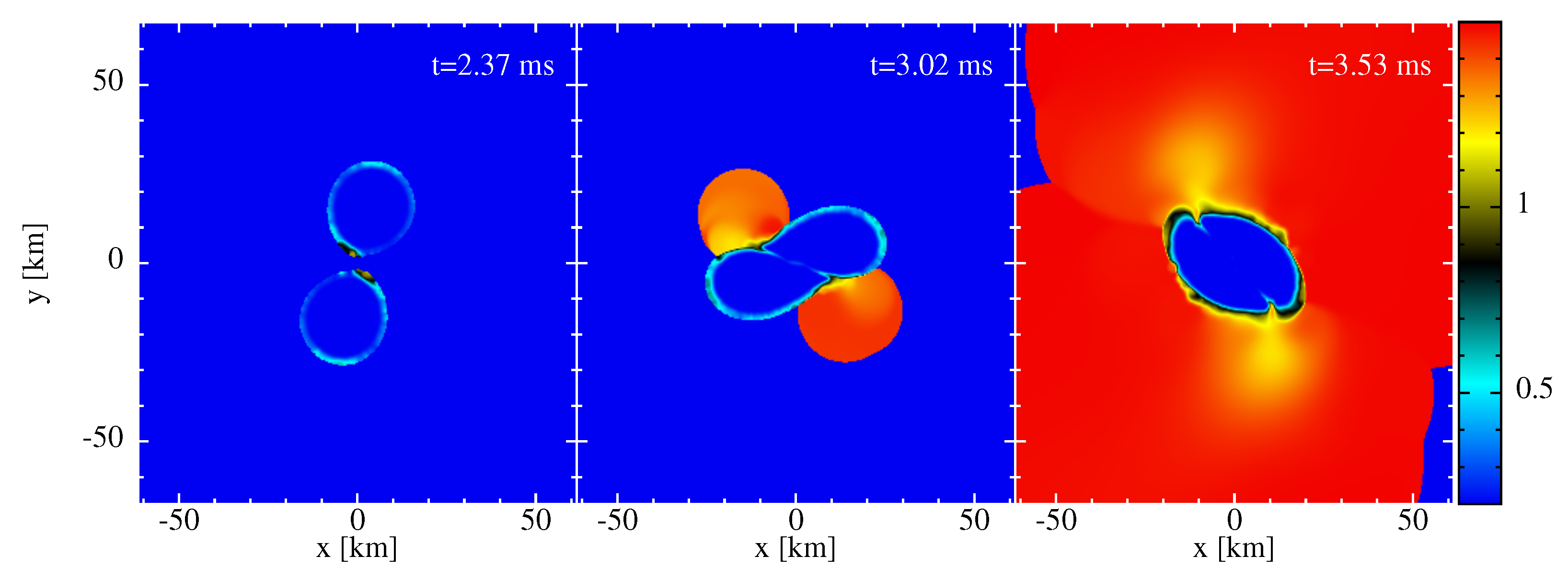
3.2.4. The Triggering of Artificial Dissipation
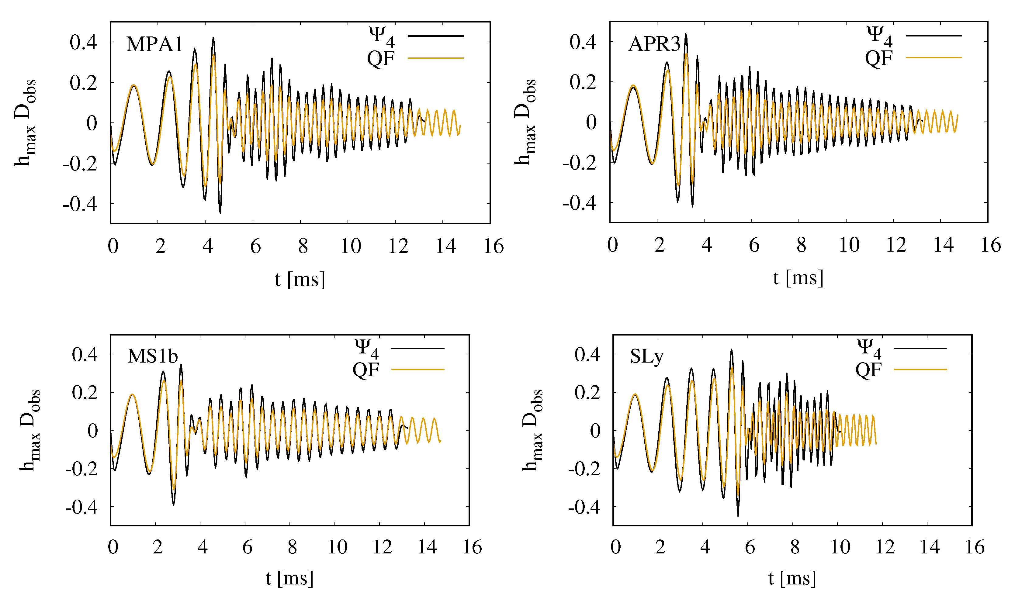
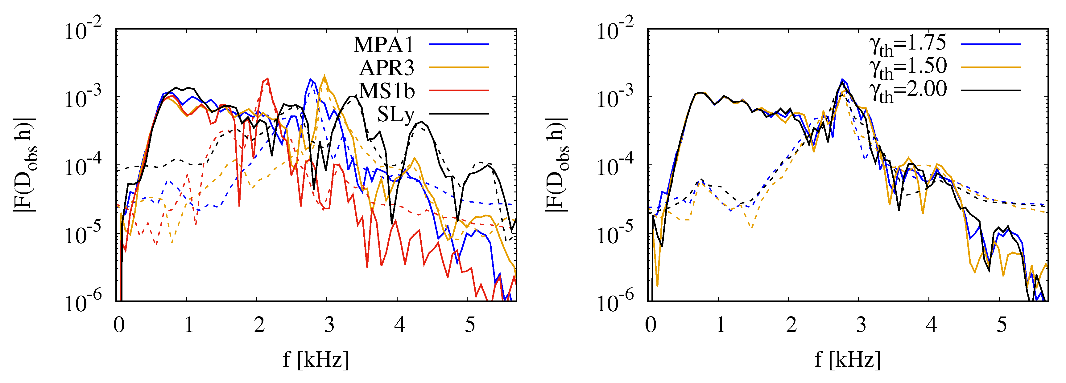
3.2.5. Gravitational Wave Emission
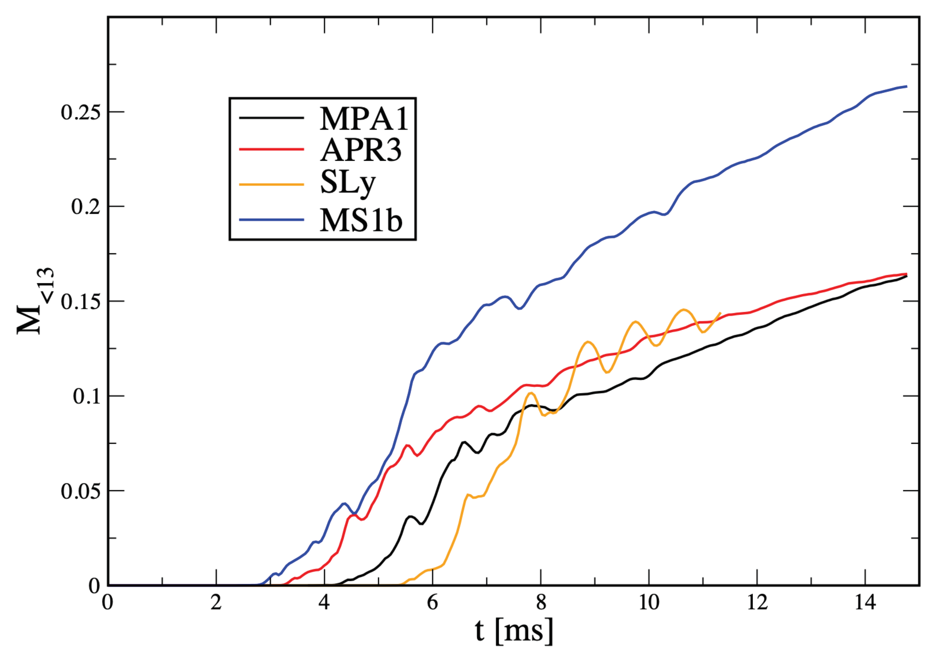
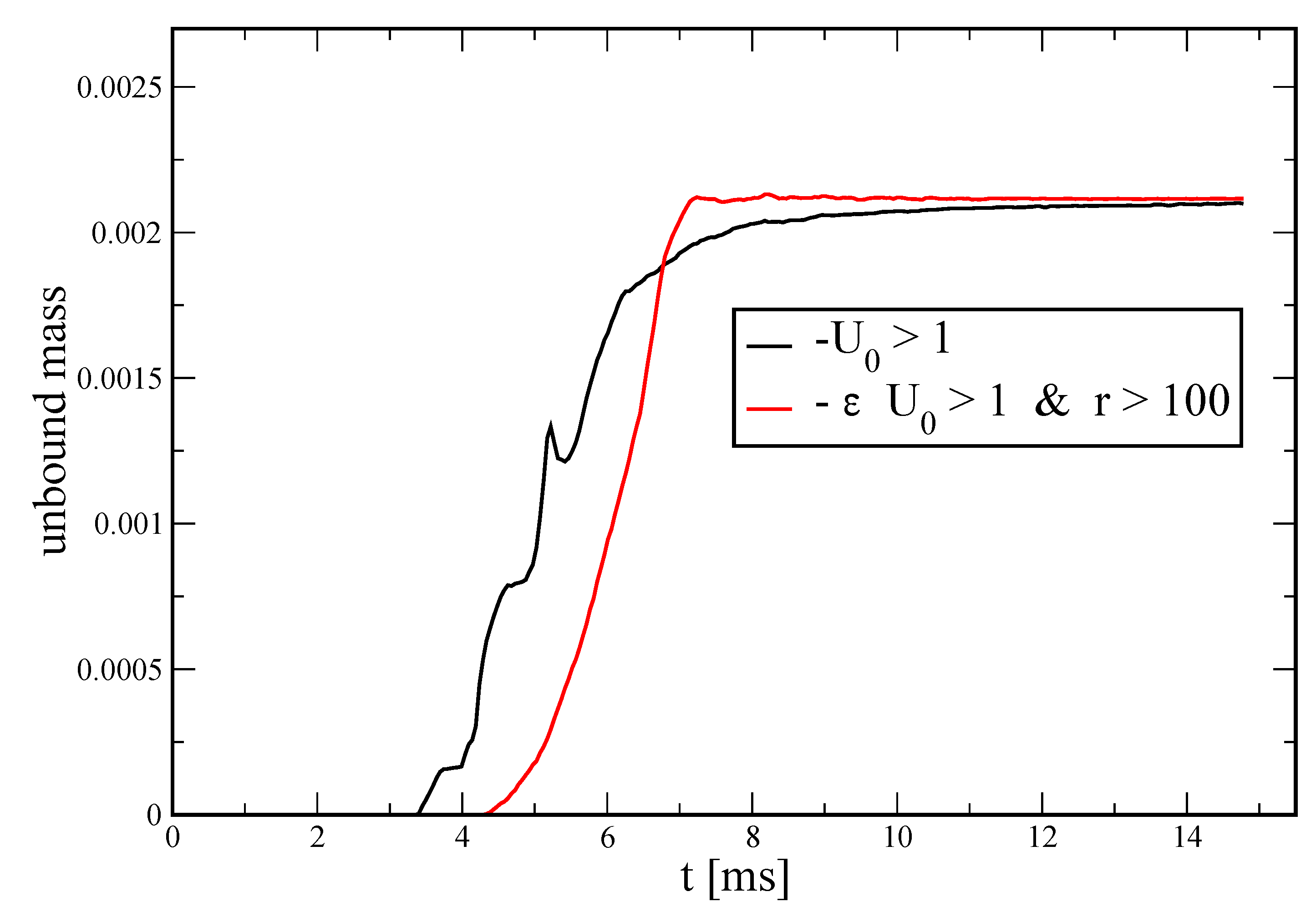
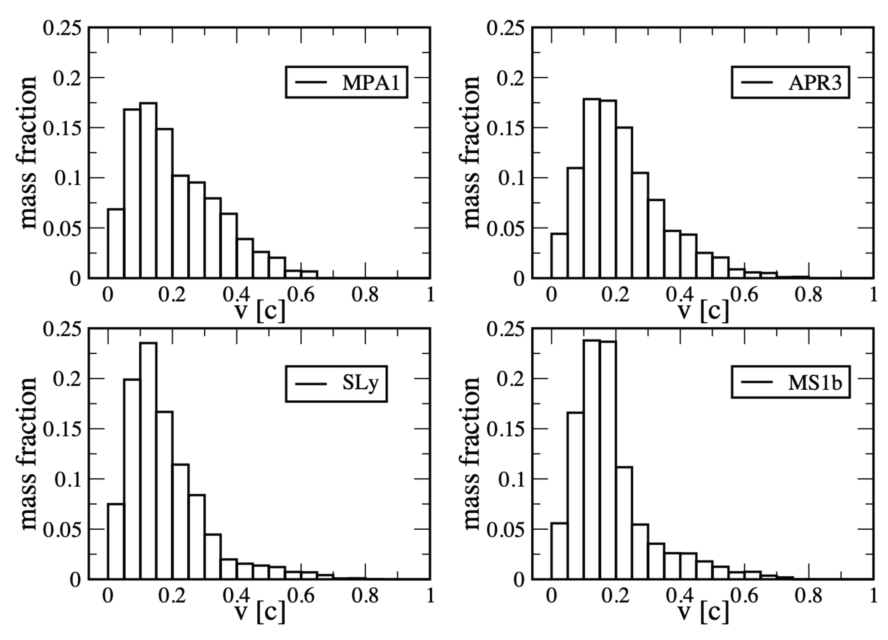
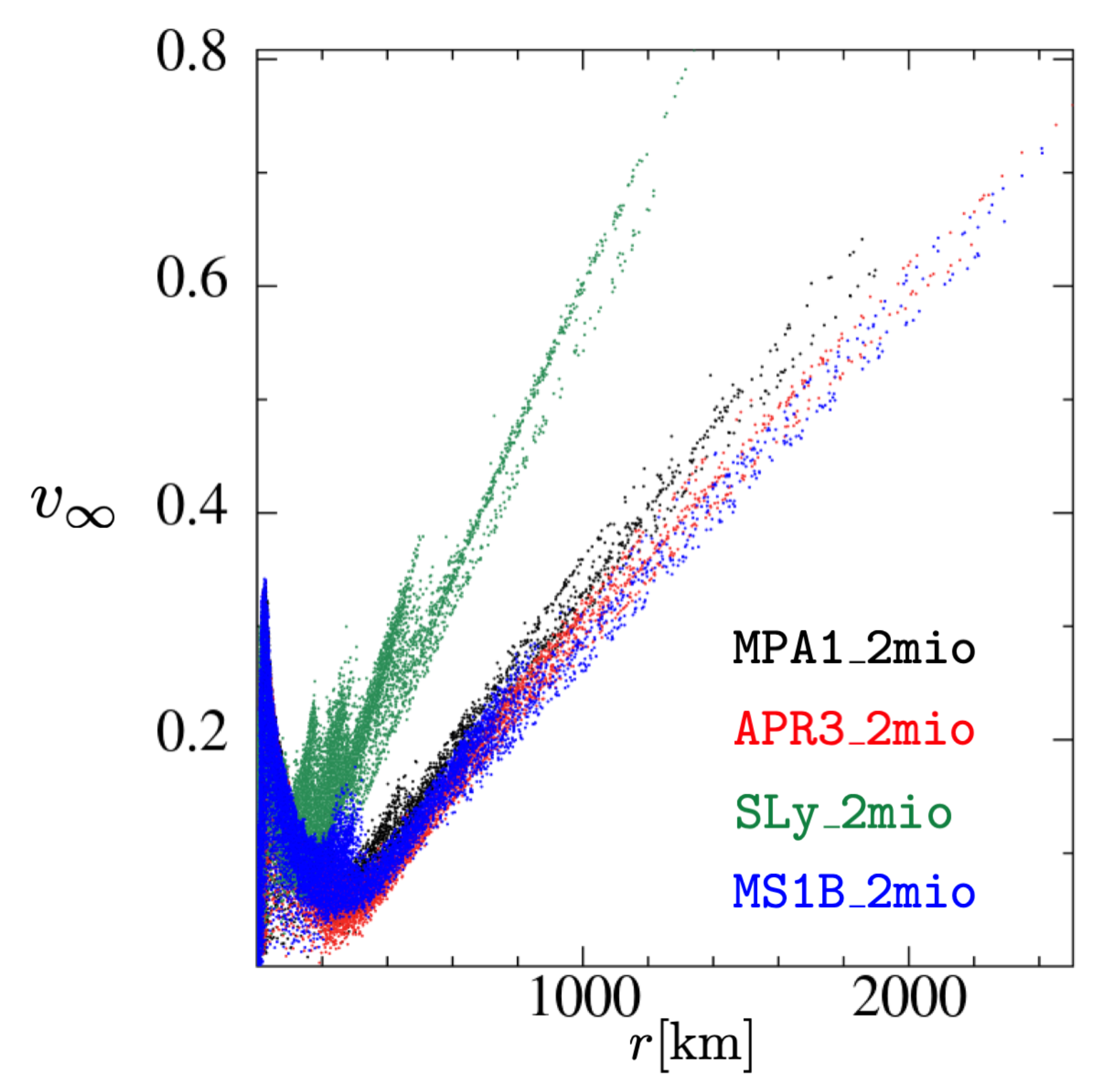
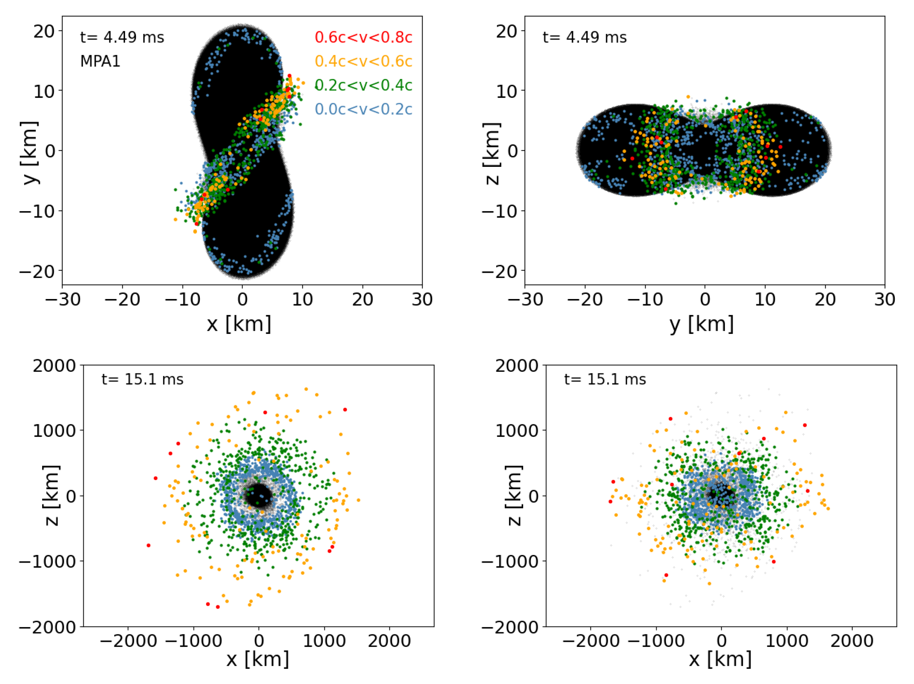
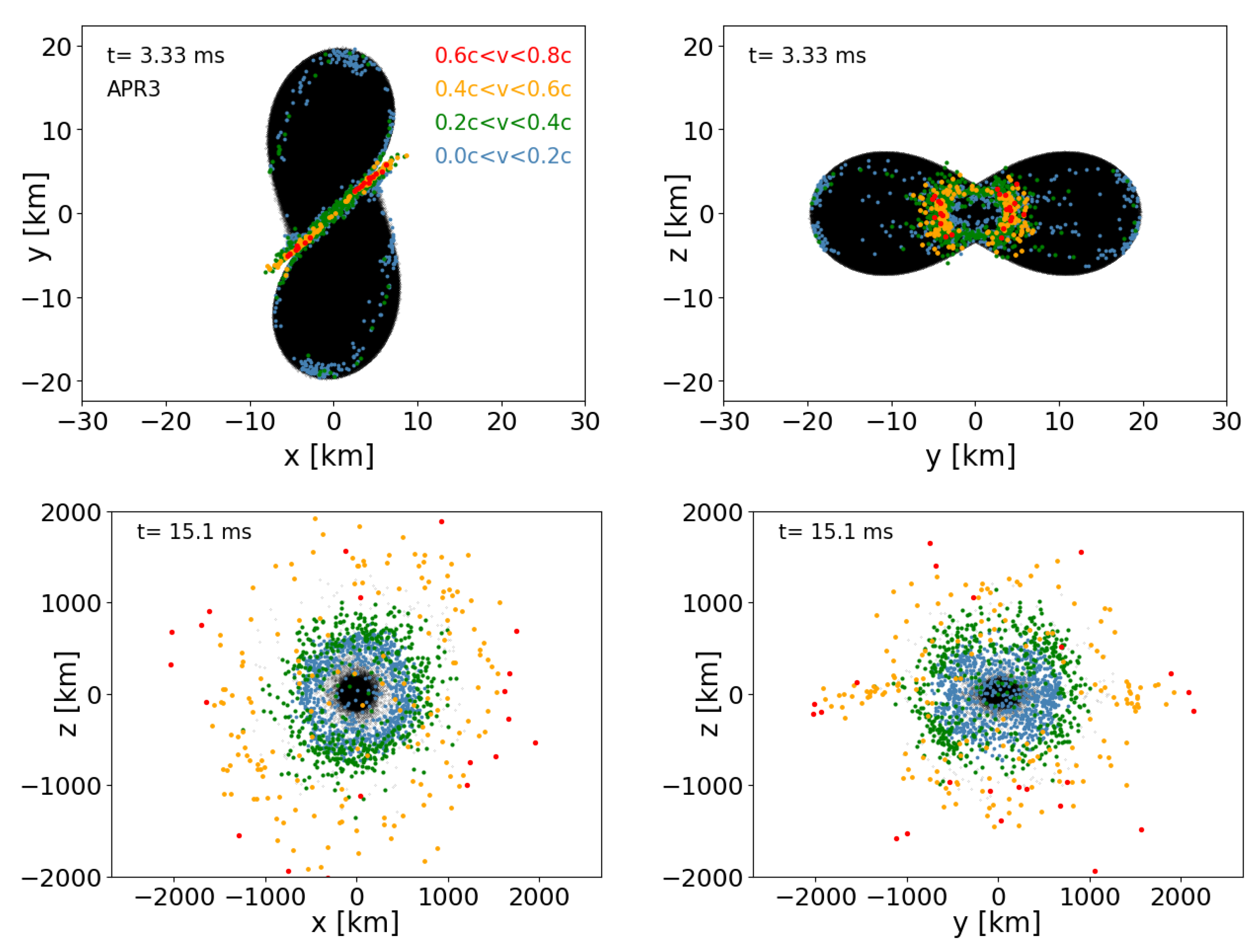
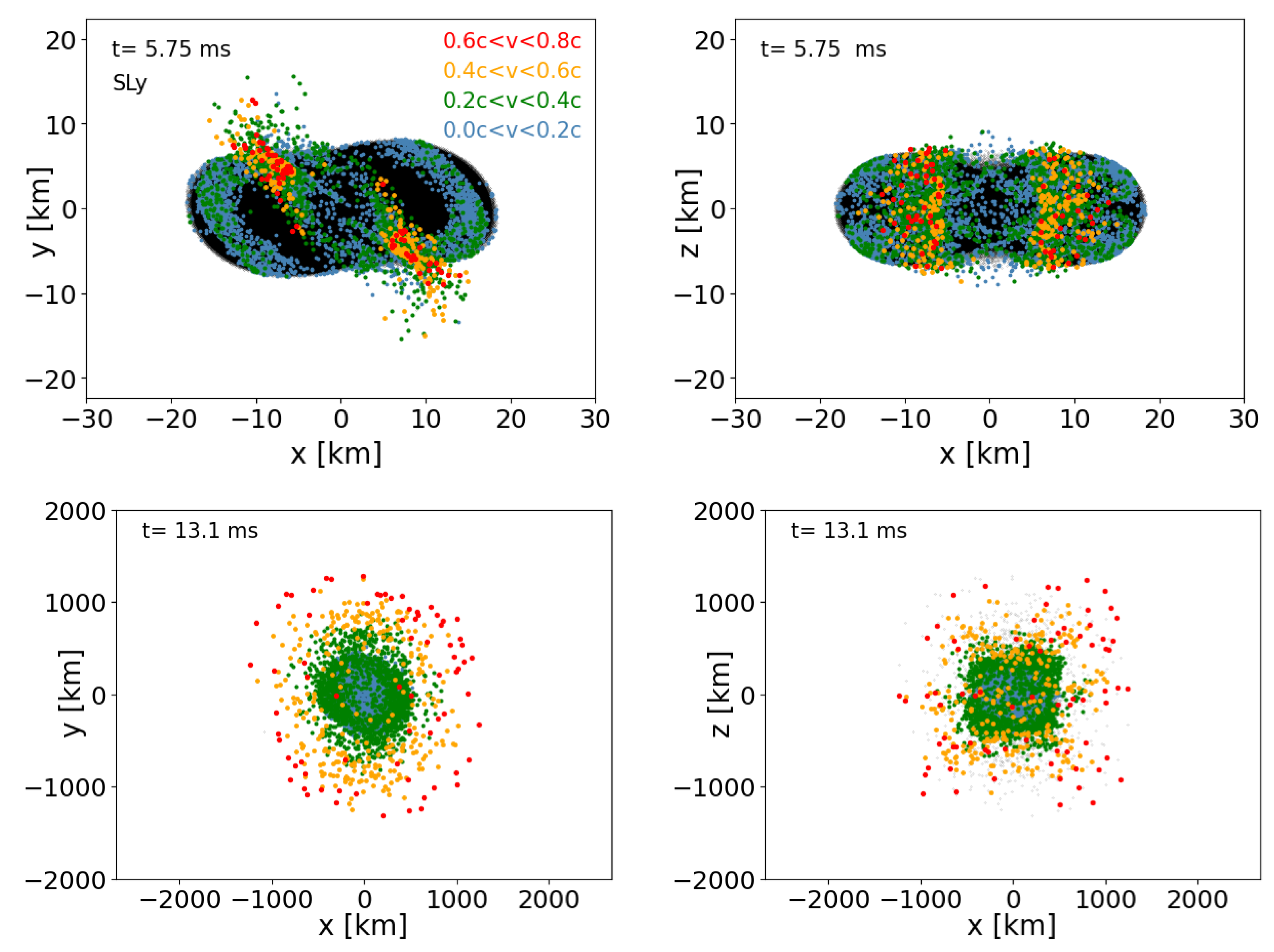
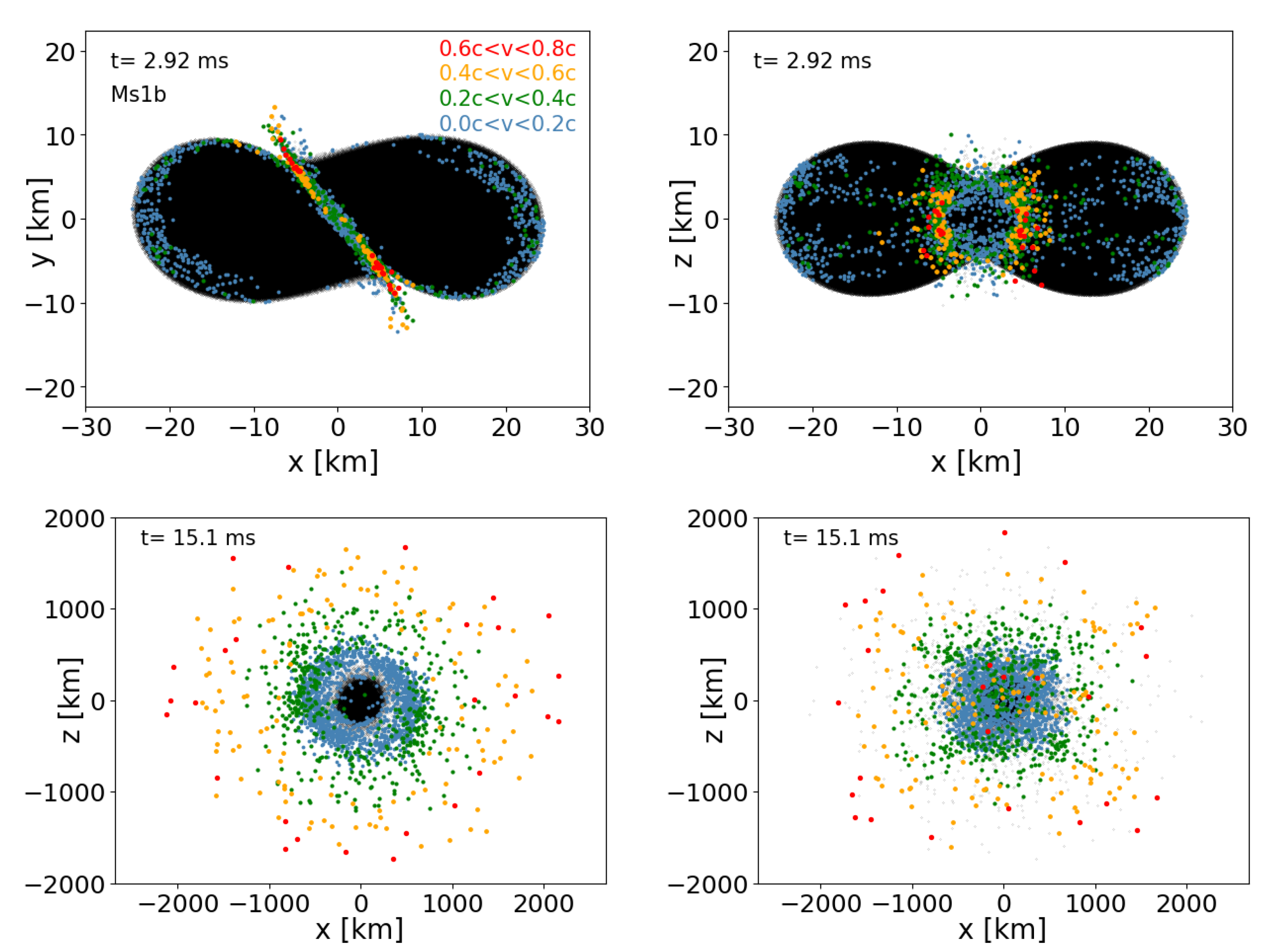
3.2.6. Ejecta
4. Summary
Author Contributions
Funding
Institutional Review Board Statement
Informed Consent Statement
Data Availability Statement
Acknowledgments
Conflicts of Interest
Abbreviations
| ADM | Arnowitt–Deser–Misner |
| BH | Black Hole |
| BSSN | formulation according to Baumgarte, Shapiro, Shibata, and Nakamura |
| EOS | Equation Of State |
| GR | General Relativity |
| GW | Gravitational Wave |
| SPH | Smooth Particle Hydrodynamics |
| SPHINCS | Smooth Particle Hydrodynamics in Curved Spacetime |
Appendix A. Recovery Procedure for Piecewise Polytropic Equations of State
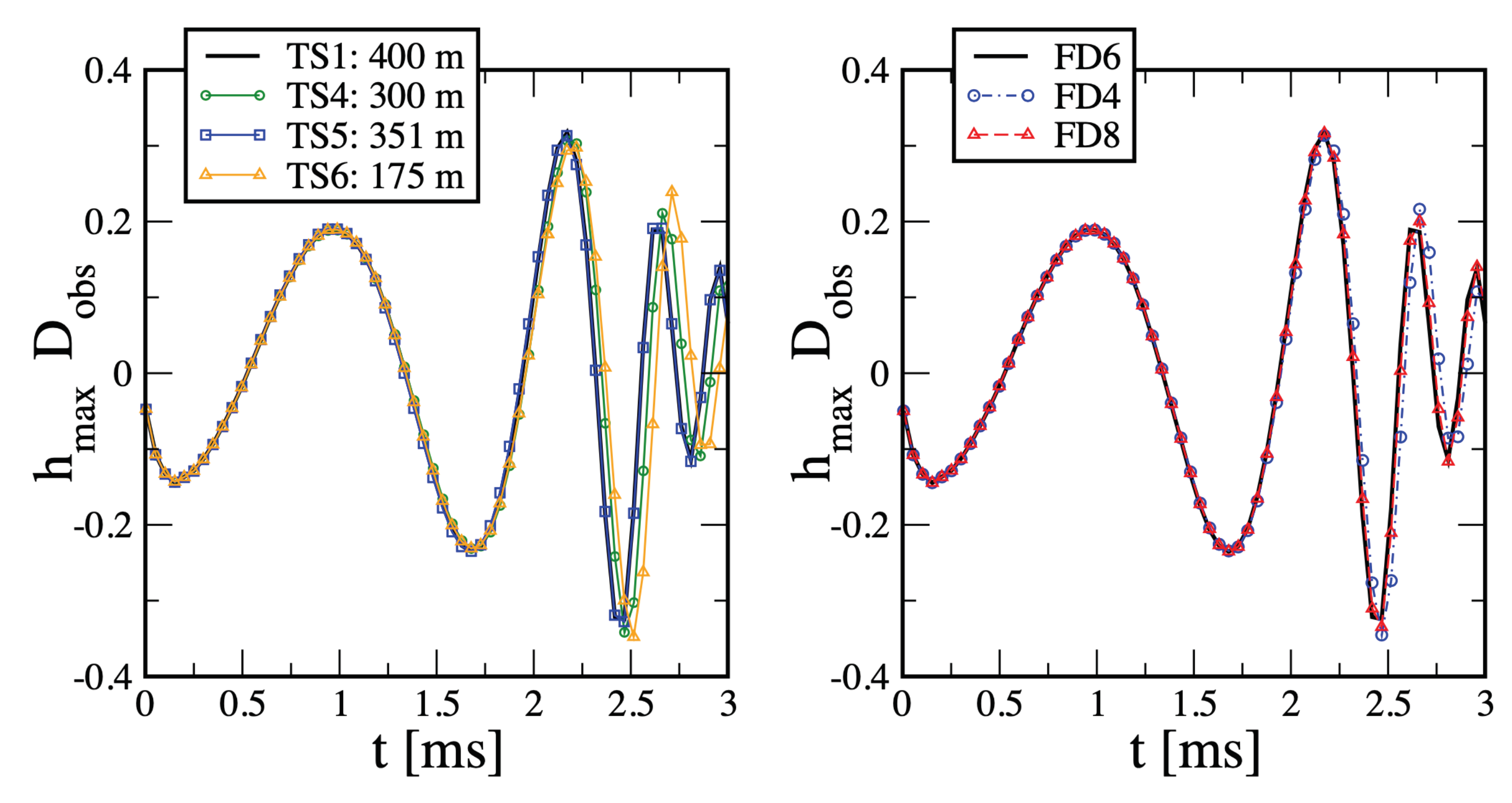
Appendix B. Which Resolution?
- TS1: the outer boundary in each coordinate direction is located at 375 (≈554 km), five refinement levels and grid points which corresponds to the finest grid resolution length of m. We use here our default, i.e., 6th order, Finite Differencing (“FD6”).
- TS2: same as TS1, but FD4
- TS3: same as TS1, but FD8
- TS4: same as TS1, but grid points, i.e., m
- TS5: same as TS1, but grid points, i.e., m.
- TS6: same as TS1, but grid points, i.e., m.

References
- Abbott, R.; Abbott, T.D.; Abraham, S.; Acernese, F.; Ackley, K.; Adams, A.; Adams, C.; Adhikari, R.X.; Adya, V.B.; Affeldt, C.; et al. GWTC-2: Compact Binary Coalescences Observed by LIGO and Virgo during the First Half of the Third Observing Run. Phys. Rev. X 2021, 11, 021053. [Google Scholar] [CrossRef]
- Baiotti, L. Gravitational waves from neutron star mergers and their relation to the nuclear equation of state. Prog. Part. Nucl. Phys. 2019, 109, 103714. [Google Scholar] [CrossRef]
- Ruffert, M.; Janka, H.; Takahashi, K.; Schaefer, G. Coalescing neutron stars-a step towards physical models. II. Neutrino emission, neutron tori, and gamma-ray bursts. Astron. Astrophys. 1997, 319, 122–153. [Google Scholar]
- Rosswog, S.; Liebendörfer, M. High-resolution calculations of merging neutron stars—II. Neutrino emission. Mon. Not. R. Astron. Soc. 2003, 342, 673–689. [Google Scholar] [CrossRef]
- Sekiguchi, Y.; Kiuchi, K.; Kyutoku, K.; Shibata, M. Gravitational Waves and Neutrino Emission from the Merger of Binary Neutron Stars. Phys. Rev. Lett. 2011, 107, 051102. [Google Scholar] [CrossRef]
- Perego, A.; Rosswog, S.; Cabezón, R.M.; Korobkin, O.; Käppeli, R.; Arcones, A.; Liebendörfer, M. Neutrino-driven winds from neutron star merger remnants. Mon. Not. R. Astron. Soc. 2014, 443, 3134–3156. [Google Scholar] [CrossRef]
- Just, O.; Bauswein, A.; Pulpillo, R.A.; Goriely, S.; Janka, H.T. Comprehensive nucleosynthesis analysis for ejecta of compact binary mergers. Mon. Not. R. Astron. Soc. 2015, 448, 541–567. [Google Scholar] [CrossRef]
- Fujibayashi, S.; Shibata, M.; Wanajo, S.; Kiuchi, K.; Kyutoku, K.; Sekiguchi, Y. Mass ejection from disks surrounding a low-mass black hole: Viscous neutrino-radiation hydrodynamics simulation in full general relativity. Phys. Rev. D 2020, 101, 083029. [Google Scholar] [CrossRef]
- Foucart, F.; Duez, M.D.; Hébert, F.; Kidder, L.E.; Kovarik, P.; Pfeiffer, H.P.; Scheel, M.A. Implementation of Monte Carlo Transport in the General Relativistic SpEC Code. Astrophys. J. 2021, 920, 82. [Google Scholar] [CrossRef]
- Just, O.; Goriely, S.; Janka, H.T.; Nagataki, S.; Bauswein, A. Neutrino absorption and other physics dependencies in neutrino-cooled black hole accretion discs. Mon. Not. R. Astron. Soc. 2022, 509, 1377–1412. [Google Scholar] [CrossRef]
- Radice, D.; Bernuzzi, S.; Perego, A.; Haas, R. A New Moment-Based General-Relativistic Neutrino-Radiation Transport Code: Methods and First Applications to Neutron Star Mergers. Mon. Not. R. Astron. Soc. 2022, 512, 1499–1521. [Google Scholar] [CrossRef]
- Price, D.; Rosswog, S. Producing ultra-strong magnetic fields in neutron star mergers. Science 2006, 312, 719. [Google Scholar] [CrossRef] [PubMed]
- Kiuchi, K.; Cerdá-Durán, P.; Kyutoku, K.; Sekiguchi, Y.; Shibata, M. Efficient magnetic-field amplification due to the Kelvin-Helmholtz instability in binary neutron star mergers. Phys. Rev. D 2015, 92, 124034. [Google Scholar] [CrossRef]
- Palenzuela, C.; Liebling, S.L.; Neilsen, D.; Lehner, L.; Caballero, O.L.; O’Connor, E.; Anderson, M. Effects of the microphysical equation of state in the mergers of magnetized neutron stars with neutrino cooling. Phys. Rev. D 2015, 92, 044045. [Google Scholar] [CrossRef]
- Rosswog, S.; Diener, P. SPHINCS_BSSN: A general relativistic smooth particle hydrodynamics code for dynamical spacetimes. Class. Quantum Gravity 2021, 38, 115002. [Google Scholar] [CrossRef]
- Diener, P.; Rosswog, S.; Torsello, F. SimuLating neutron star mergers with the Lagrangian Numerical Relativity code SPHINCS_BSSN. Eur. Phys. J. A 2022, 58, 74. [Google Scholar] [CrossRef]
- Shibata, M.; Nakamura, T. Evolution of three-dimensional gravitational waves: Harmonic slicing case. Phys. Rev. D 1995, 52, 5428–5444. [Google Scholar] [CrossRef]
- Baumgarte, T.W.; Shapiro, S.L. Numerical integration of Einstein’s field equations. Phys. Rev. D 1999, 59, 024007. [Google Scholar] [CrossRef]
- Rosswog, S.; Liebendörfer, M.; Thielemann, F.K.; Davies, M.; Benz, W.; Piran, T. Mass ejection in neutron star mergers. Astron. Astrophys. 1999, 341, 499–526. [Google Scholar]
- Oechslin, R.; Janka, H. Gravitational Waves from Relativistic Neutron-Star Mergers with Microphysical Equations of State. Phys. Rev. Lett. 2007, 99, 121102. [Google Scholar] [CrossRef]
- Bauswein, A.; Goriely, S.; Janka, H.T. Systematics of Dynamical Mass Ejection, Nucleosynthesis, and Radioactively Powered Electromagnetic Signals from Neutron-star Mergers. Astrophys. J. 2013, 773, 78. [Google Scholar] [CrossRef]
- Hotokezaka, K.; Kiuchi, K.; Kyutoku, K.; Okawa, H.; Sekiguchi, Y.i.; Shibata, M.; Taniguchi, K. Mass ejection from the merger of binary neutron stars. Phys. Rev. D 2013, 87, 024001. [Google Scholar] [CrossRef]
- Radice, D.; Perego, A.; Hotokezaka, K.; Fromm, S.A.; Bernuzzi, S.; Roberts, L.F. Binary Neutron Star Mergers: Mass Ejection, Electromagnetic Counterparts, and Nucleosynthesis. Astrophys. J. 2018, 869, 130. [Google Scholar] [CrossRef]
- Schoepe, A.; Hilditch, D.; Bugner, M. Revisiting hyperbolicity of relativistic fluids. Phys. Rev. D 2018, 97, 123009. [Google Scholar] [CrossRef]
- Rosswog, S. The Lagrangian hydrodynamics code MAGMA2. Mon. Not. R. Astron. Soc. 2020, 498, 4230–4255. [Google Scholar] [CrossRef]
- LORENE Library. Available online: https://lorene.obspm.fr (accessed on 1 May 2022).
- Read, J.S.; Lackey, B.D.; Owen, B.J.; Friedman, J.L. Constraints on a phenomenologically parametrized neutron-star equation of state. Phys. Rev. D 2009, 79, 124032. [Google Scholar] [CrossRef]
- Cullen, L.; Dehnen, W. Inviscid smoothed particle hydrodynamics. Mon. Not. R. Astron. Soc. 2010, 408, 669–683. [Google Scholar] [CrossRef]
- Rosswog, S. Boosting the accuracy of SPH techniques: Newtonian and special-relativistic tests. Mon. Not. R. Astron. Soc. 2015, 448, 3628–3664. [Google Scholar] [CrossRef]
- Rosswog, S. Astrophysical Smooth Particle Hydrodynamics. New Astron. Rev. 2009, 53, 78–104. [Google Scholar] [CrossRef]
- Rosswog, S. A Simple, Entropy-based Dissipation Trigger for SPH. Astrophys. J. 2020, 898, 60. [Google Scholar] [CrossRef]
- Alcubierre, M. Introduction to 3+1 Numerical Relativity; Oxford University Press: Oxford, UK, 2008. [Google Scholar]
- Baumgarte, T.W.; Shapiro, S.L. Numerical Relativity: Solving Einstein’s Equations on the Computer; Cambridge University Press: Cambridge, UK, 2010. [Google Scholar]
- Rezzolla, L.; Zanotti, O. Relativistic Hydrodynamics; Oxford University Press: Oxford, UK, 2013. [Google Scholar]
- Shibata, M. Numerical Relativity; World Scientific: Singapore, 2016. [Google Scholar] [CrossRef]
- Wendland, H. Piecewise polynomial, positive definite and compactly supported radial functions of minimal degree. Adv. Comput. Math. 1995, 4, 389–396. [Google Scholar] [CrossRef]
- Gafton, E.; Rosswog, S. A fast recursive coordinate bisection tree for neighbour search and gravity. Mon. Not. R. Astron. Soc. 2011, 418, 770–781. [Google Scholar] [CrossRef]
- Laguna, P.; Miller, W.A.; Zurek, W.H. Smoothed particle hydrodynamics near a black hole. Astrophys. J. 1993, 404, 678–685. [Google Scholar] [CrossRef]
- von Neumann, J.; Richtmyer, R.D. A Method for the Numerical Calculation of Hydrodynamic Shocks. J. Appl. Phys. 1950, 21, 232–237. [Google Scholar] [CrossRef]
- Liptai, D.; Price, D.J. General relativistic smoothed particle hydrodynamics. Mon. Not. R. Astron. Soc. 2019, 485, 819–842. [Google Scholar] [CrossRef]
- Christensen, R.B. Godunov Methods on a Staggered Mesh—An Improved Artificial Viscosity. In Nuclear Explosives Code Developers Conference; Lawrence Livermore National Lab, Lawrence Livermore Technical Report; 1990; Volume UCRL-JC-105269. Available online: https://ntrl.ntis.gov/NTRL/dashboard/searchResults/titleDetail/DE92011973.xhtml (accessed on 1 May 2022).
- Frontiere, N.; Raskin, C.D.; Owen, J.M. CRKSPH—A Conservative Reproducing Kernel Smoothed Particle Hydrodynamics Scheme. J. Comput. Phys. 2017, 332, 160–209. [Google Scholar] [CrossRef]
- Brown, J.D.; Diener, P.; Sarbach, O.; Schnetter, E.; Tiglio, M. Turduckening black holes: An analytical and computational study. Phys. Rev. D 2009, 79, 044023. [Google Scholar] [CrossRef]
- Einstein Toolkit Web Page. 2020. Available online: https://einsteintoolkit.org/ (accessed on 9 December 2020).
- Löffler, F.; Faber, J.; Bentivegna, E.; Bode, T.; Diener, P.; Haas, R.; Hinder, I.; Mundim, B.C.; Ott, C.D.; Schnetter, E.; et al. The Einstein Toolkit: A Community Computational Infrastructure for Relativistic Astrophysics. Class. Quantum Grav. 2012, 29, 115001. [Google Scholar] [CrossRef]
- Cottet, G.H.; Koumoutsakos, P.D. Vortex Methods; Cambridge University Press: Cambridge, UK, 2000. [Google Scholar]
- Cottet, G.; Etancelin, J.; Perignon, F.; Picard, C. High order Semi-Lagrangian particle methods for tranport equations. ESAIM Math. Model. Numer. Anal. Edp Sci. 2014, 48, 1029–1060. [Google Scholar] [CrossRef]
- Douchin, F.; Haensel, P. A unified equation of state of dense matter and neutron star structure. Astron. Astrophys. 2001, 380, 151–167. [Google Scholar] [CrossRef]
- Akmal, A.; Pandharipande, V.R.; Ravenhall, D.G. Equation of state of nucleon matter and neutron star structure. Phys. Rev. C 1998, 58, 1804–1828. [Google Scholar] [CrossRef]
- Müther, H.; Prakash, M.; Ainsworth, T.L. The nuclear symmetry energy in relativistic Brueckner-Hartree-Fock calculations. Phys. Lett. B 1987, 199, 469–474. [Google Scholar] [CrossRef]
- Müller, H.; Serot, B.D. Relativistic mean-field theory and the high-density nuclear equation of state. Nuc. Phys. A 1996, 606, 508–537. [Google Scholar] [CrossRef]
- Pacilio, C.; Maselli, A.; Fasano, M.; Pani, P. Ranking Love Numbers for the Neutron Star Equation of State: The Need for Third-Generation Detectors. Phys. Rev. Lett. 2022, 128, 101101. [Google Scholar] [CrossRef] [PubMed]
- Cromartie, H.T.; Fonseca, E.; Ransom, S.M.; Demorest, P.B.; Arzoumanian, Z.; Blumer, H.; Brook, P.R.; DeCesar, M.E.; Dolch, T.; Ellis, J.A.; et al. Relativistic Shapiro delay measurements of an extremely massive millisecond pulsar. Nat. Astron. 2020, 4, 72–76. [Google Scholar] [CrossRef]
- Fryer, C.L.; Belczynski, K.; Ramirez-Ruiz, E.; Rosswog, S.; Shen, G.; Steiner, A.W. The Fate of the Compact Remnant in Neutron Star Mergers. Astrophys. J. 2015, 812, 24. [Google Scholar] [CrossRef]
- Margalit, B.; Metzger, B.D. Constraining the Maximum Mass of Neutron Stars from Multi-messenger Observations of GW170817. Astrophys. J. 2017, 850, L19. [Google Scholar] [CrossRef]
- Bauswein, A.; Just, O.; Janka, H.T.; Stergioulas, N. Neutron-star Radius Constraints from GW170817 and Future Detections. Astrophys. J. 2017, 850, L34. [Google Scholar] [CrossRef]
- Shibata, M.; Fujibayashi, S.; Hotokezaka, K.; Kiuchi, K.; Kyutoku, K.; Sekiguchi, Y.; Tanaka, M. Modeling GW170817 based on numerical relativity and its implications. Phys. Rev. D 2017, 96, 123012. [Google Scholar] [CrossRef]
- Rezzolla, L.; Most, E.R.; Weih, L.R. Using Gravitational-wave Observations and Quasi-universal Relations to Constrain the Maximum Mass of Neutron Stars. Astrophys. J. 2018, 852, L25. [Google Scholar] [CrossRef]
- Biswas, B.; Datta, S. Constraining neutron star properties with a new equation of state insensitive approach. arXiv 2021, arXiv:2112.10824. [Google Scholar]
- Rhoades, C.E.; Ruffini, R. Maximum Mass of a Neutron Star. Phys. Rev. Lett. 1974, 32, 324–327. [Google Scholar] [CrossRef]
- Kalogera, V.; Baym, G. The Maximum Mass of a Neutron Star. Astrophys. J. 1996, 470, L61. [Google Scholar] [CrossRef]
- Schaffner-Bielich, J. Compact Stars, 1st ed.; Cambridge University Press: Cambridge, UK, 2020. [Google Scholar]
- Abbott, B.P.; Abbott, R.; Abbott, T.D.; Acernese, F.; Ackley, K.; Adams, C.; Adams, T.; Addesso, P.; Adhikari, R.X.; Adya, V.B.; et al. GW170817: Observation of Gravitational Waves from a Binary Neutron Star Inspiral. Phys. Rev. Lett. 2017, 119, 161101. [Google Scholar] [CrossRef]
- Sod, G. A survey of several finite difference methods for systems of nonlinear hyperbolic conservation laws. J. Comput. Phys. 1978, 43, 1–31. [Google Scholar] [CrossRef]
- Marti, J.; Müller, E. Extension of the Piecewise Parabolic Method to One-Dimensional Relativistic Hydrodynamics. J. Comp. Phys. 1996, 123, 1–14. [Google Scholar] [CrossRef]
- Chow, J.E.; Monaghan, J. Ultrarelativistic SPH. J. Computat. Phys. 1997, 134, 296. [Google Scholar] [CrossRef]
- Siegler, S.; Riffert, H. Smoothed Particle Hydrodynamics Simulations of Ultrarelativistic Shocks with Artificial Viscosity. Astrophys. J. 2000, 531, 1053–1066. [Google Scholar] [CrossRef][Green Version]
- Del Zanna, L.; Bucciantini, N. An efficient shock-capturing central-type scheme for multidimensional relativistic flows. I. Hydrodynamics. Astron. Astrophys. 2002, 390, 1177–1186. [Google Scholar] [CrossRef]
- Marti, J.M.; Müller, E. Numerical Hydrodynamics in Special Relativity. Living Rev. Relativ. 2003, 6, 7. [Google Scholar] [CrossRef]
- Marti, J.M.; Müller, E. Grid-based Methods in Relativistic Hydrodynamics and Magnetohydrodynamics. Living Rev. Comput. Astrophys. 2015, 1, 3. [Google Scholar] [CrossRef]
- Rosswog, S. SPH Methods in the Modelling of Compact Objects. Living Rev. Comput. Astrophys. 2015, 1, 1. [Google Scholar] [CrossRef]
- van Leer, B. Towards the Ultimate Conservative Difference Scheme. IV. A New Approach to Numerical Convection. J. Comput. Phys. 1977, 23, 276. [Google Scholar] [CrossRef]
- Sweby, P.K. High Resolution Schemes Using Flux Limiters for Hyperbolic Conservation Laws. SIAM J. Numer. Anal. 1984, 21, 995–1011. [Google Scholar] [CrossRef]
- Rosswog, S. Conservative, special-relativistic smooth particle hydrodynamics. J. Comp. Phys. 2010, 229, 8591–8612. [Google Scholar] [CrossRef]
- Rosswog, S. Special-relativistic Smoothed Particle Hydrodynamics: A benchmark suite. In Springer Lecture Notes in Computational Science and Engineering, “Meshfree Methods for Partial Differential Equations V”; Griebel, M., Schweitzer, M.A., Eds.; Springer: Berlin, Geramny, 2011; pp. 89–103. [Google Scholar]
- Kashyap, R.; Das, A.; Radice, D.; Padamata, S.; Prakash, A.; Logoteta, D.; Perego, A.; Godzieba, D.A.; Bernuzzi, S.; Bombaci, I.; et al. Numerical relativity simulations of prompt collapse mergers: Threshold mass and phenomenological constraints on neutron star properties after GW170817. arXiv 2021, arXiv:2111.05183. [Google Scholar] [CrossRef]
- Flanagan, E.; Hinderer, T. Constraining neutron-star tidal Love numbers with gravitational-wave detectors. Phys. Rev. D 2008, 77, 021502. [Google Scholar] [CrossRef]
- Damour, T.; Nagar, A. Effective one body description of tidal effects in inspiralling compact binaries. Phys. Rev. D 2010, 81, 084016. [Google Scholar] [CrossRef]
- Bernuzzi, S. Neutron star merger remnants. Gen. Relativ. Gravit. 2020, 52, 108. [Google Scholar] [CrossRef]
- Bernuzzi, S.; Breschi, M.; Daszuta, B.; Endrizzi, A.; Logoteta, D.; Nedora, V.; Perego, A.; Radice, D.; Schianchi, F.; Zappa, F.; et al. Accretion-induced prompt black hole formation in asymmetric neutron star mergers, dynamical ejecta, and kilonova signals. Mon. Not. R. Astron. Soc. 2020, 497, 1488–1507. [Google Scholar] [CrossRef]
- Nakar, E. Short-hard gamma-ray bursts. Phys. Rep. 2007, 442, 166–236. [Google Scholar] [CrossRef]
- Lee, W.H.; Ramirez-Ruiz, E.; López-Cámara, D. Phase Transitions and He-Synthesis-Driven Winds in Neutrino Cooled Accretion Disks: Prospects for Late Flares in Short Gamma-Ray Bursts. Astrophys. J. 2009, 699, L93–L96. [Google Scholar] [CrossRef]
- Kumar, P.; Zhang, B. The physics of gamma-ray bursts & relativistic jets. Phys. Rep. 2015, 561, 1–109. [Google Scholar] [CrossRef]
- Metzger, B.D.; Piro, A.L.; Quataert, E. Time-dependent models of accretion discs formed from compact object mergers. Mon. Not. R. Astron. Soc. 2008, 390, 781–797. [Google Scholar] [CrossRef]
- Beloborodov, A.M. Hyper-Accreting Black Holes; American Institute of Physics Conference Series; Axelsson, M., Ed.; American Institute of Physics: College Park, MD, USA, 2008; Volume 1054, pp. 51–70. [Google Scholar] [CrossRef]
- Siegel, D.M.; Metzger, B.D. Three-Dimensional General-Relativistic Magnetohydrodynamic Simulations of Remnant Accretion Disks from Neutron Star Mergers: Outflows and r -Process Nucleosynthesis. Phys. Rev. Lett. 2017, 119, 231102. [Google Scholar] [CrossRef]
- Siegel, D.M.; Metzger, B.D. Three-dimensional GRMHD Simulations of Neutrino-cooled Accretion Disks from Neutron Star Mergers. Astrophys. J. 2018, 858, 52. [Google Scholar] [CrossRef]
- Miller, J.M.; Ryan, B.R.; Dolence, J.C.; Burrows, A.; Fontes, C.J.; Fryer, C.L.; Korobkin, O.; Lippuner, J.; Mumpower, M.R.; Wollaeger, R.T. Full transport model of GW170817-like disk produces a blue kilonova. Phys. Rev. D. 2019, 100, 023008. [Google Scholar] [CrossRef]
- Fernandez, R.; Tchekhovskoy, A.; Quataert, E.; Foucart, F.; Kasen, D. Long-term GRMHD simulations of neutron star merger accretion discs: Implications for electromagnetic counterparts. Mon. Not. R. Astron. Soc. 2019, 482, 3373–3393. [Google Scholar] [CrossRef]
- Kasen, D.; Metzger, B.; Barnes, J.; Quataert, E.; Ramirez-Ruiz, E. Origin of the heavy elements in binary neutron-star mergers from a gravitational-wave event. Nature 2017, 551, 80–84. [Google Scholar] [CrossRef]
- Cowperthwaite, P.S.; Berger, E.; Villar, V.A.; Metzger, B.D. The Electromagnetic Counterpart of the Binary Neutron Star Merger LIGO/Virgo GW170817. II. UV, Optical, and Near-infrared Light Curves and Comparison to Kilonova Models. Astrophys. J. 2017, 848, L17. [Google Scholar] [CrossRef]
- Evans, P.A.; Cenko, S.B.; Kennea, J.A.; Emery, S.W.K.; Kuin, N.P.M.; Korobkin, O.; Wollaeger, R.T.; Fryer, C.L.; Madsen, K.K.; Harrison, F.A.; et al. Swift and NuSTAR observations of GW170817: Detection of a blue kilonova. Science 2017, 358, 1565–1570. [Google Scholar] [CrossRef] [PubMed]
- Villar, V.A.; Guillochon, J.; Berger, E.; Metzger, B.D.; Cowperthwaite, P.S.; Nicholl, M.; Alexander, K.D.; Blanchard, P.K.; Chornock, R.; Eftekhari, T.; et al. The Combined Ultraviolet, Optical, and Near-infrared Light Curves of the Kilonova Associated with the Binary Neutron Star Merger GW170817: Unified Data Set, Analytic Models, and Physical Implications. Astrophys. J. 2017, 851, L21. [Google Scholar] [CrossRef]
- Kasliwal, M.M.; Nakar, E.; Singer, L.P.; Kaplan, D.L.; Cook, D.O.; Van Sistine, A.; Lau, R.M.; Fremling, C.; Gottlieb, O.; Jencson, J.E.; et al. Illuminating gravitational waves: A concordant picture of photons from a neutron star merger. Science 2017, 358, 1559–1565. [Google Scholar] [CrossRef]
- Tanvir, N.R.; Levan, A.J.; González-Fernández, C.; Korobkin, O.; Mandel, I.; Rosswog, S.; Hjorth, J.; D’Avanzo, P.; Fruchter, A.S.; Fryer, C.L.; et al. The Emergence of a Lanthanide-rich Kilonova Following the Merger of Two Neutron Stars. Astrophys. J. 2017, 848, L27. [Google Scholar] [CrossRef]
- Rosswog, S.; Sollerman, J.; Feindt, U.; Goobar, A.; Korobkin, O.; Wollaeger, R.; Fremling, C.; Kasliwal, M.M. The first direct double neutron star merger detection: Implications for cosmic nucleosynthesis. Astron. Astrophys. 2018, 615, A132. [Google Scholar] [CrossRef]
- Raithel, C.A.; Özel, F.; Psaltis, D. Finite-temperature Extension for Cold Neutron Star Equations of State. Astrophys. J. 2019, 875, 12. [Google Scholar] [CrossRef]
- Raithel, C.A.; Paschalidis, V.; Özel, F. Realistic finite-temperature effects in neutron star merger simulations. Phys. Rev. D 2021, 104, 063016. [Google Scholar] [CrossRef]
- Bozzola, G. kuibit: Analyzing Einstein Toolkit simulations with Python. J. Open Source Softw. 2021, 6, 3099. [Google Scholar] [CrossRef]
- Bauswein, A.; Stergioulas, N. Unified picture of the post-merger dynamics and gravitational wave emission in neutron star mergers. Phys. Rev. D 2015, 91, 124056. [Google Scholar] [CrossRef]
- Bernuzzi, S.; Dietrich, T.; Nagar, A. Modeling the complete gravitational wave spectrum of neutron star mergers. Phys. Rev. Lett. 2015, 115, 091101. [Google Scholar] [CrossRef] [PubMed]
- Dietrich, T.; Bernuzzi, S.; Ujevic, M.; Brügmann, B. Numerical relativity simulations of neutron star merger remnants using conservative mesh refinement. Phys. Rev. D 2015, 91, 124041. [Google Scholar] [CrossRef]
- Bauswein, A.; Stergioulas, N.; Janka, H.T. Exploring properties of high-density matter through remnants of neutron-star mergers. Eur. Phys. J. A 2016, 52, 56. [Google Scholar] [CrossRef]
- Clark, J.A.; Bauswein, A.; Stergioulas, N.; Shoemaker, D. Observing Gravitational Waves From The Post-Merger Phase Of Binary Neutron Star Coalescence. Class. Quant. Grav. 2016, 33, 085003. [Google Scholar] [CrossRef]
- Ciolfi, R.; Kastaun, W.; Giacomazzo, B.; Endrizzi, A.; Siegel, D.M.; Perna, R. General relativistic magnetohydrodynamic simulations of binary neutron star mergers forming a long-lived neutron star. Phys. Rev. D 2017, 95, 063016. [Google Scholar] [CrossRef]
- Maione, F.; De Pietri, R.; Feo, A.; Löffler, F. Spectral analysis of gravitational waves from binary neutron star merger remnants. Phys. Rev. D 2017, 96, 063011. [Google Scholar] [CrossRef]
- Sarin, N.; Lasky, P.D. The evolution of binary neutron star post-merger remnants: A review. Gen. Rel. Grav. 2021, 53, 59. [Google Scholar] [CrossRef]
- Sun, L.; Ruiz, M.; Shapiro, S.L.; Tsokaros, A. Jet Launching from Binary Neutron Star Mergers: Incorporating Neutrino Transport and Magnetic Fields. arXiv 2022, arXiv:2202.12901. [Google Scholar] [CrossRef]
- Takami, K.; Rezzolla, L.; Baiotti, L. Spectral properties of the post-merger gravitational-wave signal from binary neutron stars. arXiv 2014, arXiv:1412.3240. [Google Scholar] [CrossRef]
- Freiburghaus, C.; Rosswog, S.; Thielemann, F.K. R-Process in Neutron Star Mergers. Astrophys. J. 1999, 525, L121. [Google Scholar] [CrossRef] [PubMed]
- Foucart, F.; Mösta, P.; Ramirez, T.; Wright, A.J.; Darbha, S.; Kasen, D. Estimating outflow masses and velocities in merger simulations: Impact of r-process heating and neutrino cooling. Phys. Rev. D. 2021, 104, 123010. [Google Scholar] [CrossRef]
- Korobkin, O.; Wollaeger, R.T.; Fryer, C.L.; Hungerford, A.L.; Rosswog, S.; Fontes, C.J.; Mumpower, M.R.; Chase, E.A.; Even, W.P.; Miller, J.; et al. Axisymmetric Radiative Transfer Models of Kilonovae. Astrophys. J. 2021, 910, 116. [Google Scholar] [CrossRef]
- Metzger, B.D.; Bauswein, A.; Goriely, S.; Kasen, D. Neutron-powered precursors of kilonovae. Mon. Not. R. Astron. Soc. 2015, 446, 1115–1120. [Google Scholar] [CrossRef]
- Mooley, K.P.; Nakar, E.; Hotokezaka, K.; Hallinan, G.; Corsi, A.; Frail, D.A.; Horesh, A.; Murphy, T.; Lenc, E.; Kaplan, D.L.; et al. A mildly relativistic wide-angle outflow in the neutron-star merger event GW170817. Nature 2018, 554, 207–210. [Google Scholar] [CrossRef] [PubMed]
- Hotokezaka, K.; Kiuchi, K.; Shibata, M.; Nakar, E.; Piran, T. Synchrotron Radiation from the Fast Tail of Dynamical Ejecta of Neutron Star Mergers. Astrophys. J. 2018, 867, 95. [Google Scholar] [CrossRef]
- Hajela, A.; Margutti, R.; Bright, J.S.; Alexander, K.D.; Metzger, B.D.; Nedora, V.; Kathirgamaraju, A.; Margalit, B.; Radice, D.; Guidorzi, C.; et al. Evidence for X-Ray Emission in Excess to the Jet-afterglow Decay 3.5 yr after the Binary Neutron Star Merger GW 170817: A New Emission Component. Astrophys. J. 2022, 927, L17. [Google Scholar] [CrossRef]
- Rosswog, S.; Davies, M.B.; Thielemann, F.K.; Piran, T. Merging neutron stars: Asymmetric systems. Astron. Astrophys. 2000, 360, 171–184. [Google Scholar]
- Korobkin, O.; Rosswog, S.; Arcones, A.; Winteler, C. On the astrophysical robustness of the neutron star merger r-process. Mon. Not. R. Astron. Soc. 2012, 426, 1940–1949. [Google Scholar] [CrossRef]
- Rosswog, S. The dynamic ejecta of compact object mergers and eccentric collisions. R. Soc. Lond. Philos. Trans. Ser. A 2013, 371, 20272. [Google Scholar] [CrossRef]
- Farouqi, K.; Thielemann, F.K.; Rosswog, S.; Kratz, K.L. Correlations of r-Process Elements in Very Metal-Poor Stars as Clues to their Nucleosynthesis Sites. arXiv 2021, arXiv:2107.03486. [Google Scholar] [CrossRef]
- Price, D.J. splash: An Interactive Visualisation Tool for Smoothed Particle Hydrodynamics Simulations. Publ. Astron. Soc. Aust. 2007, 24, 159–173. [Google Scholar] [CrossRef]
- Ridders, C. Accurate computation of F′(x) and F′(x) F″(x). Adv. Eng. Softw. 1982, 4, 75. [Google Scholar] [CrossRef]
- Press, W.H.; Flannery, B.P.; Teukolsky, S.A.; Vetterling, W.T. Numerical Recipes; Cambridge University Press: New York, NY, USA, 1992. [Google Scholar]


| Name | EOS | #Particles | [m] | [m] | Comment |
|---|---|---|---|---|---|
| MPA1_1mio | MPA1 | 499 | 188 | ||
| MPA1_2mio | MPA1 | 369 | 172 | ||
| MPA1_5mio | MPA1 | 244 | 117 | ||
| MPA1_2mio_ | MPA1 | 369 | 161 | ||
| MPA1_2mio_ | MPA1 | 369 | 149 | ||
| APR3_1mio | APR3 | 499 | 145 | ||
| APR3_2mio | APR3 | 369 | 136 | ||
| APR3_5mio | APR3 | 244 | 106 | ||
| SLy_1mio | SLy | 499 | 140 | ||
| SLy_2mio | SLy | 369 | 106 | ||
| MS1b_1mio | MS1b | 499 | 270 | ||
| MS1b_2mio | MS1b | 369 | 222 |
| Name | [ ] | [] | [] | [] | |
|---|---|---|---|---|---|
| MPA1_1mio | 3.6 | 0.23 | |||
| MPA1_2mio | 1.6 | 0.21 | 0 | ||
| MPA1_5mio | 1.2 | 0.24 | |||
| MPA1_2mio_ | 2.8 | 0.16 | 0 | ||
| MPA1_2mio_ | 1.8 | 0.22 | |||
| APR3_1mio | 9.7 | 0.27 | |||
| APR3_2mio | 2.1 | 0.22 | |||
| APR3_5mio | 1.9 | 0.21 | |||
| SLy_1mio | 0.21 | ||||
| SLy_2mio | 0.18 | ||||
| MS1b_1mio | 2.9 | 0.16 | 0 | ||
| MS1b_2mio | 2.7 | 0.18 |
Publisher’s Note: MDPI stays neutral with regard to jurisdictional claims in published maps and institutional affiliations. |
© 2022 by the authors. Licensee MDPI, Basel, Switzerland. This article is an open access article distributed under the terms and conditions of the Creative Commons Attribution (CC BY) license (https://creativecommons.org/licenses/by/4.0/).
Share and Cite
Rosswog, S.; Diener, P.; Torsello, F. Thinking Outside the Box: Numerical Relativity with Particles. Symmetry 2022, 14, 1280. https://doi.org/10.3390/sym14061280
Rosswog S, Diener P, Torsello F. Thinking Outside the Box: Numerical Relativity with Particles. Symmetry. 2022; 14(6):1280. https://doi.org/10.3390/sym14061280
Chicago/Turabian StyleRosswog, Stephan, Peter Diener, and Francesco Torsello. 2022. "Thinking Outside the Box: Numerical Relativity with Particles" Symmetry 14, no. 6: 1280. https://doi.org/10.3390/sym14061280
APA StyleRosswog, S., Diener, P., & Torsello, F. (2022). Thinking Outside the Box: Numerical Relativity with Particles. Symmetry, 14(6), 1280. https://doi.org/10.3390/sym14061280