
Optimization for an Indoor 6G Simultaneous Wireless Information and Power Transfer System

 ,
,  ,
,  ,
,
Abstract
1. Introduction
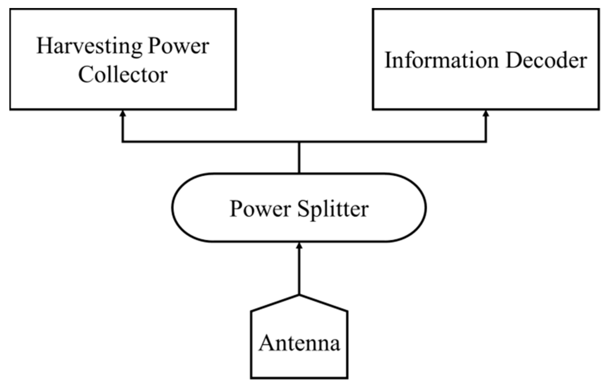
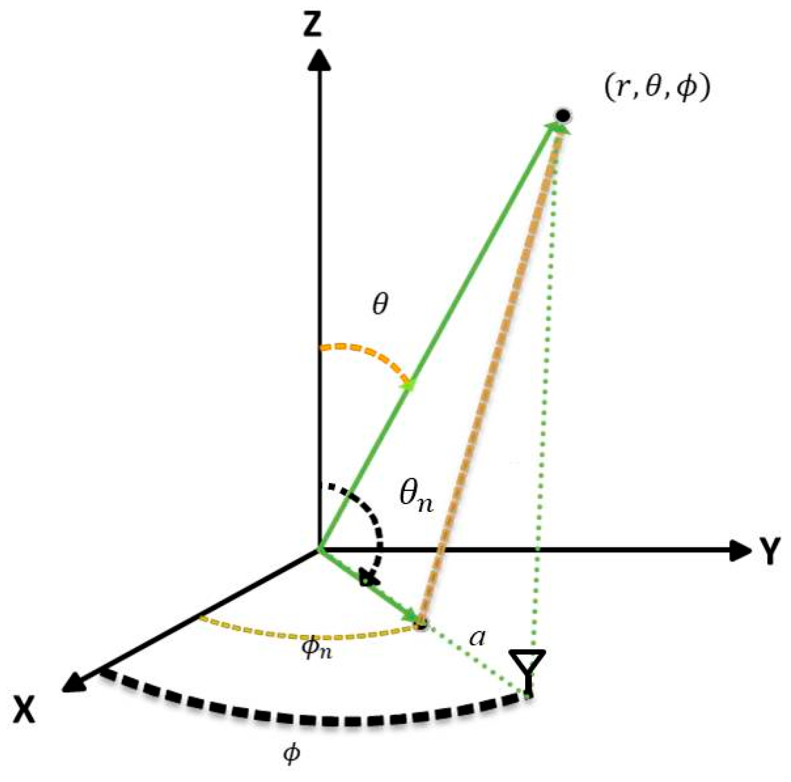
2. System Model
3. Evolution Algorithm
- Step 1
- First, the population parameters are initialized randomly. During the initialization process, the population is initialized as a -dimensional vector, where denotes the number of parameters.
- Step 2
- The -dimensional adjustment parameters are used to calculate the objective function for any antenna array. The objective functions for particles are then evaluated, where denotes the population size. Based on the calculated value from our objective functions, the best particle is updated accordingly.
- Step 3
- In adjusting the control vectors and of the next iteration, the mutation process is composed of arithmetic combination, by adjusting the test vector , which is generated from the parent parameter vector by the following equation:
- Step 4
- In the crossover mechanism, crossover is determined according to the probability of , and the equation is as follows:
- Step 5
- The vector with the smaller objective function is used to update the position of the global best particle.
- Step 6
- Finally, we decide to execute or stop the algorithm according to the iteration number and the convergent condition.
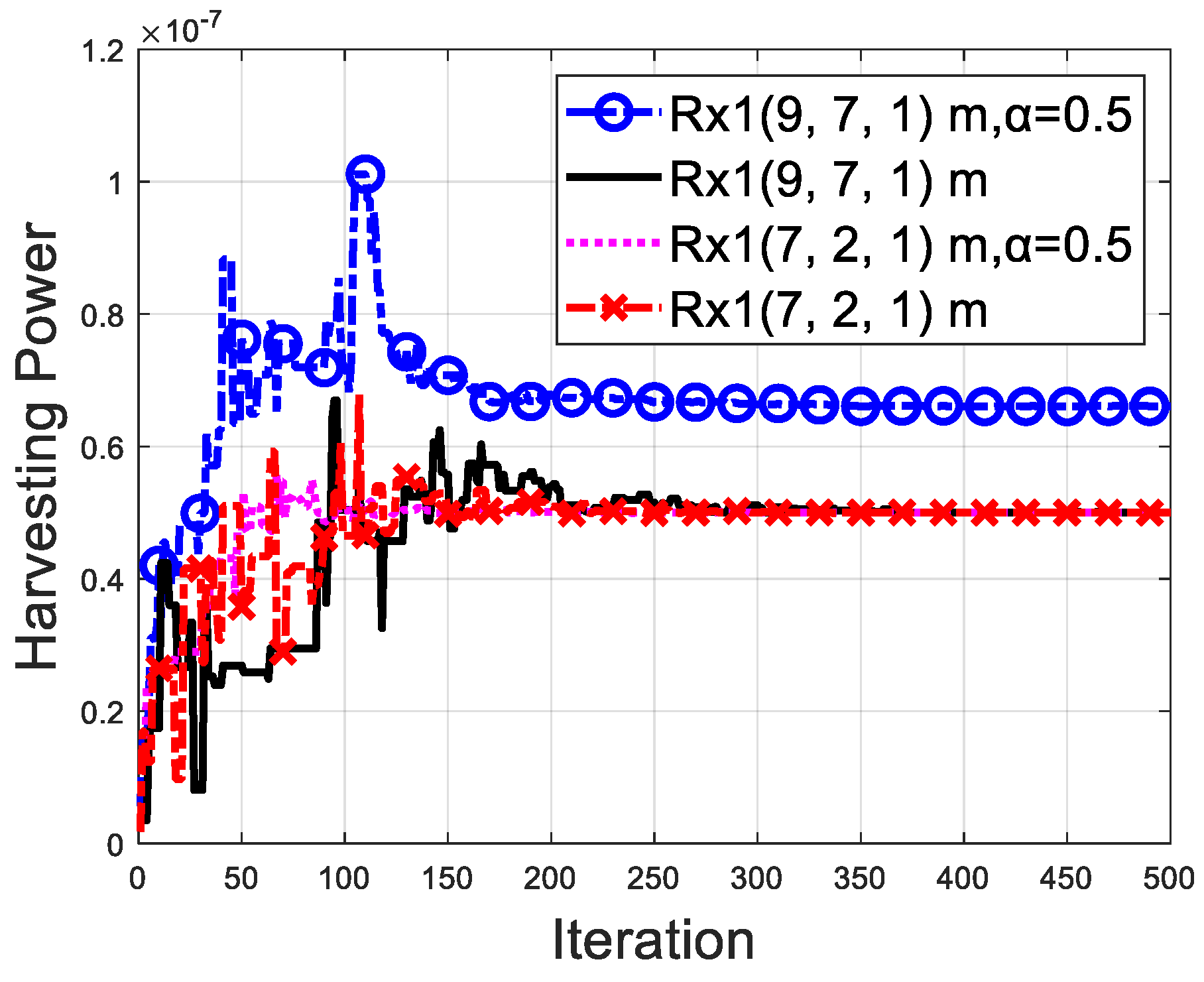
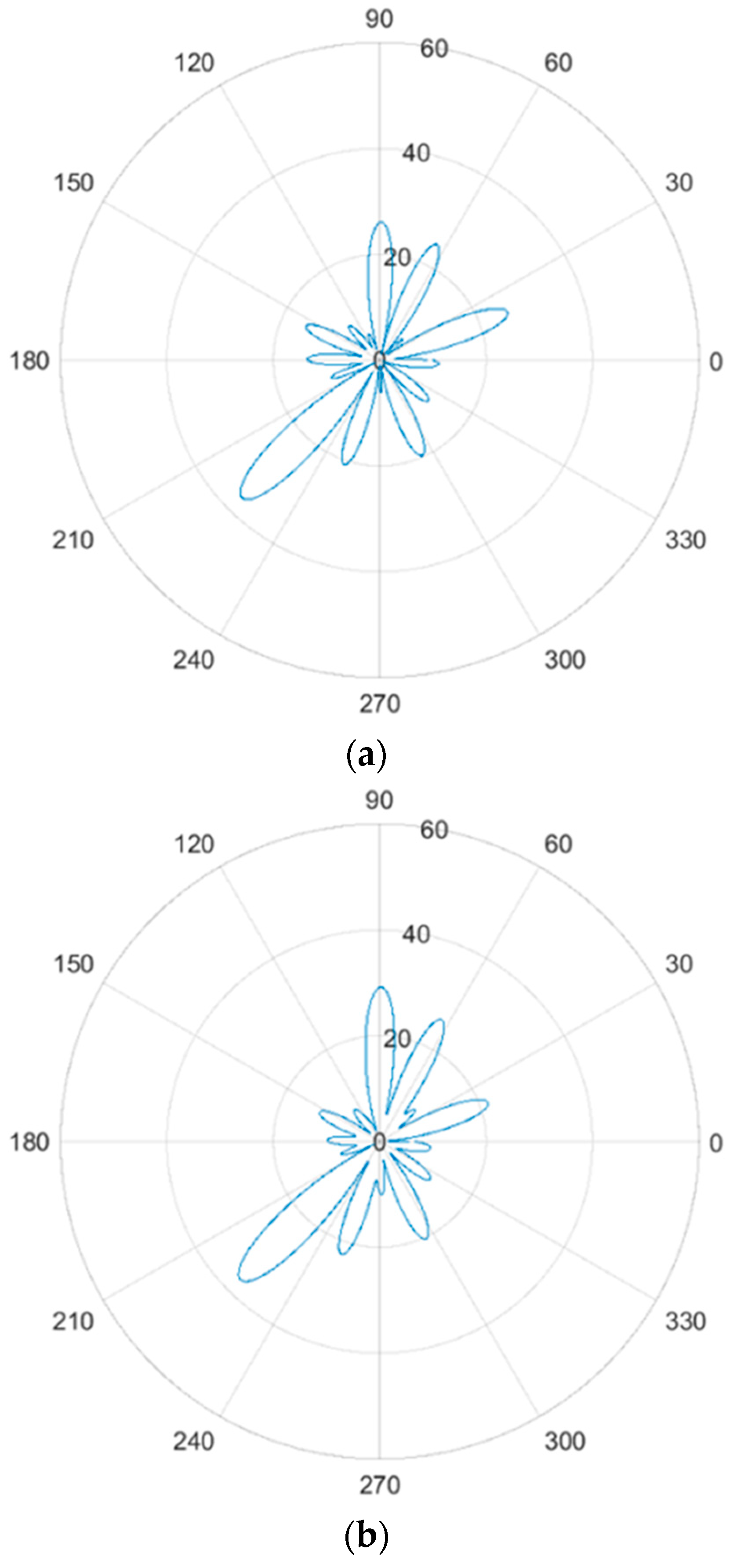
4. Numerical Results
5. Conclusions
Author Contributions
Funding
Institutional Review Board Statement
Informed Consent Statement
Data Availability Statement
Conflicts of Interest
References
- Lee, Y.L.; Qin, D.; Wang, L.-C.; Sim, G.H. 6G Massive Radio Access Networks: Key Applications, Requirements and Challenges. IIEEE Open J. Veh. Technol. 2021, 2, 54–66. [Google Scholar] [CrossRef]
- Tataria, H.; Shafi, M.; Molisch, A.F.; Dohler, M.; Sjöland, H.; Tufvesson, F. 6G Wireless Systems: Vision, Requirements, Challenges, Insights, and Opportunities. Proc. IEEE 2021, 109, 1166–1199. [Google Scholar] [CrossRef]
- De Lima, C.; Belot, D.; Berkvens, R.; Bourdoux, A.; Dardari, D.; Guillaud, M.; Isomursu, M.; Lohan, E.-S.; Miao, Y.; Wymeersch, H.; et al. Convergent Communication, Sensing and Localization in 6G Systems: An Overview of Technologies, Opportunities and Challenges. IEEE Access 2021, 9, 26902–26925. [Google Scholar] [CrossRef]
- Verma, S.; Kaur, S.; Khan, M.A.; Sehdev, P.S. Toward Green Communication in 6G-Enabled Massive Internet of Things. IEEE Internet Things J. 2021, 8, 5408–5415. [Google Scholar] [CrossRef]
- Ansari, R.I.; Chrysostomou, C.; Hassan, S.A.; Guizani, M.; Mumtaz, S.; Rodriguez, J.; Rodrigues, J.J. 5G D2D Networks: Techniques, Challenges, and Future Prospects. IEEE Syst. J. 2018, 12, 3970–3984. [Google Scholar] [CrossRef]
- Shafique, K.; Khawaja, B.A.; Sabir, F.; Qazi, S.; Mustaqim, M. Internet of Things (IoT) for Next-Generation Smart Systems: A Review of Current Challenges, Future Trends and Prospects for Emerging 5G-IoT Scenarios. IEEE Access 2020, 8, 23022–23040. [Google Scholar] [CrossRef]
- Zhou, B.; Liu, A.; Lau, V. Successive Localization and Beamforming in 5G mmWave MIMO Communication Systems. IEEE Trans. Signal Process. 2019, 67, 1620–1635. [Google Scholar] [CrossRef]
- Huang, J.; Xing, C.-C.; Wang, C. Simultaneous Wireless Information and Power Transfer: Technologies, Applications, and Research Challenges. IEEE Commun. Mag. 2017, 55, 26–32. [Google Scholar] [CrossRef]
- Perera, T.D.P.; Jayakody, D.N.K.; Sharma, S.K.; Chatzinotas, S.; Li, J. Simultaneous Wireless Information and Power Transfer (SWIPT): Recent Advances and Future Challenges. IEEE Commun. Surv. Tutor. 2017, 20, 264–302. [Google Scholar] [CrossRef]
- Wang, X.; Gursoy, M.C. Coverage Analysis for Energy-Harvesting UAV-Assisted mmWave Cellular Networks. IEEE J. Sel. Areas Commun. 2019, 37, 2832–2850. [Google Scholar] [CrossRef]
- Ashraf, N.; Sheikh, S.A.; Khan, S.A.; Shayea, I.; Jalal, M. Simultaneous Wireless Information and Power Transfer With Cooperative Relaying for Next-Generation Wireless Networks: A Review. IEEE Access 2021, 9, 71482–71504. [Google Scholar] [CrossRef]
- Park, J.J.; Moon, J.H.; Lee, K.-Y.; Kim, D.I. Transmitter-Oriented Dual-Mode SWIPT With Deep-Learning-Based Adaptive Mode Switching for IoT Sensor Networks. IEEE Internet Things J. 2020, 7, 8979–8992. [Google Scholar] [CrossRef]
- Al-Eryani, Y.; Akrout, M.; Hossain, E. Antenna Clustering for Simultaneous Wireless Information and Power Transfer in a MIMO Full-Duplex System: A Deep Reinforcement Learning-Based Design. IEEE Trans. Commun. 2021, 69, 2331–2345. [Google Scholar] [CrossRef]
- Lu, W.; Si, P.; Huang, G.; Han, H.; Qian, L.; Zhao, N.; Gong, Y. SWIPT Cooperative Spectrum Sharing for 6G-Enabled Cognitive IoT Network. IEEE Internet Things J. 2021, 8, 15070–15080. [Google Scholar] [CrossRef]
- López, O.L.A.; Alves, H.; Souza, R.D.; Montejo-Sánchez, S.; Fernández, E.M.G.; Latva-Aho, M. Massive Wireless Energy Transfer: Enabling Sustainable IoT Toward 6G Era. IEEE Internet Things J. 2021, 8, 8816–8835. [Google Scholar] [CrossRef]
- Wang, J.; Wang, G.; Li, B.; Yang, H.; Hu, Y.; Schmeink, A. Massive MIMO Two-Way Relaying Systems With SWIPT in IoT Networks. IEEE Internet Things J. 2021, 8, 15126–15139. [Google Scholar] [CrossRef]
- Huang, C.; Yang, Z.; Alexandropoulos, G.C.; Xiong, K.; Wei, L.; Yuen, C.; Zhang, Z.; Debbah, M. Multi-Hop RIS-Empowered Terahertz Communications: A DRL-Based Hybrid Beamforming Design. IEEE J. Sel. Areas Commun. 2021, 39, 1663–1677. [Google Scholar] [CrossRef]
- Guo, Y.J.; Ansari, M.; Fonseca, N.J.G. Circuit Type Multiple Beamforming Networks for Antenna Arrays in 5G and 6G Terrestrial and Non-Terrestrial Networks. IEEE J. Microw. 2021, 1, 704–722. [Google Scholar] [CrossRef]
- Cataka, F.O.; Kuzlub, M.; Catakc, E.; Calid, U.; Unale, D. Security Concerns on Machine Learning Solutions for 6G Networks in mmWave Beam Prediction. Phys. Commun. 2022, 52, 101626. [Google Scholar] [CrossRef]
- Jiang, Z.; Wang, Z.; Leach, M.; Lim, E.G.; Zhang, H.; Pei, R.; Huang, Y. Symbol-Splitting-Based Simultaneous Wireless Information and Power Transfer System for WPAN Applications. IEEE Microw. Wirel. Compon. Lett. 2020, 30, 713–716. [Google Scholar] [CrossRef]
- Wagih, M.; Hilton, G.S.; Weddell, A.S.; Beeby, S. Dual-Polarized Wearable Antenna/Rectenna for Full-Duplex and MIMO Simultaneous Wireless Information and Power Transfer (SWIPT). IEEE Open J. Antennas Propag. 2021, 2, 844–857. [Google Scholar] [CrossRef]
- Lu, P.; Huang, K.M.; Song, C.; Ding, Y.; Goussetis, G. Optimal Power Splitting of Wireless Information and Power Transmission using a Novel Dual-Channel Rectenna. IEEE Trans. Antennas Propag. 2022, 70, 1846–1856. [Google Scholar] [CrossRef]
- Jiang, Z.J.; Zhao, S.; Chen, Y.; Cui, T.J. Beamforming Optimization for Time-Modulated Circular-Aperture Grid Array With DE Algorithm. IEEE Antennas Wirel. Propag. Lett. 2018, 17, 2434–2438. [Google Scholar] [CrossRef]
- Zheng, S.; Gao, S.; Yin, Y.; Luo, Q.; Yang, X.; Hu, W.; Ren, X.; Qin, F. A Broadband Dual Circularly Polarized Conical Four-Arm Sinuous Antenna. IEEE Trans. Antennas Propag. 2018, 66, 71–80. [Google Scholar] [CrossRef]
- Hu, Z.; Xie, D.; Jin, M.; Zhou, L.; Li, J. Relay Cooperative Beamforming Algorithm Based on Probabilistic Constraint in SWIPT Secrecy Networks. IEEE Access 2020, 8, 173999–174008. [Google Scholar] [CrossRef]
- Cai, Y.; Cui, F.; Shi, Q.; Wu, Y.; Champagne, B.; Hanzo, L. Secure Hybrid A/D Beamforming for Hardware-Efficient Large-Scale Multiple-Antenna SWIPT Systems. IEEE Trans. Commun. 2020, 68, 6141–6156. [Google Scholar] [CrossRef]
- Wang, B.; Feng, G.; Guo, W.; Sun, Y.; Liu, Y. Achievable Rate of Beamforming Dual-Hop Relay Network With a Jammer and EH Constraint. IEEE Sens. J. 2020, 20, 10123–10129. [Google Scholar] [CrossRef]
- Zhang, J.; Zheng, G.; Krikidis, I.; Zhang, R. Fast Specific Absorption Rate Aware Beamforming for Downlink SWIPT via Deep Learning. IEEE Trans. Veh. Technol. 2020, 69, 16178–16182. [Google Scholar] [CrossRef]
- Chiu, C.C.; Lai, G.D.; Cheng, Y.T. Self-adaptive Dynamic Differential Evolution Applied to BER Reduction with Beamforming Techniques for UItra Wideband MU-MIMO Systems. Electromagn. Res. C 2018, 87, 187–197. [Google Scholar] [CrossRef][Green Version]
- Liu, C.L.; Chiu, C.C.; Liao, S.H.; Chen, Y.S. Impact of Metallic Furniture on UWB Channel Statistical Characteristics. Tamkang J. Sci. Eng. 2009, 12, 271–278. [Google Scholar]
- Chiu, C.C.; Tong, Y.X.; Cheng, Y.T. Comparison of SADDE and PSO for Smart Antennas in Wireless Communication. Int. J. Commun. Syst. 2019, 32, e3941. [Google Scholar] [CrossRef]


| BER | Harvesting Power Ratio | Harvesting Power Ratio Improvement | α | |
|---|---|---|---|---|
| Rx1 | O | 7.15% | 0.5 | |
| Rx2 | ||||
| Rx1 (α) | O | 0.44 | ||
| Rx2 (α) |
| BER | Harvesting Power Ratio | Harvesting Power Ratio Improvement | α | |
|---|---|---|---|---|
| Rx1 | O | 2.6% | 0.5 | |
| Rx2 | ||||
| Rx1 (α) | O | 0.53 | ||
| Rx2 (α) |
| BER | Harvesting Power Ratio | Harvesting Power Ratio Improvement | α | |
|---|---|---|---|---|
| Rx1 | O | 7.87% | 0.5 | |
| Rx2 | ||||
| Rx1 (α) | O | 0.59 | ||
| Rx2 (α) |
| BER | Harvesting Power Ratio | Harvesting Power Ratio Improvement | α | |
|---|---|---|---|---|
| Rx1 | O | 86.7% | 0.5 | |
| Rx2 | ||||
| Rx1 (α) | O | 0.95 | ||
| Rx2 (α) |
| BER | Harvesting Power Ratio | Harvesting Power Ratio Improvement | α | |
|---|---|---|---|---|
| Rx1 | O | 0.13% | 0.5 | |
| Rx2 | ||||
| Rx1 (α) | O | 0.63 | ||
| Rx2 (α) |
| BER | Harvesting Power Ratio | Harvesting Power Ratio Improvement | α | |
|---|---|---|---|---|
| Rx1 | O | 0.52% | 0.5 | |
| Rx2 | ||||
| Rx1 (α) | O | 0.55 | ||
| Rx2 (α) |
Publisher’s Note: MDPI stays neutral with regard to jurisdictional claims in published maps and institutional affiliations. |
© 2022 by the authors. Licensee MDPI, Basel, Switzerland. This article is an open access article distributed under the terms and conditions of the Creative Commons Attribution (CC BY) license (https://creativecommons.org/licenses/by/4.0/).
Share and Cite
Chiu, C.-C.; Chien, W.; Chen, P.-H.; Cheng, Y.-T.; Jiang, H.; Chen, E.-L. Optimization for an Indoor 6G Simultaneous Wireless Information and Power Transfer System. Symmetry 2022, 14, 1268. https://doi.org/10.3390/sym14061268
Chiu C-C, Chien W, Chen P-H, Cheng Y-T, Jiang H, Chen E-L. Optimization for an Indoor 6G Simultaneous Wireless Information and Power Transfer System. Symmetry. 2022; 14(6):1268. https://doi.org/10.3390/sym14061268
Chicago/Turabian StyleChiu, Chien-Ching, Wei Chien, Po-Hsiang Chen, Yu-Ting Cheng, Hao Jiang, and En-Lin Chen. 2022. "Optimization for an Indoor 6G Simultaneous Wireless Information and Power Transfer System" Symmetry 14, no. 6: 1268. https://doi.org/10.3390/sym14061268
APA StyleChiu, C.-C., Chien, W., Chen, P.-H., Cheng, Y.-T., Jiang, H., & Chen, E.-L. (2022). Optimization for an Indoor 6G Simultaneous Wireless Information and Power Transfer System. Symmetry, 14(6), 1268. https://doi.org/10.3390/sym14061268