Abstract
Considering the growing interest in sending probes to the natural satellite Titan, our work aims to investigate and map natural orbits around this moon. For that, we use mathematical models with forces that have symmetry/asymmetry phenomena, depending on the force, applied to orbits around Titan. We evaluated the effects due to the gravitational attraction of the Saturn, together with the perturbative effects coming from the non-sphericity of Titan (the gravitational coefficient ) and the effects of the atmospheric drag present in the natural satellite. Lifetime maps were generated for different initial configurations of the orbit of the probe, which were analyzed in different scenarios of orbital perturbations. The results showed the existence of orbits surviving at least 20 years and conditions with shorter times, but sufficient to carry out possible missions, including the important polar orbits. Furthermore, the investigation of the oscillation rate of the altitude of the probe, called coefficient , proposed in this work, showed orbital conditions that result in more minor oscillations in the altitude of the spacecraft.
1. Introduction
Being one of the largest natural satellites in the solar system, Titan is an exciting body due to its similarities with Earth in many ways, making it one of the targets to be visited by space exploration missions planned for the coming years. After its discovery in the mid-17th century by Christiaan Huygens, the main findings of Titan came only centuries later during astronomical observations led by Gerard Kuiper, published in 1944. These detected methane by using sunlight reflected from Titan that passed through a spectrometer [1], and therefore it was concluded that this moon had an atmosphere. Scientists believed that this atmosphere would be dense and opaque, thanks to the advances in studies and observations made later. With the beginning of the space age, and the overflights on Titan by the Pioneer 11 and Voyager 1 and 2 missions, several predictions were made regarding its thick and extensive atmosphere, as well as its composition, in addition to other physical characteristics such as the temperature of its surface, its radius, and others [2]. However, it was with the Cassini–Huygens mission that more detailed measurements of the surface of the moon could be carried out because, due to its dense atmosphere, the measuring devices of the Voyager 1 and 2 missions were unable to obtain clear images, as was done when the Huygens probe landed on its surface. The data brought by the Huygens probe showed that the atmosphere of Titan is active [3] and that important chemical–organic processes take place in it. It was also seen that climatic cycles based on hydrocarbons occur, which are very similar to the current water cycle on Earth [4], that is, there is the formation of clouds and precipitation in addition to the existence of seas and lakes in the liquid state. Therefore Titan is a body that, in addition to the Earth, currently has an active hydrological cycle [5], thus showing the importance of carrying out missions around this moon. The dragonfly mission that is scheduled for this decade will carry out in situ research of Titan, where samples will be collected to study, in a more profound way, chemical processes in search of life and the methane cycle [6].
In this sense, our work aimed to investigate and map natural orbits around Titan. The study of these effects in the most diverse orbital systems has been investigated over the years. Specifically, the effect of the third body perturbation has been investigated for a long time, and results that started from the determination of the first terms of the perturbative function were obtained in [7,8]. Investigations of the contributions of lunisolar effects [9,10] to the present analytical and computational approaches. Driven by the importance of studying the orbit of the probes and artificial satellites, considering the perturbations due to the action of a third body, ref. [11] presents a study on the orbital evolution of probes around the most important natural satellites, including the Moon and the Galilean satellites of Jupiter. Those investigations sought to locate the initial conditions that would guarantee the orbits that survive for longer times even in the face of disturbances suffered by the action of the third body. The lifetimes of these orbits were estimated for each natural satellite of the Solar System, and the existence of equatorial and frozen orbits was also verified.
Presenting the characteristic of conserving the argument of pericenter and eccentricity, frozen orbits are very interesting scientifically when it comes to lunar orbits since they allow the vehicle to pass always through a given latitude with the same height about to the surface of the natural satellite [12]. Near-polar and low-altitude orbits are also highly relevant in carrying out observation missions, as they allow good coverage of the [13] object. Critical inclination orbits, as well as systems considering the effects due to zonal and sectoral harmonic potentials, have also been investigated over the years [12]. Using a double-average model with expansion in Legendre polynomials to second order, ref. [14] brings a semi-analytical approach together with numerical simulations to study the orbital perturbation produced by a third body in a space probe. This study helps in the scenario of these missions, as it compensates for the absence of formulations that explicitly consider the influence of the eccentricity of the perturber on the perturbing function, in addition to performing a numerical study of three-body systems where the perturbing body is in an elliptical orbit. The present work, based on previous studies [11,15,16], studies the permanence of an artificial satellite in almost circular and three-dimensional orbits around the Moon, considering the action of the Earth. The results allowed us to conclude that the increase in the eccentricity of the orbit of the disturber is responsible for making oscillations in the eccentricity of the orbit of the space vehicle. However, these oscillations reduce the oscillations already presented in the case where the perturbator has a circular orbit.
Considering the study of perturbations of the third body and due to the non-sphericity of the natural satellites, ref. [17] presents part of the study of the gravitational effects due to the third body in a probe that orbits the Moon, considering in this scenario the effects due to the non-spherical distribution of the mass of the natural satellite. The terms due to the second Zonal harmonic () and to the order 2 sectoral flattening coefficient () are considered. Part of the investigations were carried out using the double average method, which is already used in other works. Continuing with those studies, ref. [12] carried out the study of the dynamics of an artificial satellite around the Moon considering its non-sphericity, in addition to the effects of the disturbance coming from a third body, in this case, the Earth. However, in [12], the orbit described by the disturbing body was not circular. Previous works [18,19,20] also presented studies of satellites in mid-altitude regions, considering the effect of the non-sphericity of the central body and the perturbation of a third body, considering high orders in the expansion of the perturbing function, as well as the long-term perturbing effects on high-altitude orbits due to the third body considering in the perturbing function the inclination of the perturbing body.
Results for natural satellites such as Europa were produced by [13], who studied the behavior of a probe orbiting Europa in low orbits, considering in this scenario the gravitational perturbations coming from Jupiter, the third body, and the non-uniformity in the distribution of the mass of the satellite. The gravitational potential of the body was considered with the terms due to the second and third Zonal harmonic ( and ) and to the order 2 sectoral flattening coefficient (). It used Hamiltonian formalism, considering a Hamiltonian with explicit time dependence, as well as the method of averaging over elliptical orbits for the space probe. The results compared the useful life of the studied orbits, making calculations using one and two averages over the motion. Ref. [21] proposed to investigate the stability time of a space probe around a natural satellite in a three-body system, using the Callisto–Jupiter system as a reference but assigning different values for the eccentricity of the disturbing body, considering that the natural satellite is in the center of the reference system and Jupiter the third body. In [22], an analytical and numerical study was carried out considering the lifetime of a probe around Europa in the presence of Jupiter as a third body. The orbits of interest were orbits with low altitude but highly inclined, since this type of orbit takes advantage of the rotation of the celestial body to observe its entire surface more quickly. The simulations took into account the non-coplanarity of Jupiter and Europa. Their results showed lifetime maps for different conditions for the pericenter of probe and initial node and favorable conditions to extend the lifetime of these orbits using propulsive systems. With the same aim of studying moons of Jupiter, ref. [23] carried out studies for Enceladus in search of favorable orbit conditions for carrying out the proposed missions for the natural satellite.
Considering the growing interest in carrying out missions to Titan, our work aims to contribute to future missions through the study and mapping of orbits around this natural satellite.
2. Mathematical Model
Since the objective of this work is to study the stability and lifetime of the natural orbit of a probe around the natural satellite Titan, simulations were carried out assuming the presence of just three bodies: the natural satellite Titan, as the central body; a probe with negligible mass, which orbits Titan in orbit with initial three-dimensional conditions, with orbital elements ; and the planet Saturn, acting as a third disturbing body, describing an orbit, with respect to Titan, that is circular and coplanar. Information about the masses and equatorial radii of Titan and Saturn are presented in Table 1.

Table 1.
Mass values, mass ratios, and the equatorial radius used in the simulations for the planet Saturn and the natural satellite Titan. is the normalized mass of the bodies.
Considering the interest in the study of natural satellites and space probes located in regions extremely close to these satellites, the effects due to symmetry or asymmetry of the mass configurations of these natural satellites and their gravitational fields are significant. Thus, carrying out studies considering the non-uniform distribution of Titan, more precisely, we consider the second Zonal harmonic , which corresponds to the flattening of the natural satellite. Table 2 presents the non-sphericity coefficient and the orbital conditions of Titan. Previous works [13,18] showed the importance of the disruptive effects on the orbit of the probe due to the irregular shape of the natural satellites. The coefficient due to the flattening of Titan is more significant in terms of magnitude.
Table 2.
Orbital period, semi-major axis, and oblateness coefficient of Titan.
As is known from previous work [24,25], a considerably dense atmospheric region is present in Titan. Hence, the effects due to drag are essential for an accurate determination of the dynamics of probes and space vehicles around Titan. Therefore, in our work, we also consider these effects. In general, the equations of motion for the system under study can be described according to [11,26].
being that
and
where, in Equation (1), and are the position vectors of the probe and Saturn, relative to Titan, and , and the mass ratios of the probe, Titan and Saturn, respectively. In Equation (2) to Equation (4), which correspond to the components of the acceleration due to the flattening of Titan, R is the equatorial radius of the natural satellite and is the second harmonic zonal term. In Equation (5) to Equation (7), the components due to the atmospheric drag force are present, where , , and S are the atmospheric density, the drag coefficient, and the probe section area, respectively.
The Saturn and Titan conditions were implemented in a code written in the C language, using the Rebound package [27], which integrated the restricted three-body problem (RTBP). The simulations were performed with the IAS15 algorithm included in the Rebound package. The IAS15 is a 15th-order integrator that can handle conservative and non-conservative forces with adaptive step-size control. It is based on Gauss–Radau quadrature [28] and is accurate down to machine precision [29]. We defined the initial orbital conditions of the probe, . During the temporal evolution of the orbit, the occurrence of escapes from the region of interest of the study were considered, and the simulations were carried out also assuming a collision criterion between the probe and Titan. Considering that this natural satellite has a significant atmosphere, which cannot be neglected in the dynamics, we assumed two criteria for the loss of the probe in our simulations. These collision and escape criteria are described in Section 2.1 and Section 2.2.
All simulations were made using a time interval corresponding to 477 orbital periods of Titan, which corresponds approximately to 20 years. Orbits that did not escape the region of interest and were not classified as lost were considered as orbits surviving the total integration time.
2.1. The Region of Interest Ejection Criteria
In our work, we consider the region of interest for the orbits of the probes as the region of the gravitational domain of Titan, with its gravitational radius of influence being calculated based on [26], by Equation (8):
where is the normalized mass ratio of Titan. In our work, we established as a criterion for escape, or ejection of the probe from the region of interest, an instant when the orbit of the probe has an altitude, in relation to surface of Titan, greater than the radius of the sphere of influence of the natural satellite. Thus, when observed that the altitude of the probe, at time t, was greater than the radius of the sphere of influence of Titan, the probe was considered ejected, being removed from the simulation.
2.2. The Collision Criteria
In addition to the escape criterion, we considered two other forms of probe loss in our work. First, taking into account the presence of an atmospheric region around Titan that can be divided into a denser region, km, and a less dense region, km km [24], we established a first collision criterion considering the loss of the probe upon, in the simulations, the first contact of the probe with the densest atmospheric region of Titan. Therefore, if the orbit of the probe altitude were equal to or less than 600 km, the probe would be removed from the simulation. This criterion was classified as (CollAtm) and can be illustrated by the dotted line in Figure 1. This criterion aims to analyze the lifetime of the orbit of the probe on the surface of Titan, motivated by the interest in using orbits to observe the atmosphere and the surface of the natural satellite in regions not disturbed by the action of more intense atmospheric drag.
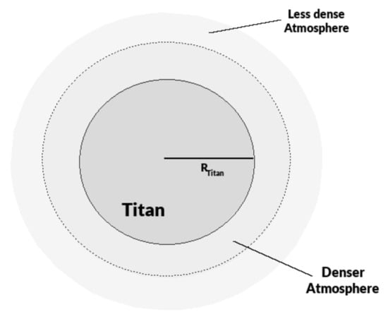
Figure 1.
Scheme of the atmospheric regions of Titan and representation of the probe collision and loss criteria considered in our work. CollAtm—dashed line and CollAlt—solid line.
To later investigate the effects on the lifetimes of the orbits, a physical collision criterion (CollAlt) was considered in the simulations, thus taking into account the probe dynamics in the interval for km. This criterion can be illustrated by the solid line on the surface of Titan in the scheme of Figure 1. Each of the criteria were chosen and simulated individually.
3. Results and Discussion
The results obtained in our investigations were gathered to present, initially, the simulations considering only the third-body perturbations due to Saturn. This is followed by the analysis considering, in addition to Saturn, the contributions due to non-sphericity of the Titan. Subsequently, the orbital regions that contribute to atmospheric drag present on Titan are also analyzed. Finally, we analyze the evolution of the orbital elements of some orbits and present some maneuver proposals.
3.1. The Third-Body Effects of Saturn on the Lifetime of Orbits
For a first analysis of the perturbative effects due to a third body, promoted by Saturn, on the orbit of the probe around Titan, simulations were initially performed considering the collision criterion in the region of the densest atmosphere (CollAlt), described in Section 2.2. In these simulations, the orbits of probe were initially considered circular, and the analysis was later expanded to eccentric initial orbits. For the case of initial circular orbits, investigations were initially carried out for an initial inclination interval between 0° ° and an initial semi-major axis interval between , which corresponds to initial altitudes in the range of km 10,942.5 km. Then, simulations were performed with initial eccentric orbits, in the range of [0.1–0.5], considering the same initial conditions for inclination and semi-major axis, initially assuming that, for the cases of elliptical orbits, the orbital parameters pericenter argument, , ascending node longitude, , and true anomaly, , were zero. The results obtained in the simulations were initially grouped into two groups: Lifetime overview and Lifetime in non-survival regions.
3.1.1. Lifetime Overview
For the first studies, assuming the loss criterion of the probe when entering the densest atmosphere of the Titan (CollAtm), based on Section 2.2, the simulations showed that there is a large region (see in Figure 2) over which the orbits of the probes survived the full integration time so, obtaining lifetimes of at least 20 years. In Figure 2, the limits of these regions are shown by isolines, using different colors for each initially simulated eccentricity in the range of [0.0–0.5]. These regions with orbits lasting at least 20 years are found, in the interval of inclination of 0° °, in the lower regions of the isolines and the interval of inclination of 90° °, in the superior regions of the isolines, corresponding to each value of initial eccentricity of the orbits. In the case of circular initial orbits (line in black) conditions extend throughout the initial semi-major axis range between , which corresponds to initial altitudes in the range of km km. There is also a symmetry with the axis at 90° for the behavior of the surviving orbital regions. This behavior was observed for all eccentricities simulated. It is worth mentioning that, since in the simulations it is assumed that all orbits are implemented with zero true anomaly, the regions where the isolines start, for each initial simulated eccentricity, correspond to the initial orbits whose initial altitudes have a value greater than 600 km, because the regions before the beginning of the isolines on the lower inclinations, 0°, as shown on the maps, produce initials radius at the altitude of the densest atmosphere of Titan determined for this work.
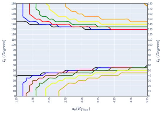
Figure 2.
Mapping, as a function of initial inclination and semi-major axis, of regions with orbits around Titan having lifetimes greater than or equal to 20 years and less than 20 years, considering different values for the initial eccentricity of the orbit of the probe: (black) for circular orbits, (blue) for , (red) for , (green) for , (yellow) for , and (orange) to . Simulations performed considering the loss of the probe at an altitude of km (CollAtm).
Based on the simulation criteria presented in Section 2.1 and Section 2.2, the final conditions of the orbits were classified into three groups: orbits that collided, escaped the region of interest, or survived the total integration time. Overall, the results showed that orbits that did not survive the total integration time of 20 years were considered lost by collision. Therefore, no escapes from the region of interest were recorded. This behavior shows that these orbits entered the densest atmosphere of the Titan, km, at some point during their temporal evolution. This behavior was observed for both initial circular and eccentric orbits ().
3.1.2. Lifetime in Non-Survival Regions
Based on the behaviors observed in the maps of Figure 2, it was seen that for the entire initial eccentricity interval of , the region for the initial inclination between 50° and 130° is a typical interval where the orbits of probes did not survive the full integration time, being considered lost for entering the atmosphere of Titan at some point in their temporal evolution. As it is interesting to investigate this region to see how the lifetimes of the orbits of probes behaved, we performed simulations in the region of 50° to 130° for the initial inclination of the interval and semi-major axis, , where corresponds to the largest equatorial radius of Titan, and eccentricity . The initial inclinations of 65° to 120° are shown in Figure 3, where lifetime maps were built. In these maps, initial conditions whose semi-major axis already produces orbits with an initial orbital radius less than km were omitted. The results obtained for the intervals of 50° to 65° and 120° to 130°, however, were only described in the text.
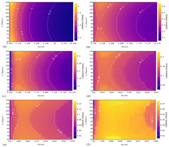
Figure 3.
Lifetime maps of the orbits of the probe around Titan, as a function of initial inclination and altitude , for the intervals 65° ° and different initial orbital eccentricities: (a) ; (b) ; (c) ; (d) ; (e) ; and (f) . Simulations performed considering the loss of the probe at an altitude of km (CollAtm) and only disturbances due to Saturn.
The results show that, for the orbits around Titan that did not survive the total simulation time, the lifetimes show a dependence on the choice of the inclination value, the semi-major axis (orbital radius), and the initial eccentricity. There is a greater dependence on the eccentricity and the initial semi-major axis. The maps show that when the orbits are implemented with larger eccentricities, the lifetimes are smaller, and, for fixed initial eccentricities, the initial semi-major axis increases. So the increase in the initial orbital radius also contributes to shorter orbit lifetimes. These behaviors can be explained by the fact that the perturbation of the third body, Saturn, affects the eccentricity of these orbits, making them more eccentric in a shorter time, thus favoring the loss by collision in the atmosphere, or the escape of the region of interest of the probe. The influence of the choice of the initial semi-major axis can be better seen in the maps fixing the initial eccentricity because orbits with a higher initial semi-major axis have a larger initial orbital radius, thus exposing the probe to a more significant influence of Saturn, which tends to promote greater perturbations, leading to shorter lifetimes for the orbits. The choice of the initial inclination is also an important factor, although with less influence compared to the choice of and , because in the range of ° ° the orbits decrease lifetime as the inclination increases from ° to initial polar orbits and as they decrease from ° to °, reinforcing the observations about the symmetry with an axis at °. These results will be further detailed in Section 3.5.
In terms of the lifetimes of the probe orbits, in the range, ° °, Figure 2, shows that the initial circular orbits had more records of orbits with the longest lifetimes because orbits with durations in the range from 87 days to years were found. For , the lifetimes showed a sharp drop concerning the circular orbits, recording lifetimes in the range of 49 to 177 days. Orbits with durations between 17 and 104 days, for , and between 30 and 74 days, for , was also found. For more eccentric initial orbits, such as , most orbits recorded time between 18 and 42 days in duration. When the simulations considered an initial eccentricity of , the lifetimes were between and 30 days in duration.
In the range of ° ° and ° °, it is also observed that the initial circular orbits had more orbits with the longest lifetimes, because orbits with a duration in the range from 183 days to years were found. For , the lifetimes showed lifetimes in the range of 76 days to 1 years. Highlighting the orbit with and °, which has a lifetime of approximately 7 years. For and , orbits with lifetimes between 2 days to years and 35 days to 1 year were registered, respectively. The lifetimes of the orbits for e have values between 18 to 55 days and 2 to 33 days, respectively.
3.2. The Effect Due to the Non-Sphericity of Titan
Considering the interest in studying orbital regions extremely close to natural satellites, the effects of the mass configurations of these natural satellites are essential. Some bibliographic references, such as [21,30,31], indicate that the flattening of the central body can offset the effects of a disturbing third body, helping to find more stable orbits. In this sense, in our work, we consider the effects coming from the non-sphericity of Titan in our simulations. More specifically, the simulations were performed considering the zonal harmonic coefficient of Titan (see Table 2). These simulations were performed, initially, considering the same conditions presented in Section 3.1.2, keeping the criterion of collision or loss of the probe by contact with the denser atmosphere of Titan. The results considering the zonal harmonic allowed us to observe that, in general, the behaviors of the lifetime maps do not change significantly in relation to the maps considering only the perturbations originated from Saturn. Based on the results obtained in the simulations considering only perturbations from Saturn and considering the perturbative actions from Saturn and the contribution due to of Titan, it was calculated the variations in these orbit lifetimes, which showed that most orbits maintained, in terms of months, the same chosen lifetimes without the action of then non-sphericity of Titan.
In terms of the initial eccentricity of the orbits, it appears that, in addition to the more significant number of long-lived orbits found in initial circular orbits, the effects due to the flattening of the natural satellite also acted more significantly in these orbits, registering slightly more significant gains or losses in the duration of the lifetimes of the orbits. However, for probes placed in an eccentric initial orbital, we observed some conditions with significant gains or losses in life were also encountered. That when the initial eccentricity increased, the variations in lifetime decreased. In terms of lifetime values, orbits implemented with an initial eccentricity did not gain more than 1 day in duration, and the duration of the orbit was in the range between 1 and 6 days. In the dynamics considering , most orbits did not show gains or losses greater than 5 days. However, an orbital condition was found for the inclination of 50° and initial semi-major axis km with an initial altitude of km, where a gain of approximately years in the life was observed. Due to flattening of Titan, the orbit had a total duration of years with this gain. For orbits implemented with , orbit times gains of more than 7 days were not found, as well as orbits with lifetime losses were also not larger than 5 days. Although in the simulations considering , most orbits have registered gains or losses of less than 6 days, two orbits were found, with ° for km and ° for km, with gains of 7 and 19 years. For , most of the gains or losses were not of more than 6 days. In the case of the simulations carried out considering the initial circular orbits, the results showed that most of the orbits do not present changes in lifetimes larger than 1 day. However, for the region of lower initial altitudes, close to 600 km, the largest gains, and losses in orbit lifetimes were found. Due to the flattening of Titan, a large concentration of these changes is seen in the initial inclinations close to 50, 60, 90, 120, and 130 degrees. The orbits generated by these initial conditions had losses of up to 36 days. The observed increments were found, in general, in three large intervals: orbits with gains of up to 36 days, orbits with gains of up to 2 months, and orbits with gains of 3.5 months. Orbits were also found that, due to gravitational perturbations of Titan, became orbits surviving the total time of integration, as they showed gains of 15 and 19 years. These orbits have km for ° and km for °, respectively. In general, the first results considering the zonal harmonic showed that, depending on the initial geometry of the orbit implementation possible, there are local conditions where the gains or even losses in the lifetime of the orbits can be considered for possible missions around Titan. Previous works such as [17,32] also show results showing results with similar behavior for probe studies around other natural satellites considering their effects due to . Furthermore, it was observed that the increments or losses in lifetimes in these simulations determined the duration of the orbits at altitudes above the denser atmosphere of Titan, as defined previously.
3.3. Contribution of the Altitude Region of Less Than 600 km in Lifetimes of the Probe
So far, the simulations carried out in Section 3.1 and Section 3.2 had a criterion of loss of the probe as the first contact with the denser atmosphere of Titan (CollAtm). Aiming to investigate the contribution of this region with less than km in altitude in the lifetimes of the orbits, new simulations were performed, replacing the probe loss criterion at an altitude of km (ColLAtm) with a physical collision when the altitude of probe is zero (CollAlt), characterizing a contact between the probe and the surface of Titan. Although the simulations took into account the region below km, the effects of atmospheric drag in the region were not considered, initially considering only the perturbations of the third body from Saturn and the effects due to the non-sphericity of Titan. Figure 4 shows the maps obtained in these new simulations.
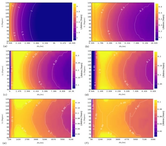
Figure 4.
Lifetime maps of the orbits of a probe around Titan, as a function of initial inclinations and altitude , for the intervals 65° ° and different initial orbital eccentricities: (a) ; (b) ; (c) ; (d) ; (e) ; and (f) . Simulations performed considering the loss of the probe on the surface of Titan (CollAlt) and perturbations due to Saturn and the zonal harmonic of Titan.
In the maps shown in Figure 4, the regions to the right of the vertical dotted line present the results obtained with the same initial conditions as the maps shown in Figure 3. These initial conditions produced orbits with an initial radius greater than 600 km, thus being initiated outside the assumed region for the presence of atmospheric drag. Considering this initial semi-major axis range and thus the initial altitude of the orbits of probe, the results, as expected, showed an increase in the lifetime of the orbits. This increase is due precisely to considering the dynamics of the orbit of the probe in the region below the value of km. These lifetime gains were recorded in both initial circular and eccentric orbits. In the cases of initial eccentric orbits, the gains in lifetimes are in the range of 3 days to 4 months. It was also observed that the most significant gains in lifetimes were found in regions of lower altitude for all simulated cases. Due to the slightest third-body perturbation due to Saturn, the initial circular orbits showed the most significant gains in orbit lifetimes, reaching increments of up to 11 months of orbit. It is noteworthy that, although the collision criterion has been changed, all simulated orbits, which did not survive the total integration time, were classified as collided. Thus, there is no record of escapes from the region of study.
When the collision criterion was assumed to be a physical collision (CollAlt), it was possible to obtain some initial orbital conditions between surface of Titan and an altitude of 600 km, the region at the left of the red vertical dotted line. This group of orbits has the most extended lifetimes found for all simulated initial eccentricity conditions among the simulated initial conditions.
The increase in the lifetime of the orbits simulated by the new collision criterion (CollAlt) and the high times obtained in the simulations that started below the altitude of the atmosphere are factors to be observed because they show that a probe can have a specific time of its dynamics in an altitude region lower than km. So, while many orbits have a longer orbital flight time above surface of Titan, it is also possible to observe at lower altitudes, at least for a few moments, without imminent loss of the probe. How is the presence of an atmosphere on Titan known? We propose a model for the study of orbits around Titan, Section 3.4, considering the presence of atmospheric drag over the region below km altitude, added to third-body perturbations from Saturn and the flattening of Titan.
3.4. The Effect Due to Atmospheric Drag
The simulations considering Saturn perturbations and Titan flattening, assuming the probe’s physical collision with surface of Titan, Section 3.3, show that there are orbital conditions generated with gains of up to months. These results show that, during their orbital evolutions, the probes can stay at an altitude of less than km. As we assume that the atmospheric drag in the region below km is more intense, simulations were carried out considering an atmospheric drag model added to perturbations of Saturn and the non-sphericity of Titan, aiming to observe how the action of atmospheric drag in these regions can interfere in the lifetime of the orbits. The model for the atmospheric density used in our simulations was based on the studies of [24,25,33]. In [33], three models for the decay of atmospheric density of Titan as a function of the altitude of the probe are proposed, with precision for minimum, maximum, and average curves. Although [33] and other works present a model based on the Cassini–Huygens mission, more recent studies, such as [24], present empirical models that are very similar to others, albeit with certain improvements, but all within the curves established by [33]. Work carried out for this purpose shows that, although these models show the behavior of the atmospheric density until close to km of altitude, lower altitude regions, with km, are important, precisely for the study and modeling of orbiter missions that can encounter the atmosphere many times or continuously [24], as shown in the results of Section 3.3. Figure 5 shows the behavior of the atmospheric density model assumed in our work.
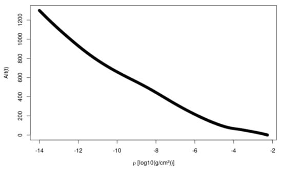
Figure 5.
Atmospheric density model for Titan used in simulations based, on [24,25,33].
Analyzing the atmospheric density model presented in Figure 5, simulations were carried out considering the effect of the third body given by Saturn, non-sphericity of the Titan, and atmospheric drag in the region below 600 km of altitude. As well as the drag region, the criterion of physical collision (CollAlt) was considered. It was verified as possible escapes from the orbit of the probe in the region of interest or the loss by collision with the surface of Titan. The probe had a mass of kg, a radius of m, and a drag coefficient .
In comparison to the maps obtained considering the perturbations of Saturn, the non-sphericity of Titan, and the criterion of the collision on the surface of Titan without atmospheric drag (see Figure 4), the results taking into account the effects of the atmospheric drag show that the times found in these simulations, for the eccentricities in the range from to , showed significant differences. Therefore, the orbits registered contributions from the region inferior to km smaller than those obtained without the drag effect, where gains in the order of months were registered. This shows that, in these cases, the drag acted such that it favored the loss of the probe, thus reducing the time for carrying out possible missions. However, for orbits implemented with initial eccentricity from to , the results started to split into two groups: some orbits are still lost faster due to drag, but, in the more eccentric cases, the drag effects in combination with the non-sphericity of Titan and third body perturbations from Saturn, generate orbits with longer durations compared with the maps obtained considering the perturbations of Saturn, non-sphericity of Titan, and the collision criterion on the surface of Titan without atmospheric drag (see Figure 4). These results show the importance of considering the effects of drag at lower altitudes of Titan, as these effects change the scenario of the lifetimes, being an important factor to consider for possible missions.
It is interesting to note that the results obtained in these simulations were, for the range from to , in most cases, considered close to the results obtained considering the probe loss model at an altitude of 600 km (CollAtm) in Section 3.1.2 and Section 3.2. Figure 6 shows the cumulative distribution of duration time of orbits over the drag region in terms of days for circular and eccentric orbits. In terms of the possibility of missions around Titan, the cumulative distribution of duration time of orbits over the drag region is important, because previous work [34] shows possible designs for future missions that aim to carry out studies with space vehicles in the region atmospheric of Titan. Therefore, for these missions, the cumulative distributions presented aim to guide the duration of the probe’s orbit, over the drag region, before its loss by collision with the surface of Titan. Contributing to estimating the time and planning of measurement missions and sending data in these regions. Thus, it is concluded that the approach considering the CollAtm collision criterion is, to a certain extent, a precise approach to be used in the study of natural orbits around Titan, as it is a good criterion for a first study around Titan. However, as already mentioned, the drag in the region below km in more eccentric orbits, to and with higher altitudes, can promote lifetime increases in some cases, it is interesting to use a CollAlt collision criterion. Thus, depending on the type of mission and its interests, it is possible to use one of the criteria we used and obtain accurate results for the lifetimes of the orbits.
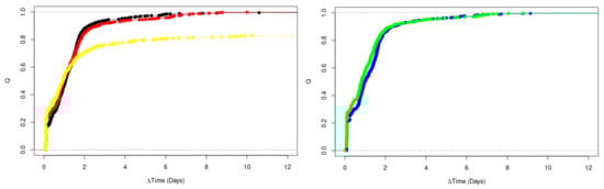
Figure 6.
Cumulative distribution, Q, of the duration of the probes’ orbits in the atmospheric drag domain region below km altitude, before they collided with the surface of Titan. Results for differents values of the eccentricity: (black) for circular orbits, (blue) for , (red) for , (green) for , (yellow) for .
Another essential point shown in Figure 6 is that the results show the possibility of missions in the final time of the orbits to investigate the atmosphere of Titan, since the decay times of the orbits can reach 12 days, a time that is good enough to complete more observations.
The Effect of Atmospheric Drag in the Region of Lower Atmospheric Density
Based on the results obtained in the simulations, considering the atmospheric drag in the lower region at an altitude of km, we investigated how the atmospheric drag present in the less dense region of the atmosphere could interfere with the lifetime of the orbits. For this, we performed simulations considering the effects of the third body due to Saturn, the non-sphericity of Titan, and the atmospheric drag in the altitude region between km and km, based on Figure 5. In these simulations, we kept the initial condition grids, the escape criterion based on radius of influence of Titan, and the probe loss criterion when entering the densest region of the atmosphere, CollAtm. The results obtained are shown in Figure 7.
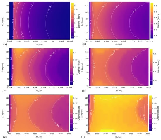
Figure 7.
Lifetime maps of the orbits of probe around Titan, as a function of inclinations and altitude initial, to the intervals 65° ° and different initial orbital eccentricities: (a) ; (b) ; (c) ; (d) ; (e) ; and (f) . Simulations performed considering the loss of the probe at an altitude of km (CollAtm) and the perturby due to Saturn, the harmonic zonal of the Titan and atmospheric drag between the altitudes of km to km.
Based on Figure 3, the results in Figure 7 show that the general behavior of the graphs is maintained, even considering the action of atmospheric drag in the region between km and km of initial altitude. There is a greater dependence on the choice of eccentricity and initial altitude of the probe and thus on the initial semi-major axis. In orbits with larger eccentricities, the lifetimes are shorter. For fixed initial eccentricities, the value of the initial semi-major axis of the orbits and, therefore, the increase in the initial orbital radius also contributes to shorter lifetimes.
One change observed was that in the case of simulations considering the Saturn effects, the zonal coefficient and an atmospheric drag between km and km, for all simulated initial eccentricities, orbits with much lower initial altitudes than km show a significant loss in lifetime, evidencing the effects of the atmospheric drag on Titan.
In terms of the orbital lifetimes of the probe, it is observed that initial circular orbits still have the most number of orbits with longer lifetimes, as orbits lasting up to 3 years were found, in the range of 65° ° and orbits with times between 3 and 17 years in the intervals of 50° ° and 120° °. For the lifetimes showed a sharp drop compared to circular orbits, with lifetimes of up to 222 days. In terms of the simulations without drag, gains of up to 10 days and losses of approximately 292 days were found.
For , some orbits lasted up to 129 days. Orbits lasting between 17 and 80 days were also found, for . The orbits with the highest losses were found at with °, with °, and with ° that recorded losses of 13, 11, and 2 years, respectively. Only one orbit, with °, with a gain of 2 years was found.
In the case of , the orbits, in general, had durations from 1 to 55 days. Having orbits with high lifetimes such as the cases with ° and with °, the orbits with lifetimes of 13 and 2 years, respectively. In the case of , the orbits recorded lifetimes in the range of 2 to 32 days. Compared to the simulations without the drag action, they had gains of up to 8 days and losses of only 3 days.
After the study and mapping of orbits as a function of initial inclination, eccentricity, and semi-major axis, the simulations began to investigate the effects, on lifetimes, of the choice of the initial pericenter argument, , and node longitude, . To this end, simulations were performed around Titan, considering polar orbits and assuming a fixed value for the initial semi-major axis. These simulations were performed for initial eccentricities of , and . These conditions were maintained for the entire pericenter argument grid and initial node longitude in the range of [0–360], always keeping for the true anomaly. The maps obtained are shown in Figure 8.
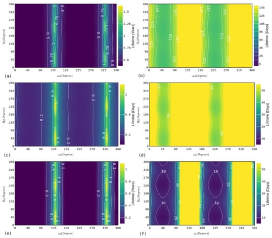
Figure 8.
Lifetime maps of the orbits of a probe around Titan, as a function of the initial pericenter argument and ascending node longitude , for initial polar orbits with a semi-major axis and initial eccentricities (a,b) , (c,d) , and (e,f): . Simulations performed considering the loss of the probe at an altitude of km (CollAtm) and the perturbation from Saturn, the harmonic zonal of Titan and atmospheric drag between the altitudes of km to km.
Figure 8a,c,e present the maps of lifetimes as a function of the pericenter argument and the ascending node longitude in terms of years. Figure 8b,d,f show the maps of the same regions in (a), (c), and (e), respectively, but highlighting other regions, showing the results in terms of days. In general, the maps show that there are regions for the initial (pericenter argument) and (node longitude) arranged on the maps in several vertical bands, which give orbits with longer lifetimes. In terms of the initial pericenter argument, these regions are limited to the range of [90–180] and [270–340] for the entire range of [0–360].
The lifetimes found for the case of , ° and , Figure 8a,b, show orbits with lifetimes between 105 and 499 days. The orbit lifetime for ° and ° is 146 days. The durations obtained, varying the node longitude and the pericenter argument, show gains of up to 352 days and a loss of up to 41 days. In the simulations considering , ° and , Figure 8c,d it is found orbits with lifetimes between 44 and 444 days. The orbit lifetime for ° and ° is 826 days. The durations obtained, varying the value of the node longitude and the pericenter argument, show gains of up to 361 days and a loss of up to 37 days.
For the case of , ° and , Figure 8e,f, it is found orbits with lifetimes between 7 and 411 days. The orbit lifetime for ° and ° is 23 days. The durations obtained, varying the value of the node longitude and the pericenter argument, show gains of up to 387 days and a loss of up to 15 days. The longest times are found in isolated regions within the vertical bands in all maps obtained. These results show that, for the simulated region, there is a greater influence on the initial argument of the pericenter of the orbit of the probe than on the longitude of the ascending node. Thus, for orbits closer to the natural satellite, there is an imbalance in relation to the choice of and because even though the value of the longitude of the node does not present large differences in the lifetimes, a good choice for the pericenter argument can give considerable gains, thus allowing longer mission durations.
3.5. The Evolution of Orbital Elements and the Altitude Range of the Orbits
Considering the lifetimes observed in regions that did not survive the total integration time, a more detailed investigation was carried out to observe the temporal evolution of the orbits. The dynamics showed that, for the cases simulated considering only the perturbation due to Saturn, the eccentricity of the orbits increases as the orbit time increases. Thus, the initially circular orbits tend to become eccentric as Saturn’s third-body effects act on the dynamics of the probe. This behavior can be seen in Figure 9, which presents the evolution of some orbits considering the probe losses due to collision with surface of Titan (CollAlt). The same behavior was seen in the cases considering the probe loss in the atmosphere of the Titan (CollAtm). The results also show that, although the eccentricity of the orbits increases with time, there are small oscillations during this period. These oscillations become more evident when the orbits are located at higher altitudes because, in these configurations, the third-body effects produced by Saturn are more intense due to the proximity to the planet. This behavior for the eccentricity of the orbit of the probe is more expressive for the more eccentric initial orbits. Thus, initial circular orbits generate orbits with longer lifetimes is justified. These observations reinforce the utility of circular orbits in the case of missions with orbiters. In terms of the initial inclination, it was seen that within the inclination range between 50° and 90°, the eccentricity of the orbit grows faster. It is the Kozai–Lidov effect that dominates this range of orbits. Previous works have already mentioned this effect on the orbit of probes [11,21,32], and on irregular natural satellites [35]. For the range of 90°°, the opposite behavior is observed because, as the probe is implemented in more inclined orbits, the eccentricity grows at a lower rate, taking a long flight, so that the orbit becomes eccentric.
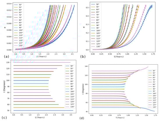
Figure 9.
Evolution of the inclination and eccentricity of the initial circular orbits not surviving the total integration time. Cases of semi-major axis initial equal to (a–c) and (b–d).
The evolution of these orbits also showed that, although the inclination has small oscillations (see Figure 9), the orbits tend to maintain their inclination close to the initial value. This behavior is better observed as the initial inclination of the probes approaches 90°. This is an interesting result because, although the orbits tend to decrease lifetimes as the initial inclination approaches 90°, they have durations large enough to make missions, as seen in Figure 3, in addition to keeping their inclination always close to the initial value. Thus, it is possible to carry out missions in polar and quasi-polar orbits, orbital conditions that stand out for carrying out missions with orbiters. Interestingly, this behavior was observed only in the orbits that did not survive the total integration time. The initial conditions surviving 20 years maintained the oscillations in eccentricity and inclination, as shown in figure Figure 10. However, their period of oscillation was considerably smaller compared to the cases that collided.
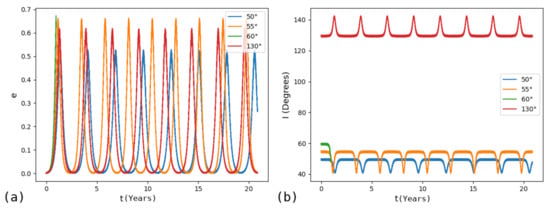
Figure 10.
Evolution of the eccentricity (a) and inclination (b) for initial circular orbits surviving the total integration time.
To investigate the effects due to Saturn perturbations, the Titan flattening and the atmospheric drag on the altitude of the orbits, we define the coefficient , which is determined by Equation (9). It determines the intensity of the altitude oscillation amplitude per lifetime of the orbit, based on the average altitude value.
where is the altitude of probe as a function of time, is the average orbital altitude of the probe over the entire orbit time, and is the duration of the time interval of the orbit of the probe. Figure 11 presents the value of the coefficient for the dynamics considering only the third-body perturbations due to Saturn, (Figure 3). The results show that the orbits tend to have their altitudes less disturbed when implemented at lower altitudes. This can be seen by the darker regions on the graphs representing the smallest values of the coefficient. This behavior was observed in all cases of the initial eccentricity simulated and both probe loss regimes. This fact was also observed in the simulations considering only the perturbative effects of Saturn and in those where the non-sphericity of Titan was added. The results also show that as the orbits are implemented with larger initial eccentricities, the coefficients grow, reinforcing that the more eccentric the orbits, the larger the variations in the altitude of the probe over the lifetime of the orbits. Considering that the initial circular orbits were the ones that registered the largest number of orbits with the longest lifetimes, Figure 11a presents the coefficient for the initial circular orbits. Given the results observed, it is conclusive that the best region for circular orbits that keep the oscillations in altitude lower are those implemented with values below 3500 km. The dynamics of the orbits also allowed us to observe that even with different altitude oscillation rates, it is a behavior of the amplitude of the orbits to keep their altitudes very close to their initial values until moments close to the half-life of their orbit.
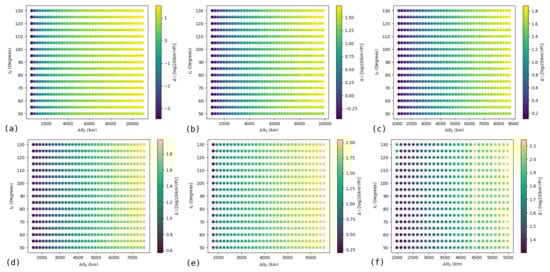
Figure 11.
Maps of the coefficient as a function of initial inclination () and altitude () for different initial orbital eccentricities: (a) ; (b) ; (c) ; (d) ; (e) ; and (f) . Simulations performed considering the loss of the probe on the surface of Titan (CollAlt) and only the perturbation from Saturn.
Figure 12 presents the variation of the coefficient in relation to the simulations considering the coefficient of Titan and the simulations including only the perturbations of the third body of Saturn. In these maps, it can be seen that the altitudes, in general of the probe, fall into two groups: regions where the action of dampens the third-body effects and regions where effects due to accumulate with the third body to increase the oscillations in the altitude of the probes’ orbits. These regions can be located on the maps by the negative regions for an orbit in which the Titan’s flattening effect decreases the average oscillations in the altitude of the probe and the positive regions on the maps, which correspond to more disturbed orbits, thus generating larger oscillations in the altitude of the orbits. In general, regions with an increase in amplitude of the oscilations are dominant, for all simulated initial eccentricities. Especially in orbits with lower initial altitudes, where the non-sphericity action of Titan is more dominant. However, it is very important to mention that the orbits that have compensation between the third-body perturbation and the are very important for real missions.
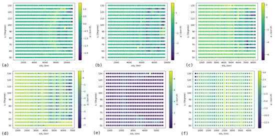
Figure 12.
Maps of the variation of coefficient as a function of initial inclination () and altitude () from different initial orbital eccentricities: (a) ; (b) ; (c) ; (d) ; (e) ; and (f) . Simulations performed considering the loss of the probe on the surface of Titan (CollAlt), the perturbation from Saturn and from the harmonic zonal of Titan. ().
In the case of the maps of the coefficient for the simulations considering the perturbations of Saturn, the non-sphericity of Titan and the atmospheric drag are shown in Figure 13. The same behaviors can also be observed. There are many orbits with greater amplitudes of oscillation due to the action of atmospheric drag. This is an expected result since atmospheric drag contributes to the variations of the semi-major axis and, consequently, the altitude variation of the probe. Circular orbits were the least affected. These results are important and interesting, as they show the possibility of implementing low-inclination circular natural orbits or even polar orbits around Titan.
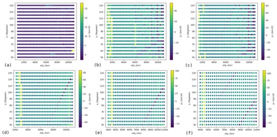
Figure 13.
Maps of the variation of coefficient as a function of initial inclination () and altitude () for different initial orbital eccentricities: (a) ; (b) ; (c) ; (d) ; (e) ; and (f) . Simulations performed considering the loss of the probe on the surface of Titan (CollAlt) and the perturbation due to Saturn, the harmonic zonal of Titan and atmospheric drag between the altitudes of km to km. ().
3.6. Orbital Maneuvers
The results for the lifetimes of the orbits, initially circular, around Titan, considering the perturbations of Saturn, the non-sphericity of Titan, and the atmospheric drag (Figure 7a and Figure 8a), showed the existence of natural polar orbits within the range of [88–786] days. Previous works reinforce the importance of studying and mapping celestial bodies in orbits of this type. In this sense, we propose to carry out orbital maneuvers to relocate these probes at some point before they enter the densest atmospheric region of Titan, in the initial position of their circular orbit. It means that we seek to extend the lifetime of these orbits, thus favoring the accomplishment of missions in these configurations.
We propose to perform the necessary calculations to perform the maneuver at several moments of the orbit’s lifetime, trying to find the best moment to perform them. In other words, we calculate the impulses, and thus the fuel cost, for carrying out the maneuver at different times to obtain the moment with the lowest fuel consumption. The calculations were performed based on Equations (10)–(12).
To transfer the probe from its current elliptical orbit to its initial circular orbit, we try to obtain the value of the magnitude of the velocity required to move the spacecraft its current orbit from to the transfer orbit, , and then the magnitude of the velocity variation required to place it in the circular target orbit, . is the radius apocenter of the elliptical orbit before the maneuver, and is the radius of the circular orbit after the maneuver. The chosen orbits and the results of the impulses obtained are presented in Table 3, Figure 14 and Figure 15.
Table 3.
Initial conditions of the orbits used to perform the redeployment maneuvers.
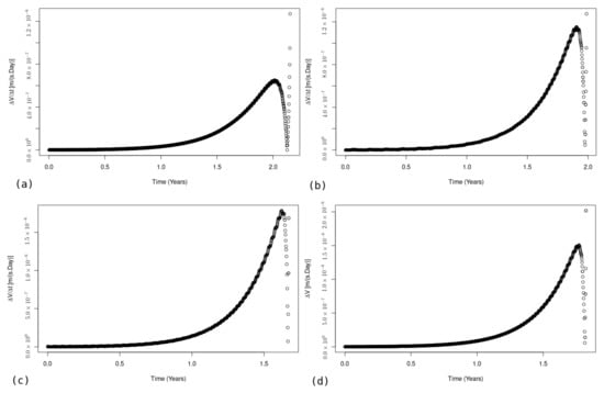
Figure 14.
Magnitude of the impulse per unit of time, in [m/(s. Day)], for relocating the probe to its original circular polar orbit. Each point on the graph corresponds to a time when the maneuver can be performed and the impulse required for it. (a) ; (b) ; (c) ; (d) .
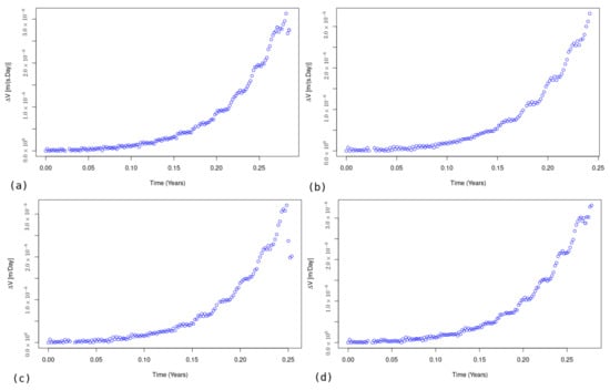
Figure 15.
Magnitude of the impulse per unit of time, in [m/(s. Day)], for reloting the probe to its original circular polar orbit. Each point on the graph corresponds to a time when the maneuver can be performed and the impulse required for it. (a) ; (b) ; (c) ; and (d) .
Figure 14 and Figure 15 show the results for the total impulse required per unit of the time to perform the maneuvers to relocate the probes into their initial circular orbits. The orbits in Figure 14 are the ones with the longest lifetimes, and Figure 15 show the orbits with the lowest lifetimes obtained. The results show that as time progresses, the cost of the impulse to carry out the mission increases, showing that it is more efficient and less costly to perform the maneuver moments before the end of the life of the orbit. It is best to perform the maneuvers at times near the end of the orbits’ lifetime. However, the maneuvers can also be performed in the middle of the entire life of the orbits, which would already produce an increase of at least 50% in the lifetime of the orbits.
These results are interesting because they can be extended to circular orbits with other initial inclinations, with the goal of favoring the accomplishment of possible missions, increasing the lifetime of orbits, and reducing costs related to propellants for station-relocating maneuvers.
4. Final Remarks
In this work, we study the dynamics of natural orbits around the natural satellite Titan. The effects due to Saturn’s gravitational attraction were considered, along with the perturbative effects of non-sphericity of Titan, represented by to the gravitational coefficient . Due to the atmosphere present on Titan, the effects due to atmospheric drag were also considered in this study.
Considering the aforementioned perturbative effects, several grids of initial conditions were simulated, ( and ), for the orbit of the spacecraft with the objective of generating lifetime maps that would allow us to obtain an understanding of the behavior of orbits and locating the regions with the best conditions for carrying out future missions around Titan. These results reinforce the importance and feasibility of studying natural orbits for space probe missions close to natural satellites and other possible systems. In our work, we presented two criteria for the simulations for a possible loss of the probe that showed to have validity and good precision according to the objectives that can be proposed for studies and simulations. The results obtained in the simulations were presented in terms of lifetime maps that showed that, for all cases of initial eccentricities used, there are intervals for the initial inclination of the orbit of the probe, for several intervals of initial semi-major axis, which generate orbits lasting for the total integration time of 20 years. These conditions lie between the initial inclinations of [0.0–50.0]° and [120.0–130.0]°. For inclinations between [50.0–120.0]°, the orbits did not survive the simulation time used, producing orbits with varying durations between a few days and less than 20 years. The results also showed that the orbits with longer durations were those implemented with initial inclinations closer to the lower and upper limits in the range of [50.0–120.0]°. In terms of the initial altitude of the orbits, the results showed that the lower the initial altitude of the orbit, the longer the duration of the orbits. This behavior was observed for all simulated initial eccentricities.
The simulations considering the effect of the flattening of Titan, , showed that, for certain initial orbital conditions, it is possible to have a balance between the third-body effects from Saturn and the effects due to the of Titan. This balance tends to generate orbits with longer lifetimes. However, this was not the dominant behavior observed. Instead, many of the orbits maintained their lifetimes very close to the results considering only the third-body effects, which shows the dominance of the effect on the dynamics of orbits around Titan.
In the study of the effects due to the atmospheric drag present in Titan, it was observed that, in the two regions defined in our work, the drag acted, in most cases, to favor the reduction of the orbit lifetime and thus contribute to the loss of probe, reducing the durations of possible missions. These results show the importance of considering the effects of drag at the lower altitudes of Titan, as these effects change the scenario of the duration of the orbits, being an essential factor to consider for possible missions.
An imbalance was also seen in relation to the choice of and because, even if the value of the longitude of the node does not present much effect in the lifetimes, a good choice for the pericenter argument can give considerable gains, thus allowing longer mission durations.
The investigation of the oscillation rate of the probe altitude, coefficient , showed that the orbits are implemented with higher initial eccentricities. These coefficients grow, reinforcing that the more eccentric orbits present more significant variations in the probe altitude and the orbital lifetime of the probe. In the simulations considering the coefficient of Titan, it was observed that the altitudes of the probe, in general, are divided into two groups: regions where the action of dampens third-body effects and regions where effects due to contribute with the third body to increase the oscillations in the altitude of the probes’ orbits. In the case of the maps of the coefficient , for the simulations considering the perturbations of Saturn, the non-sphericity of Titan, and the atmospheric drag, the same behaviors were observed. There are many orbits with a larger amplitude of oscillation due to the action of atmospheric drag. Circular orbits were the least affected. These results are significant and exciting, as they show the possibility of implementing natural low-inclination circular orbits or even polar orbits around Titan.
We also proposed to carry out maneuvers for some initial polar orbits to find the best moment to apply them. This aims to minimize fuel costs to return the probe to its initial configuration, thus increasing the duration of the orbits. These results are interesting because they can be extended to circular orbits at other initial inclinations, to favor the accomplishment of possible missions, increasing the lifetime of the orbits, and reducing costs related to propellants. All the results presented in this work can help plan missions to Titan, thus contributing to the achievement of the scientific objectives already mentioned in this work.
Author Contributions
Conceptualization, L.S.F., R.S. and A.F.B.A.P.; methodology, L.S.F., R.S. and A.F.B.A.P.; software, L.S.F. and R.S.; formal analysis, L.S.F., R.S. and A.F.B.A.P.; writing—preparation of original draft, L.S.F.; writing—review and editing, L.S.F., R.S. and A.F.B.A.P.; visualization, L.S.F., R.S. and A.F.B.A.P.; supervision, A.F.B.A.P. and R.S. All authors have read and agreed to the published version of the manuscript.
Funding
This study was financed by the Brazilian Federal Agency for Support and Evaluation of Graduate Education (CAPES)-Finance Code 001, and in the scope of the Program CAPES-PrInt, process number 88887.310463/2018-00, International Cooperation Project number 3266. Fundação de Amparo à Pesquisa do Estado de São Paulo (FAPESP)-Proc. 2016/24561-0 and Proc. 2019/23963-5, Conselho Nacional de Desenvolvimento Científico e Tecnológico (CNPq)-Proc. 309089/2021-2. This paper has been supported by the RUDN University Strategic Academic Leadership Program.
Institutional Review Board Statement
Not applicable.
Informed Consent Statement
Not applicable.
Data Availability Statement
All data generated or analyzed during this study are included in this published article in the form of figures.
Acknowledgments
The authors thank The Brazilian Federal Agency for Support and Evaluation of Graduate Education (CAPES)-Finance Code 001, and in the scope of the Program CAPES-PrInt, process number 88887.310463/2018-00, International Cooperation Project number 3266, Fundação de Amparo à Pesquisa do Estado de São Paulo (FAPESP)-Proc. 2016/24561-0 and Proc. 2019/23963-5, Conselho Nacional de Desenvolvimento Científico e Tecnológico (CNPq)-Proc. 309089/2021-2. R.S. also acknowledges support by the Deutsche Forschungsgemeinschaft (DFG)-Project 446102036. This paper has been supported by the RUDN University Strategic Academic Leadership Program.
Conflicts of Interest
The authors declare that they have no conflict of interest in terms of research institutions, professionals, researchers, and/or financial supports.
References
- Kuiper, G.P. Titan: A satellite with an atmosphere. Astrophys. J. 1944, 100, 378. [Google Scholar] [CrossRef]
- Lindal, G.F.; Wood, G.; Hotz, H.; Sweetnam, D.; Eshleman, V.; Tyler, G. The atmosphere of Titan: An analysis of the Voyager 1 radio occultation measurements. Icarus 1983, 53, 348–363. [Google Scholar] [CrossRef]
- Mitchell, J.L.; Lora, J.M. The climate of Titan. Annu. Rev. Earth Planet. Sci. 2016, 44, 353–380. [Google Scholar] [CrossRef]
- Hayes, A.G.; Lorenz, R.D.; Lunine, J.I. A post-Cassini view of Titan’s methane-based hydrologic cycle. Nat. Geosci. 2018, 11, 306–313. [Google Scholar] [CrossRef]
- Hayes, A.G. The lakes and seas of Titan. Annu. Rev. Earth Planet. Sci. 2016, 44, 57–83. [Google Scholar] [CrossRef]
- Lorenz, R.D.; Turtle, E.P.; Barnes, J.W.; Trainer, M.G.; Adams, D.S.; Hibbard, K.E.; Sheldon, C.Z.; Zacny, K.; Peplowski, P.N.; Lawrence, D.J.; et al. Dragonfly: A rotorcraft lander concept for scientific exploration at Titan. Johns Hopkins APL Tech. Dig. 2018, 34, 14. [Google Scholar]
- Spitzer, L. The stability of the 24 hr satellite. J. Br. Interplanet. Soc. 1950, 9, 131. [Google Scholar]
- Kozai, Y. On the Effects of the Sun and the Moon upon the motion of a close Earth satellite. SAO Spec. Rep. 1963, 22. Available online: https://adsabs.harvard.edu/pdf/1959SAOSR..22....2K (accessed on 11 May 2022).
- Blitzer, L. Lunar-solar perturbations of an earth satellite. Am. J. Phys. 1959, 27, 634–645. [Google Scholar] [CrossRef]
- Kaula, W.M. Development of the lunar and solar disturbing functions for a close satellite. Astron. J. 1962, 67, 300. [Google Scholar] [CrossRef]
- De Almeida Prado, A.F.B. Third-body perturbation in orbits around natural satellites. J. Guid. Control Dyn. 2003, 26, 33–40. [Google Scholar] [CrossRef]
- Carvalho, J.d.S.; De Moraes, R.V.; Prado, A. Some orbital characteristics of lunar artificial satellites. Celest. Mech. Dyn. Astron. 2010, 108, 371–388. [Google Scholar] [CrossRef]
- Carvalho, J.; Elipe, A.; De Moraes, R.V.; Prado, A. Low-altitude, near-polar and near-circular orbits around Europa. Adv. Space Res. 2012, 49, 994–1006. [Google Scholar] [CrossRef]
- Domingos, R.d.C.; de Moraes, R.V.; de Almeida Prado, A. Third-body perturbation in the case of elliptic orbits for the disturbing body. Math. Probl. Eng. 2008, 2008, 763654. [Google Scholar] [CrossRef]
- Broucke, R.A. Long-term third-body effects via double averaging. J. Guid. Control. Dyn. 2003, 26, 27–32. [Google Scholar] [CrossRef]
- Murison, M.A. The fractal dynamics of satellite capture in the circular restricted three-body problem. Astron. J. 1989, 98, 2346–2359. [Google Scholar] [CrossRef]
- Carvalho, J.d.S.; Elipe, A.; de Moraes, R.V.; Prado, A. Planetary Satellite Orbiters: Applications for the Moon. Math. Probl. Eng. 2011, 2011, 187478. [Google Scholar] [CrossRef]
- Lara, M.; San-Juan, J.F.; López, L.M.; Cefola, P.J. On the third-body perturbations of high-altitude orbits. Celest. Mech. Dyn. Astron. 2012, 113, 435–452. [Google Scholar] [CrossRef]
- Laskar, J.; Boué, G. Explicit expansion of the three-body disturbing function for arbitrary eccentricities and inclinations. Astron. Astrophys. 2010, 522, A60. [Google Scholar] [CrossRef]
- Liu, X.; Baoyin, H.; Ma, X. Long-term perturbations due to a disturbing body in elliptic inclined orbit. Astrophys. Space Sci. 2012, 339, 295–304. [Google Scholar] [CrossRef]
- Dos Santos, J.C.; Carvalho, J.P.; Prado, A.F.; de Moraes, R.V. Lifetime maps for orbits around Callisto using a double-averaged model. Astrophys. Space Sci. 2017, 362, 227. [Google Scholar] [CrossRef]
- Cinelli, M.; Ortore, E.; Circi, C. Long lifetime orbits for the observation of Europa. J. Guid. Control Dyn. 2019, 42, 123–135. [Google Scholar] [CrossRef]
- Massarweh, L.; Cappuccio, P. On the Restricted 3-Body Problem for the Saturn-Enceladus system: Mission geometry & orbit design for plume sampling missions. In Proceedings of the AIAA Scitech 2020 Forum, Orlando, FL, USA, 6–10 January 2020. [Google Scholar] [CrossRef]
- Waite, J.; Bell, J.; Lorenz, R.; Achterberg, R.; Flasar, F. A model of variability in Titan’s atmospheric structure. Planet. Space Sci. 2013, 86, 45–56. [Google Scholar] [CrossRef]
- Date, S.G.E.; Date, E.M. Titan Atmospheric Modeling Working Group Final Report. 2020. Available online: https://pds-atmospheres.nmsu.edu/data_and_services/atmospheres_data/Cassini/logs/Titan_Atmospheric_Modeling_Working_Group_Final_Report_23_Mar_2020_v3.pdf (accessed on 28 October 2021).
- Murray, C.D.; Dermott, S.F. Solar System Dynamics; Cambridge University Press: Cambridge, UK, 1999. [Google Scholar]
- Rein, H.; Liu, S.F. REBOUND: An open-source multi-purpose N-body code for collisional dynamics. Astron. Astrophys. 2012, 537, A128. [Google Scholar] [CrossRef]
- Everhart, E. An efficient integrator that uses Gauss-Radau spacings. In International Astronomical Union Colloquium; Cambridge University Press: Cambridge, UK, 1985; Volume 83, pp. 185–202. [Google Scholar] [CrossRef][Green Version]
- Rein, H.; Spiegel, D.S. IAS15: A fast, adaptive, high-order integrator for gravitational dynamics, accurate to machine precision over a billion orbits. Mon. Not. R. Astron. Soc. 2015, 446, 1424–1437. [Google Scholar] [CrossRef]
- Marchal, C.L. Fifth John V. Breakwell memorial lecture: The restricted three-body problem revisited. Acta Astronaut. 2000, 47, 411–418. [Google Scholar] [CrossRef]
- Liu, L.; Wang, X. On the orbital lifetime of high-altitude satellites. Chin. Astron. Astrophys. 2000, 24, 284–288. [Google Scholar] [CrossRef]
- Xavier, J.; Prado, A.B.; Winter, S.G.; Amarante, A. Mapping Long-Term Natural Orbits about Titania, a Satellite of Uranus. Symmetry 2022, 14, 667. [Google Scholar] [CrossRef]
- Yelle, R.; Strobel, D.; Lellouch, E.; Gautier, D. Engineering models for Titan’s atmosphere. Huygens Sci. Payload Mission 1997, 1177, 243–256. Available online: https://www.lpl.arizona.edu/~yelle/eprints/Yelle97b.pdf (accessed on 28 October 2021).
- Rodriguez, S.; Vinatier, S.; Cordier, D.; Tobie, G.; Achterberg, R.K.; Anderson, C.M.; Badman, S.V.; Barnes, J.W.; Barth, E.L.; Bézard, B.; et al. Science goals and new mission concepts for future exploration of Titan’s atmosphere, geology and habitability: Titan POlar scout/orbitEr and in situ lake lander and DrONe explorer (POSEIDON). Exp. Astron. 2022, 1–63. [Google Scholar] [CrossRef]
- Nesvornỳ, D.; Alvarellos, J.L.; Dones, L.; Levison, H.F. Orbital and collisional evolution of the irregular satellites. Astron. J. 2003, 126, 398. [Google Scholar] [CrossRef]
Publisher’s Note: MDPI stays neutral with regard to jurisdictional claims in published maps and institutional affiliations. |
© 2022 by the authors. Licensee MDPI, Basel, Switzerland. This article is an open access article distributed under the terms and conditions of the Creative Commons Attribution (CC BY) license (https://creativecommons.org/licenses/by/4.0/).