On Spectral Characterization of Two Classes of Unicycle Graphs

Abstract

Let G be a graph with n vertices, let $A\left(G\right)$ be an adjacency matrix of G and let $P_A(G,\lambda )$ be the characteristic polynomial of $A\left(G\right)$. The adjacency spectrum of G consists of eigenvalues of $A\left(G\right)$. A graph G is said to be determined by its adjacency spectrum (DS for short) if other graphs with the same adjacency spectrum as G are isomorphic to G. In this paper, we investigate the spectral characterization of unicycle graphs with only two vertices of degree three. We use $G_{21}(s_1,s_2)$ to denote the graph obtained from $Q(s_1,s_2)$ by identifying its pendant vertex and the vertex of degree two of $P_3$, where $Q(s_1,s_2)$ is the graph obtained by identifying a vertex of $C_{s_1}$ and a pendant vertex of $P_{s_2}$. We use $G_{31}(t_1,t_2)$ to denote the graph obtained from circle with the vertices $v_0{v}_1\cdots v_{t_1+t_2+1}$ by adding one pendant edge at vertices $v_0$ and $v_{t_1+1}$, respectively. It is shown that $G_{21}(s_1,s_2)$ ($s_1\ne 4,6$, $s_1\ge 3$, $s_2\ge 3$) and $G_{31}(t_1,t_2)$ ($t_1+t_2\ne 2$, $t_2\ge t_1\ge 1$) are determined by their adjacency spectrum.

1. Introduction

All graphs considered here are finite and simple. Undefined notations and terminologies will conform to those in [1].

For a graph G with $n\left(G\right)$ vertices and $m\left(G\right)$ edges, we denote by $V\left(G\right)$ the vertex set and by $E\left(G\right)$ the edge set of G. Let $d_G\left(v\right)$ be the degree of vertex v in G. By $G-v$ and $G-e$ we denote the graphs obtained from G by deleting the vertex v and the edge e. Let G and H be two graphs, we denote by $G\cup H$ the disjoint union of G and H and by $mH$ the disjoint union of m copies of H. We denote by $P_n$ and $C_n$ the path and the cycle with n vertices, respectively. For $n\ge 2$ and $t\ge 3$, we write $\mathcal{P}=\left\{P_n\right|n\ge 2\}$ and $\mathcal{C}=\left\{C_t\right|t\ge 3\}$. Let $T(l_1,l_2,l_3)$ denote a tree with a vertex v of degree three such that $T(l_1,l_2,l_3)-v=P_{l_1}\cup P_{l_2}\cup P_{l_3}$, write ${\mathcal{T}}_1=\left\{T(l_1,l_2,l_3)\right|1\le l_1\le l_2\le l_3\}$.

For a graph G with n vertices, using $A\left(G\right)$ denotes the adjacency matrix of G. The order of $A\left(G\right)$ is n. The element $(i,j)$ of $A\left(G\right)$ is equal to 1 if vertices i and j are adjacent and equal to 0 otherwise. Denote by $P_A(G,\lambda )$ the characteristic polynomial of the adjacency matrix $A\left(G\right)$, which is $|\lambda I-A(G\left)\right|$ a polynomial function of $\lambda$ with degree n. Since $A\left(G\right)$ is a real symmetric matrix, its eigenvalues are all real numbers. Therefore, we assume that ${\lambda }_1\left(G\right)\ge {\lambda }_2\left(G\right)\ge \cdots \ge {\lambda }_n\left(G\right)$ are the adjacency eigenvalues. The multiset of eigenvalues of $A\left(G\right)$ is called the adjacency spectrum of G. The maximum eigenvalue of $A\left(G\right)$ is called the index of G. Two graphs are said to be cospectral with respect to the adjacency matrix if they have the same adjacency spectrum. A graph is said to be determined by its adjacency spectrum (DS for short) if there is no other non-isomorphic graph with the same spectrum with respect to the adjacency matrix.

The authors in [2,3,4] investigated the cospectrality of graphs up to order 11 and provided a survey on spectral characterizations of graphs. In particular, [5,6] have shown that the unicycle graphs with only one vertex of degree three (lollipop graph) are determined by their adjacency spectrum. The authors in [7,8,9] provided some DS-graphs of nearly regular bicyclic graphs with two vertices of the maximum degree three, that is, $\theta$-graphs and dumbbell graphs, where $\theta$-graph (by $\theta (i,j,k)$) is a graph consisting of two given vertices joined by three paths whose order is $i+2$, $j+2$ and $k+2$, respectively, with any two of these paths having only the given vertices in common. The dumbbell graph (by $D(a,b,c)$) consisted of two vertex-disjoint cycles $C_a$, $C_b$ and a path $P_{c+1}$, joining only its end-vertices that were in common with the cycles. Many graphs with special structures have been proved to be determined by their spectrum; see [10,11,12,13,14,15,16].

The structure of a molecule is important for chemists, which can be regarded as a simple graph. For a molecule, the atoms can be replaced by vertices of a graph and the bonds between the atoms and the atoms themselves can be replaced by the edges of a graph. It is convenient to use the adjacency matrices of graphs to denote molecules. Recently, there has been a lot of research on molecular alignment, such as [17,18,19,20]. In [21], the authors introduced two invariants ${\mathsf{\Pi }}_1\left(G\right)$ and ${\mathsf{\Pi }}_2\left(G\right)$ and provided a method to find DS graphs. In this paper, by applying the method, we investigate the spectral characterization of unicycle graphs with only two vertices of the maximum degree three. The necessary and sufficient condition for $G_{21}(s_1,s_2)$ and $G_{31}(t_1,t_2)$ to be DS shall be given, where $G_{21}(s_1,s_2)$ and $G_{31}(t_1,t_2)$ are exhibited in Figure 1.

Figure 1. $G_{21}(s_1,s_2)$ and $G_{31}(t_1,t_2)$.

2. Some Lemmas

For a graph G, $P_A(G,\lambda )={\displaystyle \sum _{k=0}^n}{b}_k\left(G\right){\lambda }^{n-k}$ is the characteristic polynomial of G. In this section, we provide some basic lemmas.

Lemma 1

([22]). Let G be a graph consisting of components $G_1,G_2,\cdots ,G_k$. Then

$$P_A(G,\lambda )=\prod _{i=1}^k{P}_A(G_i,\lambda ).$$

Lemma 2

([22]). Let G be a graph with the vertex v and the edge e. Denote by $\mathcal{C}\left(v\right)\left(\mathcal{C}\right(e\left)\right)$ the set of all cycles in G containing a vertex v (resp. an edge $e=uv$). Then, we have

(i) $P_A(G,\lambda )=\lambda P_A(G-v,\lambda )-{\displaystyle \sum _{u\sim v}}{P}_A(G-\{u,v\},\lambda )-2{\sum }_{C\in \mathcal{C}\left(v\right)}{P}_A(G-V\left(C\right),\lambda ).$

(ii)$P_A(G,\lambda )=P_A(G-uv,\lambda )-P_A(G-\{u,v\},\lambda )-2{\sum }_{C\in \mathcal{C}\left(e\right)}{P}_A(G-V\left(C\right),\lambda ).$

Lemma 3

([21]). Let G be a graph with n vertices. Then

(i) $b_3\left(G\right)=-2N_G\left(K_3\right)$,

(ii) $-b_6\left(G\right)=\frac{m(m^2+3m+4)}{6}-\frac{m+2}{2}{\displaystyle \sum _{i=1}^n}{d}_i^2+\frac{1}{3}{\displaystyle \sum _{i=1}^n}{d}_i^3+{\displaystyle \sum _{ij\in E\left(G\right)}}{d}_i{d}_j-N_G\left(K_3\right)-2N_G(K_2\cup C_4)-4N_G(K_3\cup K_3)+2N_G\left(C_6\right)$.

Write $-b_6\left(G\right)=b_6^{\prime }\left(G\right)+\alpha \left(G\right)$, where $b_6^{\prime }\left(G\right)={\displaystyle \sum _{ij\in E\left(G\right)}}{d}_i{d}_j+2N_G\left(C_6\right)$ and $\alpha \left(G\right)=\frac{m(m^2+3m+4)}{6}-\frac{m+2}{2}{\displaystyle \sum _{i=1}^n}{d}_i^2+\frac{1}{3}{\displaystyle \sum _{i=1}^n}{d}_i^3-N_G\left(K_3\right)-2N_G(K_2\cup C_4)-4N_G(K_3\cup K_3)$.

In [21], we introduced two invariants related to some coefficients of characteristic polynomials of G. One can find the following results from [21].

Definition 1

([21]). Let G be a graph, the parameter ${\mathsf{\Pi }}_1\left(G\right)$ is defined by the following

$${\mathsf{\Pi }}_1\left(G\right)=\left\{\begin{array}{cc}0,\hfill & if m\left(G\right)=0,\hfill \\ b_4\left(G\right)-\left(\begin{array}{c}m\left(G\right)-1\\ 2\end{array}\right)+1,\hfill & if m\left(G\right)>0.\hfill \end{array}\right.$$

Definition 2

([21]). Let G be a connected graph. Set ${\mathsf{\Pi }}_2\left(G\right)={\mathsf{\Pi }}_1\left(G\right)+m\left(G\right)-n\left(G\right)$.

Lemma 4

([21]). (i) Let G and H be two graphs such that $P_A(G,\lambda )=P_A(H,\lambda )$. Then

$${\mathsf{\Pi }}_i\left(G\right)={\mathsf{\Pi }}_i\left(H\right),i=1,2.$$

(ii) Let G be a graph with k components $G_1,G_2,\cdots ,G_k$. Then

$${\mathsf{\Pi }}_2\left(G\right)=\sum _{i=1}^k{\mathsf{\Pi }}_2\left(G_i\right).$$

Lemma 5

([21]). Let G be a connected graph. Then

(i) ${\mathsf{\Pi }}_2\left(G\right)\le 0$, and the equality holds if and only if $G\in \mathcal{P}\cup \mathcal{C}\setminus \left\{C_4\right\}$.

(ii) All connected graphs with $-2\le {\mathsf{\Pi }}_2\left(G\right)\le 0$ are given in Table 1.

Table 1. Graphs with ${\mathsf{\Pi }}_2\left(G\right)=0,-1,-2$.

${\mathbf{\Pi }}_2\left(\mathit{G}\right)$	Graphs
0	$P_n$, $C_3$, $C_n$ for $n\ge 5$
−1	$K_1$, $G_1$, $T_1$
−2	$G_2$, $G_3$, $G_4$, $G_5$, $C_4$, $T_2$

Notice: $G_i$, for $1\le i\le 5$, does not contain $C_4$ as a subgrpah. All dotted lines of graphs in Figure 1 denote a path with at least 2 vertices.

Lemma 6

([22]). All roots of $P_A(C_n,\lambda )$ and $P_A(P_n,\lambda )$ are the following:

$P_A(C_n,\lambda ):2cos\frac{2i\pi }{n},i=0,1,\cdots ,n-1.$

$P_A(P_n,\lambda ):2cos\frac{i\pi }{n+1},i=1,\cdots ,n.$

Let $\lambda =2cos\theta$, set $t^{1/2}=e^{i\theta }$, then it is useful to write the characteristic polynomial of $C_n$ and $P_n$ in the following form:

(1) $P_{C_n}(t^{1/2}+t^{-1/2})=t^{n/2}+t^{-n/2}-2$,

(2) $P_{P_n}(t^{1/2}+t^{-1/2})=t^{-n/2}(t^{n+1}-1)/(t-1)$.

Lemma 7

([22]). Let H be a proper subgraph of a connected graph G, ${\lambda }_1\left(H\right)<{\lambda }_1\left(G\right)$.

Lemma 8

([22]). For a graph G of n vertices with $v\in V\left(G\right)$, let $H=G-v$, then

$${\lambda }_1\left(G\right)\ge {\lambda }_1\left(H\right)\ge {\lambda }_2\left(G\right)\ge {\lambda }_2\left(H\right)\ge \cdots \ge {\lambda }_{n-1}\left(H\right)\ge {\lambda }_n\left(G\right).$$

Lemma 9

([22]). The list of all connected graphs with an index of less than two includes precisely the following graphs: (1) $P_n$ for $n\ge 1$;

(2) $T(a,b,c)$ for $(a,b,c)\in \left\{\right(1,2,2),(1,2,3),(1,2,4\left)\right\}\cup \left\{\right(1,1,n\left)\right|n\ge 1\}$.

3. Main Results

For convenience, we denote by ${\mathcal{G}}_i$ the set $\left\{G_i\right\}$, for $1\le i\le 5$, and by ${\mathcal{T}}_i$ the set $\left\{T_i\right\}$, for $i=1,2$. In this section, we shall show that $G_{21}(s_1,s_2)$ without $C_4$ and $C_6$ as its subgraphs and $G_{31}(t_1,t_2)$ without $C_4$ as its subgraph are DS with respect to their adjacency spectrum.

Lemma 10.

Let H be a graph with $m\left(H\right)=m\left(G_{21}(s_1,s_2)\right)=m\left(G_{31}\right)$ and $n=n\left(H\right)=n\left(G_{21}(s_1,s_2)\right)=n\left(G_{31}\right)$, we have

(i) if $H=H_1\cup H_2$, $H_i\in {\mathcal{G}}_1$, then $b_6^{\prime }\left(H\right)\ge 4n+6$, the equality holds if and only if $H=Q(s_1,2)\cup Q(s_2,2)$, where $s_1\ge 3,s_2\ge 3$, $n=s_1+s_2+2$ and $s_i\ne 6,i=1,2$.

(ii) if $H\in {\mathcal{G}}_2\cup {\mathcal{G}}_3$, then $b_6^{\prime }\left(H\right)\ge 4n+6$, the equality holds if and only if $H\in \{G_{21}(s_1,s_2),G_{31}(t_1,t_2)\}$ and H does not contain $C_6$ as its subgraphs, where $s_1\ge 3$, $t_2\ge t_1\ge 1$, $s_1\ne 6$ and $t_1+t_2\ne 4$.

(iii) if $H\in \{G_4\bigcup P_d,G_5\bigcup P_d\}$, then $b_6^{\prime }\left(H\right)>4n+6$, where $d\ge 2$.

Proof. 

For a graph G with $uv\in E\left(G\right)$, $d_{\times }\left(uv\right)=d_G\left(u\right)\times d_G\left(v\right)$ is said to be the product degree of the edge $uv$. We denote by $D_{\times }\left(G\right)$ the product degree sequence of G, that is, $D_{\times }\left(G\right)=\{d_{\times }\left(e_1\right),d_{\times }\left(e_2\right),\cdots ,d_{\times }\left(e_m\right)\}$, where $E\left(G\right)=\{e_1,e_2,\cdots ,e_m\}$. Now we prove the lemma by considering the product degree sequence of H.

(i) Let $H=H_1\cup H_2$ and $H_i\in {\mathcal{G}}_1$. Then $D_{\times }\left(H\right)$ takes the following cases: $\{3^2,6^4,4^{n-6}\}$, $\{2^1,3^1,6^5,4^{n-7}\}$ and $\{2^2,6^6,4^{n-8}\}$, where $a^k$ in the sets means that H has k edges of the product degree a. Clearly, ${\displaystyle \sum _{uv\in E\left(H\right)}}d\left(u\right)\times d\left(v\right)$ attain the minimum value $4n+6$ if and only if $D_{\times }\left(H\right)=\{3^2,6^4,4^{n-6}\}$. Therefore, by Lemma 3(ii), $b_6^{\prime }\left(H\right)\ge 4n+6$ with the equality holding if and only if $D_{\times }\left(H\right)=\{3^2,6^4,4^{n-6}\}$, which implies $H=Q(s_1,2)\cup Q(s_2,2)$ and $s_i\ne 6,i=1,2$. Thereefore, (i) is true.

(ii) Let $H\in {\mathcal{G}}_2\cup {\mathcal{G}}_3$. To observe all distinct product degree sequences of a graph in ${\mathcal{G}}_2\cup {\mathcal{G}}_3$, one can find that ${\displaystyle \sum _{uv\in E\left(H\right)}}d\left(u\right)\times d\left(v\right)$ attains the minimum value $4n+6$ if and only if $D_{\times }\left(H\right)=\{3^2,6^4,4^{n-6}\}$, which implies $H\in \{G_{21}(s_1,s_2),G_{31}(t_1,t_2)\}$. By Lemma 3(ii), (ii) holds.

With a complete similar argument with that of (i) and (ii), one can prove that (iii) is true. □

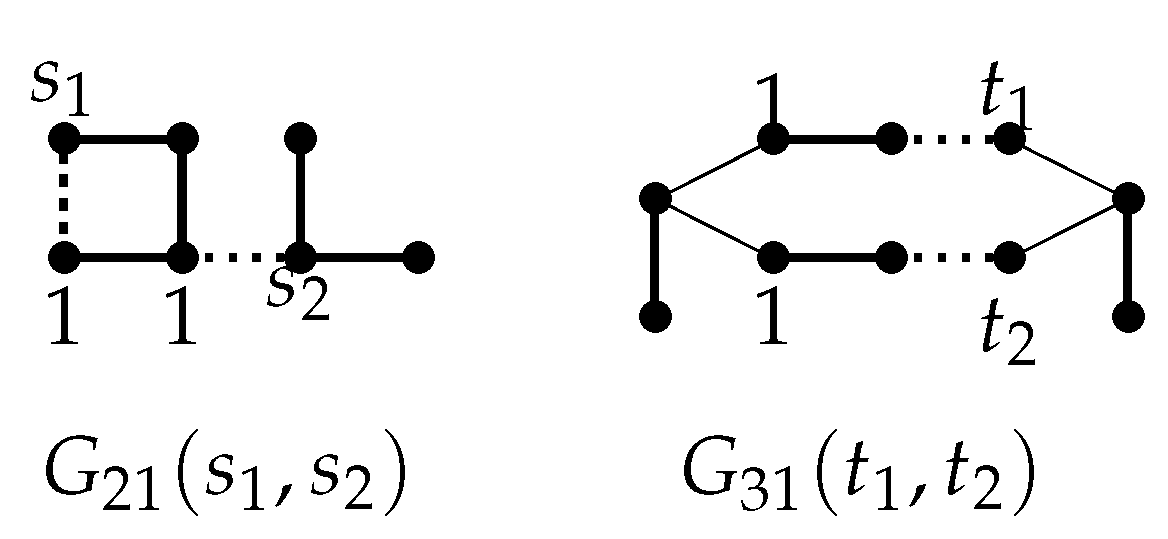
Lemma 11.

Let $s_1\ge 3,s_2\ge 3$ and $n=s_1+s_2+3$. Then $G_{31}(t_1,t_2)$, where $1\le t_1\le t_2,t_1+t_2\ne 2$ and $n=t_1+t_2+4$, is not cospectral with $G_{21}(s_1,s_2)$.

Proof. 

By Lemmas 1 and 2, the characteristic polynomials of $G_{21}(s_1,s_2)$ can be computed as follows:

$P_A\left(G_{21}(s_1,s_2)\right)=\lambda P_A\left(C_{s_1+2}\right)(P_A\left(P_{s_2}\right)-P_A\left(P_{s_2-2}\right))-\lambda P_A\left(P_{s_1+1}\right)(P_A\left(P_{s_2-1}\right)-P_A\left(P_{s_2-3}\right)).$

From Lemma 6, we can write $P_A\left(G_{21}(S_1,S_2)\right)$ as follows (using Mathematica5.0):

$$P_A(G_{21}(s_1,s_2),t^{1/2}+t^{-1/2})t^{n/2}{(t-1)}^4=\psi \left(t\right)+\varphi \left(G_{21}(s_1,s_2)\right),$$

where $\psi \left(t\right)=1-4t+4t^2+2t^3+2t^{n+1}+4t^{n+2}-4t^{n+3}+t^{n+4}$ and

$$\begin{gathered} \varphi \left(G_{21}(s_1,s_2)\right)=-5t^4+2t^5-2t^{1+\frac{s_1}{2}}+6t^{2+\frac{s_1}{2}}-4t^{3+\frac{s_1}{2}}-4t^{4+\frac{s_1}{2}}+6t^{5+\frac{s_1}{2}}-2t^{6+\frac{s_1}{2}}+t^{2+s_1}- \\ 2t^{3+s_1}+2t^{5+s_1}-t^{6+s_1}-t^{1+s_2}+2t^{2+s_2}-2t^{4+s_2}+t^{5+s_2}-2t^{1+\frac{s_1}{2}+s_2}+6t^{2+\frac{s_1}{2}+s_2}-4t^{3+\frac{s_1}{2}+s_2}- \\ 4t^{4+\frac{s_1}{2}+s_2}+6t^{5+\frac{s_1}{2}+s_2}-2t^{6+\frac{s_1}{2}+s_2}+2t^{2+s_1+s_2}-5t^{3+s_1+s_2}. \end{gathered}$$

Using the same method to deal with the characteristic polynomials of $G_{31}(t_1,t_2)$, we obtain

$$\begin{gathered} \varphi \left(G_{31}(t_1,t_2)\right)=-4t^4+t^6-t^{3+t_1}+2t^{4+t_1}-t^{5+t_1}-2t^{1+\frac{t_1+t_2}{2}}+4t^{2+\frac{t_1+t_2}{2}}+2t^{3+\frac{t_1+t_2}{2}}- \\ 8t^{4+\frac{t_1+t_2}{2}}+2t^{5+\frac{t_1+t_2}{2}}+4t^{6+\frac{t_1+t_2}{2}}-2t^{7+\frac{t_1+t_2}{2}}-t^{3+t_2}+2t^{4+t_2}-t^{5+t_2}+t^{2+t_1+t_2}-4t^{4+t_1+t_2}. \end{gathered}$$

Suppose that $G_{21}(s_1,s_2)$ and $G_{31}(t_1,t_2)$ are cospectral, which gives $\varphi \left(G_{21}(s_1,s_2)\right)=\varphi \left(G_{31}(t_1,t_2)\right)$. We consider the possible largest exponents term of $\varphi \left(G_{21}\right)(s_1,s_2).$ They are $-t^{6+s_1},-2t^{6+\frac{s_1}{2}+s_2}$, $-5t^{s_1+s_2+3}$ and their combinations. All the possible combinations of terms are: $\{-t^{6+s_1}\},$$\{-2t^{6+\frac{s_1}{2}+s_2}\},$ $\{-5t^{s_1+s_2+3}\},$$\{-t^{6+s_1}$, $-2t^{6+\frac{s_1}{2}+s_2}\},$$\{-t^{6+s_1},-5t^{s_1+s_2+3}\},$ $\{-2t^{6+\frac{s_1}{2}+s_2},$$-5t^{s_1+s_2+3}\},$$\{-t^{6+s_1},-2t^{6+\frac{s_1}{2}+s_2},-5t^{s_1+s_2+3}\}.$ The coefficients of the front terms are −1, −2, −5, −3, −6, −7, and −8, respectively.

Case 1: $t_1=t_2>2$. Substituting it into $\varphi \left(G_{31}\right)$, we obtain

${\varphi }_1\left(G_{31}\right):-4t^4+t^6-2t^{1+t_1}+4t^{2+t_1}-4t^{4+t_1}+4t^{6+t_1}-2t^{7+t_1}+t^{2+2t_1}-4t^{4+2t_1}.$

We consider the possible largest exponents term of ${\varphi }_1\left(G_{31}\right).$ They are $-2t^{7+t_1},-4t^{4+2t_1}$ and their combinations. All the possible combinations of terms are: $\{-2t^{7+t_1}\},$ $\{-4t^{4+2t_1}\},$$\{-2t^{7+t_1},-4t^{4+2t_1}\}.$ The coefficients of the front terms are −2, −4 and −6, respectively. It is not difficult to see that the largest exponent terms of $\varphi \left(G_{21}\right)$ and ${\varphi }_1\left(G_{31}\right)$ are the same.

Suppose the largest exponent term of ${\varphi }_2\left(G_{31}\right)$ is $\{-2t^{7+t_1}\}$, which gives $7+t_1>4+2t_1,$ so we obtain $t_1<3,$ which is contradicted with $t_1>2.$ Suppose the largest exponent term of ${\varphi }_2$ is $\{-2t^{7+t_1},-4t^{4+2t_1}\}$, which gives $t_1=3$ and $n\left(G_{31}\right)=10$, which is contradicted with $n>10.$ Suppose that the largest exponent term of ${\varphi }_2\left(G_{31}\right)$ is $\{-4t^{4+2t_1}\}$; there is not a combination in ${\varphi }_1\left(G_{21}\right)$ of which the coefficient is −4. It is a contradiction.

Case 2. If $1\le t_1<t_2$, the possible largest exponent terms of $\varphi \left(G_{31}\right)$ are $-t^{5+t_2}$, $-2t^{\frac{t_1+t_2}{2}+7}$, $-4t^{4+t_1+t_2}$ and their combinations. All the possible combinations of terms are: $\{-t^{5+t_2}\},$$\{-2t^{\frac{t_1+t_2}{2}+7}\},$ $\{-4t^{4+t_1+t_2}\},$$\{-t^{5+t_2},-2t^{\frac{t_1+t_2}{2}+7}\},$ $\{-t^{5+t_2},-4t^{4+t_1+t_2}\},$$\{-2t^{\frac{t_1+t_2}{2}+7}$, $-4t^{4+t_1+t_2}\},$$\{-t^{5+t_2},-2t^{\frac{t_1+t_2}{2}+7},-4t^{4+t_1+t_2}\}.$ The coefficients of the front terms are $-1,-2,-4,-3,-5,-6,$ and $-7$, respectively. It is not difficult to see that the largest exponent terms of $\varphi \left(G_{21}\right)$ and $\varphi \left(G_{31}\right)$ are the same. We consider the following possible cases:

Subcase 2.1. Suppose that the largest exponent term of $\varphi \left(G_{31}\right)$ is $\{-t^{5+t_2}\}$. This gives $5+t_2>4+t_1+t_2,$ so we obtain $t_1<1,$ which is contradicted with $t_1\ge 1.$ Suppose that the largest exponent term of $\varphi \left(G_{31}\right)$ is $\{-2t^{\frac{t_1+t_2}{2}+7}\}$. This gives $\frac{t_1+t_2}{2}+7>4+t_1+t_2,$ so we obtain $t_1+t_2<6.$ Since $t_1+t_2>4$, we obtain $t_1+t_2=5$ and $n\left(G_{31}\right)=t_1+t_2+4=9$, which is contradicted with $n>10.$ Suppose that the largest exponent term of $\varphi \left(G_{31}\right)$ is $\{-t^{5+t_2},-2t^{\frac{t_1+t_2}{2}+7}\}$. This gives $\frac{t_1+t_2}{2}+6=5+t_2>4+t_1+t_2,$ so we obtain $t_1<1,$ which is contradicted with $t_1\ge 1.$ Suppose that the largest exponent term of $\varphi \left(G_{31}\right)$ is $\{-4t^{4+t_1+t_2}\}$; there is not a combination in $\varphi \left(G_{21}\right)$ of which the coefficient is −4. It is a contradiction.

Subcase 2.2. Suppose that the largest exponent term of $\varphi \left(G_{31}\right)$ is $\{-t^{5+t_2}$, $-4t^{4+t_1+t_2}\}$, which gives $5+t_2=4+t_1+t_2>\frac{t_1+t_2}{2}+7$ and the coefficient of it is −5. We obtain $t_1=1,t_2>5.$ At the same time, the largest exponent term of ${\varphi }_1\left(G_{21}\right)$ is $\{-5t^{s_1+s_2+3}\}$. It is obviously $s_1+s_2+3=5+t_2$, so $s_2=t_2+2-s_1.$ Substitute $t_2=3$ into ${\varphi }_2$, subtracting the same terms from $\varphi \left(G_{21}\right)$ and $\varphi \left(G_{31}\right)$ simultaneously. We obtain

$$\begin{gathered} {\varphi }_1\left(G_{21}\right):-2t^{1+\frac{s_1}{2}}+6t^{2+\frac{s_1}{2}}-4t^{3+\frac{s_1}{2}}-4t^{4+\frac{s_1}{2}}+6t^{5+\frac{s_1}{2}}-2t^{6+\frac{s_1}{2}}+t^{2+s_1}-2t^{3+s_1}+2t^{5+s_1}-t^{6+s_1}-t^{1+s_2}+2t^{2+s_2}-2t^{4+s_2}+ \\ {t}^{5+s_2}-2t^{1+\frac{s_1}{2}+s_2}+6t^{2+\frac{s_1}{2}+s_2}-4t^{3+\frac{s_1}{2}+s_2}-4t^{4+\frac{s_1}{2}+s_2}+6t^{5+\frac{s_1}{2}+s_2}-2t^{6+\frac{s_1}{2}+s_2} \end{gathered}$$

${\varphi }_2\left(G_{31}\right):-2t^{\frac{t_2+3}{2}}+4t^{\frac{t_2+5}{2}}+2t^{\frac{t_2+7}{2}}-8t^{\frac{t_2+9}{2}}+2t^{\frac{t_2+11}{2}}+4t^{\frac{t_2+13}{2}}-2t^{\frac{t_2+15}{2}}.$

The largest exponent term of ${\varphi }_1\left(G_{21}\right)$ is $-2t^{\frac{t_2+15}{2}}.$ The largest exponent term of ${\varphi }_1\left(G_{21}\right)$ may be $-t^{6+s_1},-2t^{6+\frac{s_1}{2}+s_2}$ and their combinations. However, the coefficient which equals −2 is only $-2t^{6+\frac{s_1}{2}+s_2}$. Therefore, we obtain $\frac{t_2+15}{2}=6+\frac{s_1}{2}+s_2$, then $s_1+2s_2=t_2+3$. Since $s_1+s_2=t_2+2$, we obtain $s_2=1$, which is contradicted with $s_2\ge 3.$

Subcase 2.3. Suppose that the largest exponent term of $\varphi \left(G_{31}\right)$ is $\{-2t^{\frac{t_1+t_2}{2}+7},-4t^{4+t_1+t_2}\},$ which gives $\frac{t_1+t_2}{2}+7=4+t_1+t_2>5+t_2$, and the coefficient of it is −6. We obtain $t_1+t_2=6.$ At the same time, the largest exponent term of $\varphi \left(G_{21}\right)$ is $\{-t^{6+s_1},-5t^{s_1+s_2+3}\}$. It is obviously $6+s_1=s_1+s_2+3>6+\frac{s_1}{2}+s_2$, so we obtain $s_1>6,s_2=3$. We also know that $6+s_1=t_1+t_2+4=10$, so $s_1=4$, which is contradicted with $s_1>6.$

Subcase 2.4. Suppose that the largest exponent term of $\varphi \left(G_{31}\right)$ is $\{-t^{5+t_2},$$-2t^{\frac{t_1+t_2}{2}+7}$, $-4t^{4+t_1+t_2}\}$, which gives $5+t_2=\frac{t_1+t_2}{2}+7=4+t_1+t_2$ and the coefficient of it is −7. We obtain $t_1=1,t_2=5.$ At the same time, the largest exponent term of $\varphi \left(G_{21}\right)$ is $\{-2t^{6+\frac{s_1}{2}+s_2},-5t^{s_1+s_2+3}\}$. It is obviously $6+\frac{s_1}{2}+s_2=s_1+s_2+3>6+s_1$, so we obtain $s_1=6,s_2>3$. We also know that $9+s_2=t_1+t_2+4=10$, so $s_2=1$, which is contradicted with $s_2>3.$ Then, we complete the proof of Lemma 11. □

Lemma 12.

(i) Let $s_1\ge 3,s_2\ge 3$ and $t_1\ge 3,t_2\ge 3$. If $s_1+s_2=t_1+t_2$, then $G_{21}(s_1,s_2)$ and $G_{21}(t_1,t_2)$ are cospectral if and only if $s_1=t_1$ and $s_2=t_2$.

(ii) Let $s_2\ge s_1\ge 1$ and $t_2\ge t_1\ge 1$. If $s_1+s_2=t_1+t_2$, then $G_{31}(s_1,s_2)$ and $G_{31}(t_1,t_2)$ are cospectral if and only if $s_1=t_1$ and $s_2=t_2$.

Proof. 

(i) Suppose that $G_{21}(s_1,s_2)$ and $G_{21}(t_1,t_2)$ are cospectral, which gives $\varphi \left(G_{21}(s_1,s_2)\right)=\varphi \left(G_{21}(t_1,t_2)\right)$. Similarly with $\varphi \left(G_{21}(s_1,s_2)\right)$, one can easily obtain

$$\begin{gathered} \varphi \left(G_{21}(t_1,t_2)\right)=-5t^4+2t^5-2t^{1+\frac{t_1}{2}}+6t^{2+\frac{t_1}{2}}-4t^{3+\frac{t_1}{2}}-4t^{4+\frac{t_1}{2}}+6t^{5+\frac{t_1}{2}}-2t^{6+\frac{t_1}{2}}+ \\ {t}^{2+t_1}-2t^{3+t_1}+2t^{5+t_1}-t^{6+t_1}-t^{1+t_2}+2t^{2+t_2}-2t^{4+t_2}+t^{5+t_2}-2t^{1+\frac{t_1}{2}+t_2}+6t^{2+\frac{t_1}{2}+t_2}- \\ 4t^{3+\frac{t_1}{2}+t_2}-4t^{4+\frac{t_1}{2}+t_2}+6t^{5+\frac{t_1}{2}+t_2}-2t^{6+\frac{t_1}{2}+t_2}+2t^{2+t_1+t_2}-5t^{3+t_1+t_2}. \end{gathered}$$

By eliminating the same terms of $\varphi \left(G_{21}(s_1,s_2)\right)$ and $\varphi \left(G_{21}(t_1,t_2)\right)$, we obtain

$$\begin{gathered} {\varphi }_1\left(G_{21}(s_1,s_2)\right):-2t^{1+\frac{s_1}{2}}+6t^{2+\frac{s_1}{2}}-4t^{3+\frac{s_1}{2}}-4t^{4+\frac{s_1}{2}}+6t^{5+\frac{s_1}{2}}-2t^{6+\frac{s_1}{2}}+t^{2+s_1}-2t^{3+s_1}+2t^{5+s_1}-t^{6+s_1}-t^{1+s_2}+2t^{2+s_2}- \\ 2t^{4+s_2}+t^{5+s_2}-2t^{1+\frac{s_1}{2}+s_2}+6t^{2+\frac{s_1}{2}+s_2}-4t^{3+\frac{s_1}{2}+s_2}-4t^{4+\frac{s_1}{2}+s_2}+6t^{5+\frac{s_1}{2}+s_2}-2t^{6+\frac{s_1}{2}+s_2}, \end{gathered}$$

$$\begin{gathered} {\varphi }_1\left(G_{21}(t_1,t_2)\right):-2t^{1+\frac{t_1}{2}}+6t^{2+\frac{t_1}{2}}-4t^{3+\frac{t_1}{2}}-4t^{4+\frac{t_1}{2}}+6t^{5+\frac{t_1}{2}}-2t^{6+\frac{t_1}{2}}+t^{2+t_1}-2t^{3+t_1}+2t^{5+t_1}-t^{6+t_1}-t^{1+t_2}+2t^{2+t_2}- \\ 2t^{4+t_2}+t^{5+t_2}-2t^{1+\frac{t_1}{2}+t_2}+6t^{2+\frac{t_1}{2}+t_2}-4t^{3+\frac{t_1}{2}+t_2}-4t^{4+\frac{t_1}{2}+t_2}+6t^{5+\frac{t_1}{2}+t_2}-2t^{6+\frac{t_1}{2}+t_2}. \end{gathered}$$

The smallest possible terms of ${\varphi }_1\left(G_{21}(s_1,s_2)\right)$ are $-2t^{1+\frac{s_1}{2}}$, $-t^{1+s_2}$ and their combination $\{-2t^{1+\frac{s_1}{2}},-t^{1+s_2}\}$. The smallest possible terms of ${\varphi }_1\left(G_{21}(t_1,t_2)\right)$ are $-2t^{1+\frac{t_1}{2}}$, $-t^{1+t_2}$ and their combination $\{-2t^{1+\frac{t_1}{2}},-t^{1+t_2}\}$. The coefficients of the front terms are −2, −1 and −3.

Case 1. Suppose the smallest term of ${\varphi }_1\left(G_{21}(s_1,s_2)\right)$ is $-2t^{1+\frac{s_1}{2}}$. Since ${\varphi }_1\left(G_{21}(s_1,s_2)\right)={\varphi }_1\left(G_{21}(t_1,t_2)\right)$, we can easily obtain the smallest term of ${\varphi }_1\left(G_{21}(t_1,t_2)\right)$, which is $-2t^{1+\frac{t_1}{2}}$, which gives $t_1=s_1$. Substituting it into ${\varphi }_1\left(G_{21}(t_1,t_2)\right)$ and eliminating the same terms of ${\varphi }_1\left(G_{21}(s_1,s_2)\right)$ and ${\varphi }_1\left(G_{21}(t_1,t_2)\right)$, we obtain

${\varphi }_2\left(G_{21}(s_1,s_2)\right):-t^{1+s_2}+2t^{2+s_2}-2t^{4+s_2}+t^{5+s_2}-2t^{1+\frac{s_1}{2}+s_2}+6t^{2+\frac{s_1}{2}+s_2}-4t^{3+\frac{s_1}{2}+s_2}-4t^{4+\frac{s_1}{2}+s_2}+6t^{5+\frac{s_1}{2}+s_2}-2t^{6+\frac{s_1}{2}+s_2},$

${\varphi }_2\left(G_{21}(t_1,t_2)\right):-t^{1+t_2}+2t^{2+t_2}-2t^{4+t_2}+t^{5+t_2}-2t^{1+\frac{s_1}{2}+t_2}+6t^{2+\frac{s_1}{2}+t_2}-4t^{3+\frac{s_1}{2}+t_2}-4t^{4+\frac{s_1}{2}+t_2}+6t^{5+\frac{s_1}{2}+t_2}-2t^{6+\frac{s_1}{2}+t_2}.$

Obviously, the smallest term of ${\varphi }_2\left(G_{21}(s_1,s_2)\right)$ is $-t^{1+s_2}$, and so is $-t^{1+t_2}$ of ${\varphi }_2\left(G_{21}(t_1,t_2)\right)$. Since ${\varphi }_2\left(G_{21}(s_1,s_2)\right)={\varphi }_2\left(G_{21}(t_1,t_2)\right)$, we obtain $t_2=s_2$.

Case 2. Suppose the smallest term of ${\varphi }_1\left(G_{21}(s_1,s_2)\right)$ is $-t^{1+s_2}$ or $\{-2t^{1+\frac{s_1}{2}},-t^{1+s_2}\}$. Similarly to Case 1, we obtain $s_1=t_1$ and $s_2=t_2$. We complete the proof of Lemma 12(i).

(ii) Similarly to the proof of (i), we can easily obtain (ii). Then, we complete the proof of Lemma 12. □

Theorem 1.

Let $s_1\ge 3,s_2\ge 2$. Then $G_{21}(s_1,s_2)$, $s_1\ne 4,6$, is determined by its adjacency spectrum.

Proof. 

Let H be a graph cospectral with $G_{21}(s_1,s_2)$. Without loss of generality, we assume that H has k connected components $H_1$, $H_2$, ⋯, $H_k$. By Lemma 4 and Table 1, it follows that

$${\mathsf{\Pi }}_2\left(H\right)=\sum _{i=1}^k{\mathsf{\Pi }}_2\left(H_i\right)={\mathsf{\Pi }}_2\left(G_{21}(s_1,s_2)\right)=-2.$$

By Lemma 5, it is easy to see that $-2\le {\mathsf{\Pi }}_2\left(H_i\right)\le 0$, for $1\le i\le k$. Therefore, H has exactly one component, say $H_1$, such that ${\mathsf{\Pi }}_2\left(H_1\right)=-2$ and ${\mathsf{\Pi }}_2\left(H_i\right)=0$ for $2\le i\le k$, or H has exactly two components, say $H_1$ and $H_2$, such that ${\mathsf{\Pi }}_2\left(H_1\right)={\mathsf{\Pi }}_2\left(H_1\right)=-1$ and ${\mathsf{\Pi }}_2\left(H_i\right)=0$ for $3\le i\le k$.

Now we observe the largest eigenvalue and the second eigenvalue of $G_{21}(s_1,s_2)$. By Lemmas 6 and 7, we obtain ${\lambda }_1\left(G_{21}(s_1,s_2)\right)>{\lambda }_1\left(C_{s_1+2}\right)=2$. Choose the middle vertex u of degree three of $G_{21}(s_1,s_2)$ such that $G_{21}-u=P_{s_1+1}\cup T(1,1,s_2-2)$. By Lemmas 8 and 9, we obtain ${\lambda }_2\left(G_{21}(s_1,s_2)\right)<2$. Hence, we know that 2 is not the eigenvalue of $G_{21}(s_1,s_2)$, which implies that H does not contain C as its component. Therefore, we distinguish the following cases:

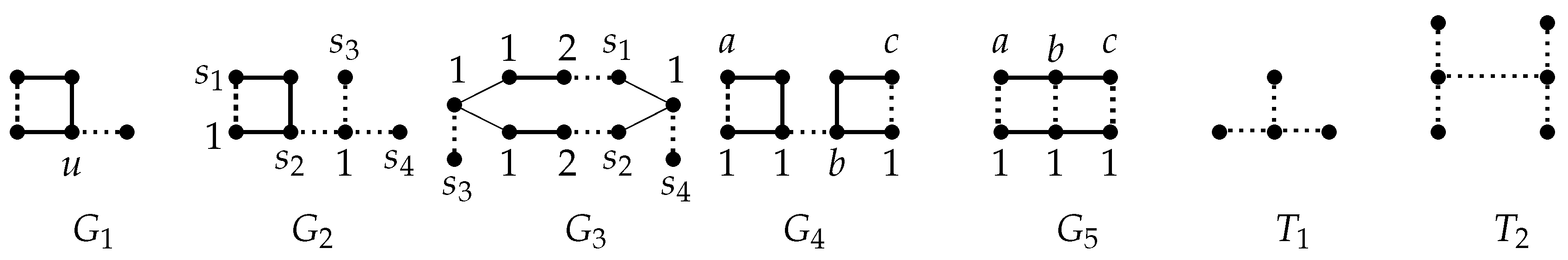
Case 1. ${\mathsf{\Pi }}_2\left(H_1\right)={\mathsf{\Pi }}_2\left(H_1\right)=-1$ and ${\mathsf{\Pi }}_2\left(H_i\right)=0$ for $3\le i\le k$. By Lemma 5, Table 1 and Figure 2,

$$H_1,H_2\in \{K_1,G_1,T_1\},H_i\in \mathcal{P},i=3,\cdots ,k.$$

Clearly, $m\left(H_i\right)\le n\left(H_i\right)$ and $n\left(G_{21}(s_1,s_2)\right)=m\left(G_{21}(s_1,s_2)\right)$, so $k=2$ and $H_1,H_2\in {\mathcal{G}}_1$. Note that ${\lambda }_1\left(H_1\right)>2$ and ${\lambda }_1\left(H_2\right)>2$, which contradict with ${\lambda }_2\left(G_{21}(s_1,s_2)\right)<2$.

Case 2. ${\mathsf{\Pi }}_2\left(H_1\right)=-2$ and ${\mathsf{\Pi }}_2\left(H_i\right)=0$ for $2\le i\le k$. By Lemma 5 and Table 1,

$$H_1\in \{G_2,G_3,G_4,G_5,T_2\},H_i\in \mathcal{P},i=2,3,\cdots ,k$$

and $H_1$ has no subgraphs $C_4$.

Figure 2. All connected graphs with $-2\le {\mathsf{\Pi }}_2\left(G\right)\le 0$.

Clearly, $m\left(H_1\right)=n\left(H_1\right)$ for each $H_1\in \{G_2,G_3\}$; $m\left(H_1\right)=n\left(H_1\right)+1$ for each $H_1\in \{G_4,G_5\}$; $m\left(H_1\right)=n\left(H_1\right)-1$ for $H_1\in \left\{T_2\right\}$ and $m\left(H_i\right)=n\left(H_i\right)-1$ for each $i\ge 2$. Since $m\left(H\right)-n\left(H\right)=m\left(G_{21}\right)-n\left(G_{21}\right)=0$, we arrive at

(i) $H\in \{G_2,G_3\}$, or

(ii) $H=H_1\cup H_2$, where $H_1\in \{G_4,G_5\}$ and $H_2\in \mathcal{P}$.

Suppose that $H\in \{G_2,G_3\}$ and H have no subgraphs $C_4$. Then H and $G_{21}(s_1,s_2)$ have the same degree sequence and number of $K_3$’s. Therefore, by Lemma 3 we obtain that $b_6^{\prime }\left(H\right)=b_6^{\prime }\left(G_{21}(s_1,s_2)\right)=4n+6$ for $s_1\ne 4$. From Lemma 10(ii), we have that $H\in \{G_{21}(t_1,t_2),G_{31}(a,b)\}$ and H does not contain $C_6$ as its subgraphs, where $t_1\ge 3$, $b\ge a\ge 1$, $t_1\ne 4$ and $a+b\ne 4$. By Lemmas 11 and 12(i), we obtain $H=G_{21}(s_1,s_2)$.

Suppose that $H\in \{G_4\bigcup P_d,G_5\bigcup P_d\}$. By Lemma 10(ii), we have $b_6^{\prime }\left(H\right)>4n+6=b_6^{\prime }\left(G_{21}(s_1,s_2)\right)$, which implies $P_A\left(H\right)\ne P_A\left(G_{21}(s_1,s_2)\right)$ from Lemma 3. Therefore, the theorem holds. □

Lemma 13.

Let $s_2\ge s_1\ge 3$ and $n=s_1+s_2+2$. Then, we have $G_{31}(t_1,t_2)$, where $1\le t_1\le t_2,t_1+t_2\ne 2$ and $n=t_1+t_2+4$ is not cospectral with $Q(s_1,2)\cup Q(s_2,2)$.

Proof. 

For convenience, we use F instead of $Q(s_1,2)\cup Q(s_2,2)$. We deal with the characteristic polynomials of F in the same way as Lemma 11. By eliminating the same terms, we obtain

$$\begin{gathered} \varphi \left(G_{31}^{\prime }(t_1,t_2)\right):-t^{3+t_1}+2t^{4+t_1}-t^{5+t_1}-2t^{1+\frac{t_1+t_2}{2}}+4t^{2+\frac{t_1+t_2}{2}}+2t^{3+\frac{t_1+t_2}{2}}-8t^{4+\frac{t_1+t_2}{2}}+2t^{5+\frac{t_1+t_2}{2}}+4t^{6+\frac{t_1+t_2}{2}}-2t^{7+\frac{t_1+t_2}{2}}- \\ {t}^{3+t_2}+2t^{4+t_2}-t^{5+t_2} \end{gathered}$$,

$$\begin{gathered} \varphi \left(F\right):-2t^{\frac{s_1}{2}}+6t^{1+\frac{s_1}{2}}-2t^{2+\frac{s_1}{2}}-8t^{3+\frac{s_1}{2}}+6t^{4+\frac{s_1}{2}}+2t^{5+\frac{s_1}{2}}-2t^{6+\frac{s_1}{2}}+t^{s_1}-2t^{1+s_1}-2t^{2+s_1}+6t^{3+s_1}-2t^{4+s_1}-2t^{5+s_1}+ \\ {t}^{6+s_1}-2t^{\frac{s_2}{2}}+6t^{1+\frac{s_2}{2}}-2t^{2+\frac{s_2}{2}}-8t^{3+\frac{s_2}{2}}+6t^{4+\frac{s_2}{2}}+2t^{5+\frac{s_2}{2}}-2t^{6+\frac{s_2}{2}}+t^{s_2}-2t^{1+s_2}-2t^{2+s_2}+6t^{3+s_2}-2t^{4+s_2}-2t^{5+s_2}+ \\ {t}^{6+s_2}+4t^{\frac{s_1+s_2}{2}}-8t^{1+\frac{s_1+s_2}{2}}-4t^{2+\frac{s_1+s_2}{2}}+16t^{3+\frac{s_1+s_2}{2}}-4t^{4+\frac{s_1+s_2}{2}}-8t^{5+\frac{s_1+s_2}{2}}+4t^{6+\frac{s_1+s_2}{2}}-2t^{\frac{s_1}{2}+s_2}+2t^{1+\frac{s_1}{2}+s_2}+6t^{2+\frac{s_1}{2}+s_2}- \\ 8t^{3+\frac{s_1}{2}+s_2}-2t^{4+\frac{s_1}{2}+s_2}+6t^{5+\frac{s_1}{2}+s_2}-2t^{6+\frac{s_1}{2}+s_2}-2t^{\frac{s_2}{2}+s_1}+2t^{1+\frac{s_2}{2}+s_1}+6t^{2+\frac{s_2}{2}+s_1}-8t^{3+\frac{s_2}{2}+s_1}-2t^{4+\frac{s_2}{2}+s_1}+6t^{5+\frac{s_2}{2}+s_1}- \\ 2t^{6+\frac{s_2}{2}+s_1}. \end{gathered}$$

Case 1. $t_1=t_2>2$. Substituting it into $\varphi \left(G_{31}^{\prime }(t_1,t_2)\right)$, we obtain

${\varphi }_1\left(G_{31}^{\prime }(t_1,t_2)\right):-2t^{1+t_1}+4t^{2+t_1}-4t^{4+t_1}+4t^{6+t_1}-2t^{7+t_1}.$

Obviously, the largest exponent term of ${\varphi }_1\left(G_{31}^{\prime }(t_1,t_2)\right)$ is $-2t^{7+t_1}$ and the smallest exponent term of ${\varphi }_1\left(G_{31}^{\prime }(t_1,t_2)\right)$ is $-2t^{1+t_1}$. The difference of the two exponents is six.

Subcase 1.1. $s_1=s_2>2$. Substituting it into $\varphi \left(F\right)$, we obtain

$$\begin{gathered} {\varphi }_1\left(F\right):-4t^{\frac{s_1}{2}}+12t^{1+\frac{s_1}{2}}-4t^{2+\frac{s_1}{2}}-16t^{3+\frac{s_1}{2}}+12t^{4+\frac{s_1}{2}}+4t^{5+\frac{s_1}{2}}-4t^{6+\frac{s_1}{2}}+6t^{s_1}-12t^{1+s_1}-8t^{2+s_1}+28t^{3+s_1}-8t^{4+s_1}- \\ 12t^{5+s_1}+6t^{6+s_1}-4t^{\frac{3s_1}{2}}+4t^{1+\frac{3s_1}{2}}+12t^{2+\frac{3s_1}{2}}-16t^{3+\frac{3s_1}{2}}-4t^{4+\frac{3s_1}{2}}+12t^{5+\frac{3s_1}{2}}-4t^{6+\frac{3s_1}{2}} \end{gathered}$$.

Obviously, the largest exponent term of ${\varphi }_1\left(F\right)$ is $-4t^{6+\frac{3s_1}{2}}$. The coefficients of the largest term of ${\varphi }_1\left(G_{31}^{\prime }(t_1,t_2)\right)$ and ${\varphi }_1\left(F\right)$ are different, which is a contradiction.

Subcase 1.2. If $s_2>s_1$, one can see the smallest term of $\varphi \left(F\right)$ is $-2t^{\frac{s_1}{2}}$, while the largest term of $\varphi \left(F\right)$ is $-2t^{6+\frac{s_1}{2}+s_2}$. The difference of two exponents is $6+s_2$, which is not six.

Case 2. If $1\le t_1<t_2$, the possible largest exponent terms of $\varphi \left(G_{31}^{\prime }(t_1,t_2)\right)$ are $-t^{5+t_2}$, $-2t^{\frac{t_1+t_2}{2}+7}$ and their combinations. The coefficients of the front terms are −1, −2 and $-3$, respectively. When $s_1=s_2>2$, the coefficient of the largest term of ${\varphi }_1\left(F\right)$ is −4, which does not appear in $\varphi \left(G_{31}^{\prime }(t_1,t_2)\right)$. If $s_2>s_1$, one can see the smallest term of $\varphi \left(F\right)$ is $-2t^{\frac{s_1}{2}}$, while the largest term of $\varphi \left(F\right)$ is $-2t^{6+\frac{s_1}{2}+s_2}$. The difference of two exponents is $6+s_2$. Therefore, the largest term of $\varphi \left(G_{31}^{\prime }(t_1,t_2)\right)$ is $-2t^{\frac{t_1+t_2}{2}+7}$, which gives $\frac{t_1+t_2}{2}+7>5+t_2$. We obtain $t_2<4+t_1$. Thus, the smallest exponent term of ${\varphi }_1\left(G_{31}^{\prime }(t_1,t_2)\right)$ is $-2t^{1+\frac{t_1+t_2}{2}}$. The difference of the two exponents is six. This results in a contradiction. Then, we complete the proof of Lemma 13. □

Lemma 14.

Let $(t_1,t_2)\in \{(4,19),(5,11),(7,7)\}$. Then, we have $G_{31}(t_1,t_2)$, which are not cospectral with $G_{21}(s_1,s_2)\bigcup C_s$ and $G_{31}(a,b)\bigcup C_s$.

Proof. 

$(t_1,t_2)=(4,19)$. Suppose $G_{31}(4,19)$ is cospectral with H, which gives $n\left(H\right)=n\left(G_{31}(4,19)\right)=27$, where $H\in \{G_{21}(s_1,s_2)\bigcup C_s,G_{31}(a,b)\bigcup C_s\}$. It is not hard to see that both the length and the number of shortest odd cycles in $G_{31}(4,19)$ and H are the same. $G_{31}(4,19)$ contains an odd cycle with the length 25, and so does H. Suppose $H=G_{21}(s_1,s_2)\bigcup C_s$, we can easily obtain $s_1=23,s>25$ or $s_1>23,s=25$. Then, we have $n\left(H\right)>27$, which is contradicted with $n\left(G_{31}(4,19)\right)=n\left(H\right)$. Suppose $H=G_{31}(a,b)\bigcup C_s$, we can easily obtain $a+b=23,s>25$ or $a+b>23,s=25$. Then, we have $n\left(H\right)>27$, which is contradicted with $n\left(G_{31}(4,19)\right)=n\left(H\right)$.

$(t_1,t_2)=(5,11)$. Suppose $G_{31}(5,11)$ is cospectral with H, which gives $n\left(H\right)=n\left(G_{31}(5,11)\right)=20$, ${\mathsf{\Pi }}_2\left(H\right)={\mathsf{\Pi }}_2\left(G_{31}(5,11)\right)$ and $b_6^{\prime }\left(H\right)=b_6^{\prime }\left(G_{31}(5,11)\right)$, where $H\in \{G_{21}(s_1,s_2)\bigcup C_s,G_{31}(a,b)\bigcup C_s\}$. $G_{31}(5,11)$ is a biparticle graph, and so is H. Suppose $H=G_{21}(s_1,s_2)\bigcup C_s$, we can easily obtain $s_1=2i,s=2j$, where $i\ge 3,j\ge 4$. Since $n\left(H\right)=s_1+s_2+s+3=20$, one can see $i=3,j=4$ and $H=G_{21}(6,3)\bigcup C_8$. We calculate the eigenvalues of $G_{31}(5,11)$ and $C_8$. The eigenvalues of $G_{31}(5,11)$ are $\{-2.083968,-2,-1.902113,-1.618034,-1.571841,-1.175571,-1,-0.618034,-0.431733,$ $0_2,0.431733,0.618034,1,1.175571,1.571841,1.618034,1.902113,2,2.083968\}.$ The eigenvalues of $C_8$ are $\{-2,-1.{414214}_2,0_2,1.{414214}_2,2\}.$ We can see −1.414214 is a eigenvalue of H; however, it is not a eigenvalue of $G_{31}(5,11)$. This results in a contradiction. Suppose $H=G_{31}(a,b)\bigcup C_s$, we can easily obtain $a+b=2i,s=2j$, where $i\ge 3,j\ge 4$. Since $n\left(H\right)=a+b+s+4=20$, one can see $i=4,j=4$ or $i=3,j=5$. $H=G_{31}(a,b)\bigcup C_8$ or $H=G_{31}(a,b)\bigcup C_{10}$. If $H=G_{31}(a,b)\bigcup C_8$, we arrive at a contradiction. We calculate the eigenvalues of $C_{10}$, which are $\{-2,-{1.618034}_2,-{0.618034}_2,{0.618034}_2,{1.618034}_2,2\}.$ We can see −1.618034 is a eigenvalue of H, with multiplicity at least 2. However, it is a simple eigenvalue of $G_{31}(5,11)$. This results in a contradiction.

$(t_1,t_2)=(7,7)$. Suppose $G_{31}(7,7)$ is cospectral with H, which gives $n\left(H\right)=n\left(G_{31}(7,7)\right)=18$, ${\mathsf{\Pi }}_2\left(H\right)={\mathsf{\Pi }}_2\left(G_{31}(7,7)\right)$ and $b_6^{\prime }\left(H\right)=b_6^{\prime }\left(G_{31}(7,7)\right)$, where $H\in \{G_{21}(s_1,s_2)\bigcup C_s,G_{31}(a,b)\bigcup C_s\}$. $G_{31}(7,7)$ is biparticle graph, and so is H. Suppose $H=G_{21}(s_1,s_2)\bigcup C_s$, we can easily obtain $s_1=2i,s=2j$, where $i\ge 3,j\ge 4$. Since $s_2\ge 3$, $n\left(H\right)=s_1+s_2+s+3\ge 20$. $n\left(H\right)=n\left(G_{31}(7,7)\right)\ne n\left(H\right)$, which a contradiction. Suppose $H=G_{31}(a,b)\bigcup C_s$, we can easily obtain $a+b=2i,s=2j$, where $i\ge 3,j\ge 4$. Since $n\left(G_{31}(7,7)\right)=n\left(H\right)=a+b+s+4=18$, one can see $i=3,j=4$. Thus, $H=G_{31}(a,b)\bigcup C_8$, and we have arrived at a contradiction. Then, we complete the proof of Lemma 14. □

Theorem 2.

Let $1\le t_1\le t_2$ and $t_1+t_2\ne 2$. Then, $G_{31}(t_1,t_2)$ is determined by its adjacency spectrum.

Proof. 

Let H be a graph cospectral with $G_{31}(t_1,t_2)$. Without loss of generality, we assume that H has k connected components $H_1$, $H_2$, ⋯, $H_k$. By Lemma 4 and Table 1, it follows that

$${\mathsf{\Pi }}_2\left(H\right)=\sum _{i=1}^k{\mathsf{\Pi }}_2\left(H_i\right)={\mathsf{\Pi }}_2\left(G_{31}(t_1,t_2)\right)=-2.$$

By Lemma 5, it is easy to see that $-2\le {\mathsf{\Pi }}_2\left(H_i\right)\le 0$, for $1\le i\le k$. Therefore, H has exactly one component, say $H_1$, such that ${\mathsf{\Pi }}_2\left(H_1\right)=-2$ and ${\mathsf{\Pi }}_2\left(H_i\right)=0$ for $2\le i\le k$, or H has exactly two components, say $H_1$ and $H_2$, such that ${\mathsf{\Pi }}_2\left(H_1\right)={\mathsf{\Pi }}_2\left(H_1\right)=-1$ and ${\mathsf{\Pi }}_2\left(H_i\right)=0$ for $3\le i\le k$.

Now, we observe whether two is the root of $P_A\left(G_{31}(t_1,t_2)\right)$ or not. By Lemma 1 and 2, we have $P_A(G_{31}(t_1,t_2),2)=t_1{t}_2-3t_1-3t_2-7$. If two is the root of $P_A\left(G_{31}(t_1,t_2)\right)$, we obtain $t_1=3+\frac{16}{t_2-3}$. $P_A\left(G_{31}(t_1,t_2)\right)$ contains two as its root, if and only if $(t_1,t_2)\in \{(4,19),(5,11),(7,7)\}$. We consider the following case.

Case 1. If $(t_1,t_2)\notin \{(4,19),(5,11),(7,7)\}$, we know that two is not the eigenvalue of $G_{31}(t_1,t_2)$, which implies that H does not contain C as its component. Therefore, we distinguish the following cases:

Subcase 1.1. ${\mathsf{\Pi }}_2\left(H_1\right)={\mathsf{\Pi }}_2\left(H_1\right)=-1$ and ${\mathsf{\Pi }}_2\left(H_i\right)=0$ for $3\le i\le k$. By Lemma 5 and Table 1,

$$H_1,H_2\in \{K_1,G_1,T_1\},H_i\in \mathcal{P},i=3,\cdots ,k.$$

Clearly, $m\left(H_i\right)\le n\left(H_i\right)$ and $n\left(G_{21}(s_1,s_2)\right)=m\left(G_{21}(s_1,s_2)\right)$, so $k=2$ and $H_1,H_2\in {\mathcal{G}}_1$. Suppose that H has no subgraphs $C_4$. Then, H and $G_{31}(t_1,t_2)$ have the same degree sequence and number of $K_3$’s. Therefore, by Lemma 3 we obtain that $b_6^{\prime }\left(H\right)=b_6^{\prime }\left(G_{31}(t_1,t_2)\right)=4n+6$. From Lemma 10 (i), we have that $H=Q(s_1,2)\cup Q(s_2,2)$. By Lemma 13, $G_{31}(t_1,t_2)$ is not cospectral with $Q(s_1,2)\cup Q(s_2,2)$.

Subcase 1.2. ${\mathsf{\Pi }}_2\left(H_1\right)=-2$ and ${\mathsf{\Pi }}_2\left(H_i\right)=0$ for $2\le i\le k$. By Lemma 5 and Table 1,

$$H_1\in \{G_2,G_3,G_4,G_5,T_2\},H_i\in \mathcal{P},i=2,3,\cdots ,k$$

and $H_1$ has no subgraphs $C_4$.

Clearly, $m\left(H_1\right)=n\left(H_1\right)$ for each $H_1\in \{G_2,G_3\}$; $m\left(H_1\right)=n\left(H_1\right)+1$ for each $H_1\in \{G_4,G_5\}$; $m\left(H_1\right)=n\left(H_1\right)-1$ for $H_1\in \left\{T_2\right\}$ and $m\left(H_i\right)=n\left(H_i\right)-1$ for each $i\ge 2$. Since $m\left(H\right)-n\left(H\right)=m\left(G_{31}(t_1,t_2)\right)-n\left(G_{31}(t_1,t_2)\right)=0$, we arrive at

(i) $H\in \{G_2,G_3\}$, or

(ii) $H=H_1\cup H_2$, where $H_1\in \{G_4,G_5\}$ and $H_2\in \mathcal{P}$.

Suppose that $H\in \{G_2,G_3\}$ and H have no subgraphs $C_4$. Then H and $G_{31}(t_1,t_2)$ have the same degree sequence and number of $K_3$’s. Therefore, by Lemma 3 we obtain that $b_6^{\prime }\left(H\right)=b_6^{\prime }\left(G_{31}(t_1,t_2)\right)=4n+6$ for $t_1+t_2\ne 4$. From Lemma 10 (ii), we have that $H\in \{G_{21}(t_1,t_2),G_{31}(a,b)\}$ and H does not contain $C_6$ as its subgraphs, where $t_1\ge 3$, $b\ge a\ge 1$, $t_1\ne 4$ and $a+b\ne 4$. By Lemmas 11 and 12(i), we obtain $H=G_{31}(t_1,t_2)$.

Suppose that $H\in \{G_4\bigcup P_d,G_5\bigcup P_d\}$. By Lemma 10 (ii), we have $b_6^{\prime }\left(H\right)>4n+6=b_6^{\prime }\left(G_{31}(t_1,t_2)\right)$, which implies $P_A\left(H\right)\ne P_A\left(G_{31}(t_1,t_2)\right)$ from Lemma 3. Therefore, in this case, the theorem holds.

Case 2. If $(t_1,t_2)\in \{(4,19),(5,11),(7,7)\}$, we know that 2 is a eigenvalue of $G_{31}(t_1,t_2)$. H may contain C as its component. Now, we observe the largest eigenvalue, the second and third eigenvalue of $G_{31}(t_1,t_2)$. By Lemmas 6 and 7, we obtain ${\lambda }_1\left(G_{31}(t_1,t_2)\right)>{\lambda }_1\left(C_{s_1+2}\right)=2$. Choose the vertex u of degree three of $G_{31}(t_1,t_2)$, such that $G_{31}(t_1,t_2)-u=K_1\cup T(1,t_1,t_2)$. Choose the vertex v of degree three of $T(1,t_1,t_2)$, such that $T(1,t_1,t_2)-v=K_1\cup P_{t_1}\cup P_{t_2}$. By Lemmas 8 and 9, we obtain ${\lambda }_3\left(G_{31}(t_1,t_2)\right)<2$. Hence, we know that $G_{31}(t_1,t_2)$ at most has two eigenvalues, which are not smaller than two. $Q(s_1,2)\cup Q(s_2,2)\bigcup C_s$ has three eigenvalues, which are not larger than two. We have $H\ne Q(s_1,2)\cup Q(s_2,2)\bigcup C_s$. By Lemma 10, we can easily obtain $b_6^{\prime }\left(G_{31}\right)<b_6^{\prime }\left(H\right)$, where $H\in \{\mathcal{C}\bigcup {\mathcal{G}}_i\setminus \{G_{21}(s_1,s_{2}1),G_{31}(t_1,t_2)\},\mathcal{C}\bigcup \mathcal{P}\bigcup {\mathcal{G}}_j|i=2,3;j=4,5\}$. Thus, we just consider $H\in \{G_{21}(s_1,s_2)\bigcup C_s,G_{31}(a,b)\bigcup C_s\}$. By Lemma 14, we have H, which is not cospectral with $G_{31}(t_1,t_2)$. Then, we complete the proof. □