Author Contributions
Data curation, J.R.; formal analysis, J.R., M.A.R., P.L.C. and J.A.; investigation, J.R., M.A.R. and P.L.C.; methodology, J.R., M.A.R., P.L.C. and J.A.; writing—original draft, J.R., M.A.R., P.L.C. and J.A.; writing—review and editing, M.A.R., P.L.C. and J.A.; Funding Acquisition, J.R., M.A.R. and J.A. All authors have read and agreed to the published version of the manuscript.
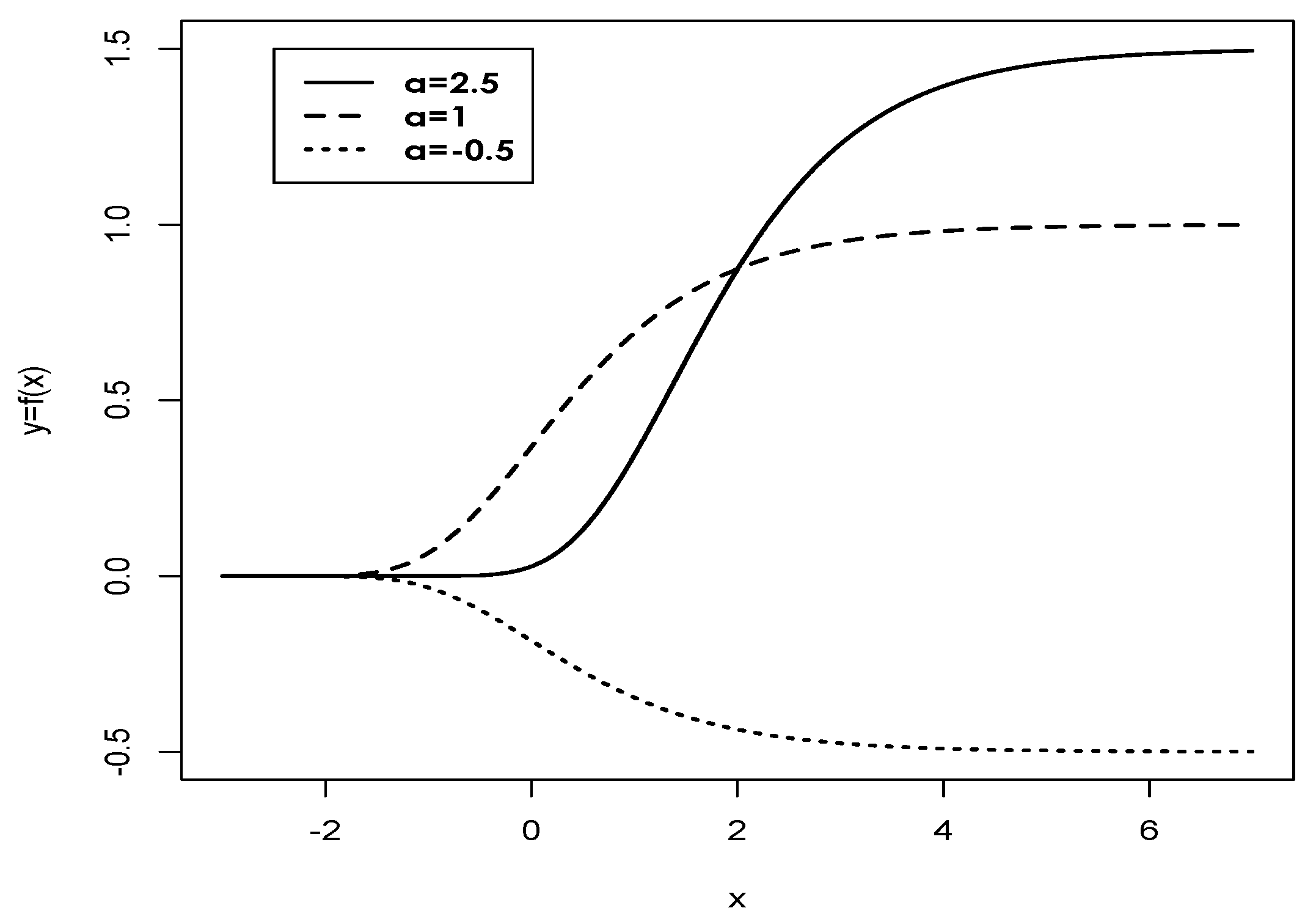
Figure 1.
Plot of Gompertz function for (solid line), (dotted line), (dashed line) and .
Figure 1.
Plot of Gompertz function for (solid line), (dotted line), (dashed line) and .
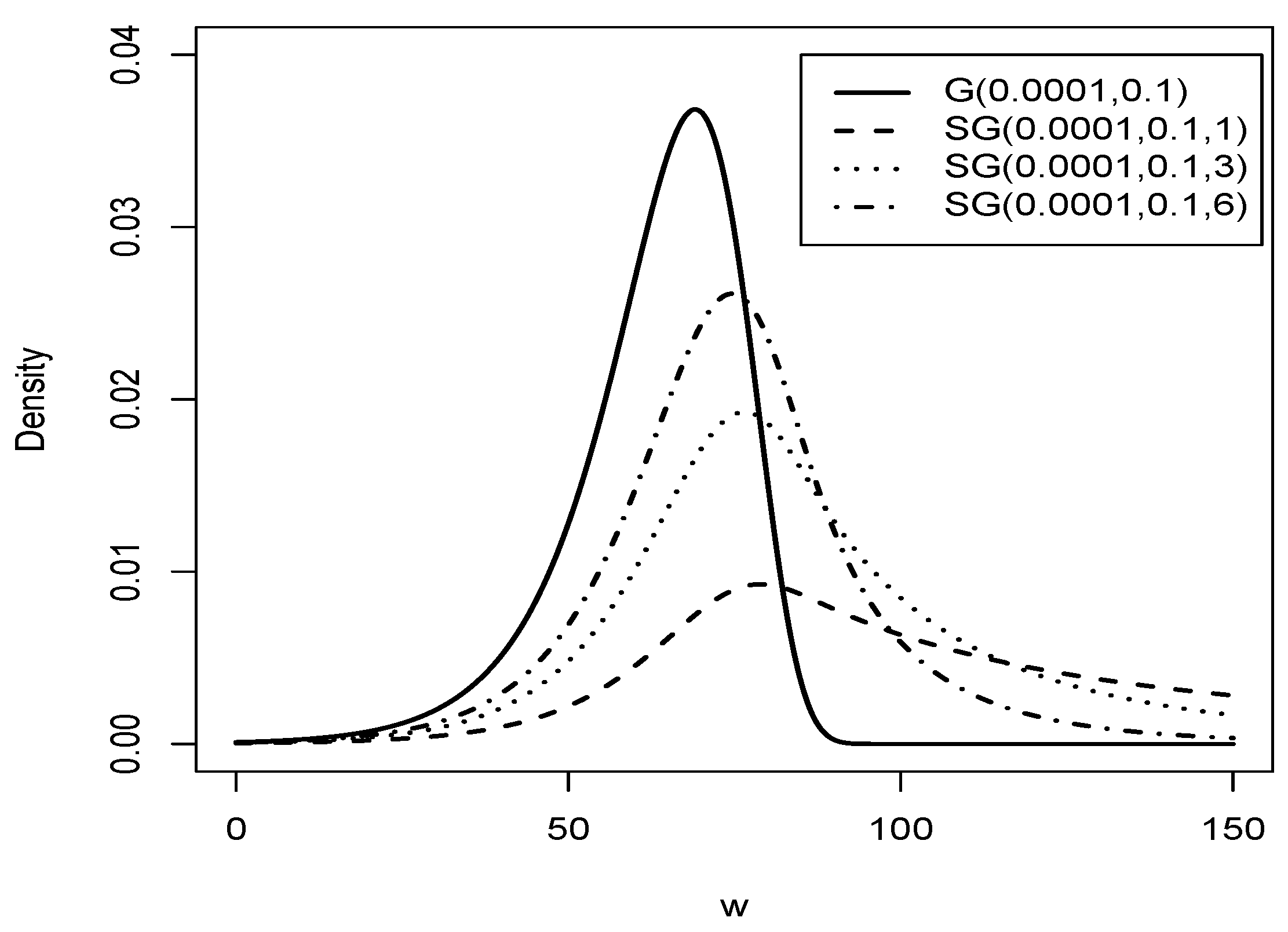
Figure 2.
Graphic of comparison of the G distribution (solid line) with distribution for = 0.0001, = 0.01 and (dashed line), (dotted line), (dashed dotted line).
Figure 2.
Graphic of comparison of the G distribution (solid line) with distribution for = 0.0001, = 0.01 and (dashed line), (dotted line), (dashed dotted line).
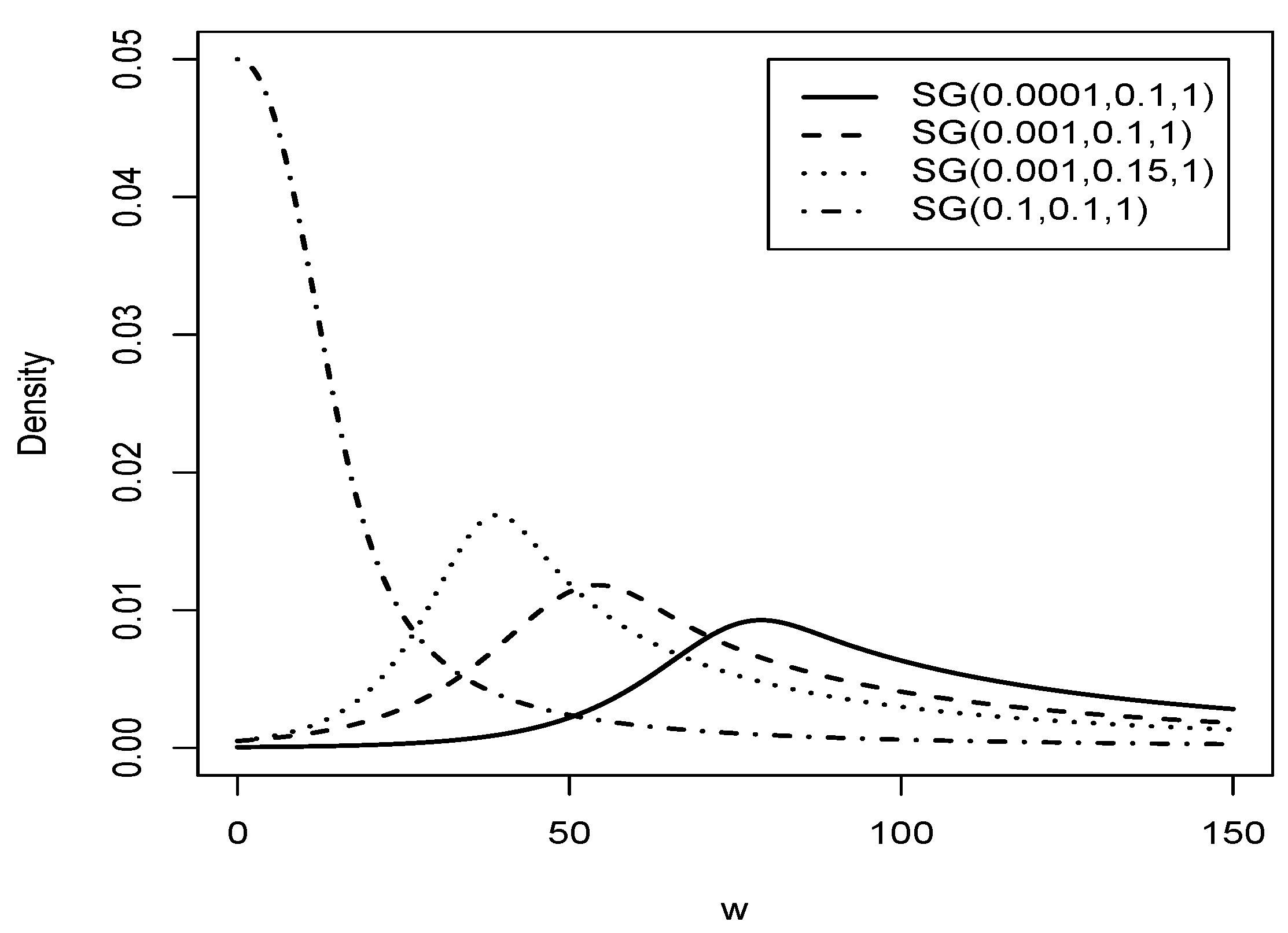
Figure 3.
Graphic comparison of the distribution for and different values of and .
Figure 3.
Graphic comparison of the distribution for and different values of and .
Figure 4.
Cumulative distribution functions for the distributions compared to the G distribution for values of , and q.
Figure 4.
Cumulative distribution functions for the distributions compared to the G distribution for values of , and q.
Figure 5.
Reliability functions for the distributions compared to the G distribution for values of , and .
Figure 5.
Reliability functions for the distributions compared to the G distribution for values of , and .
Figure 6.
The hazard rate functions for the and G distribution.
Figure 6.
The hazard rate functions for the and G distribution.
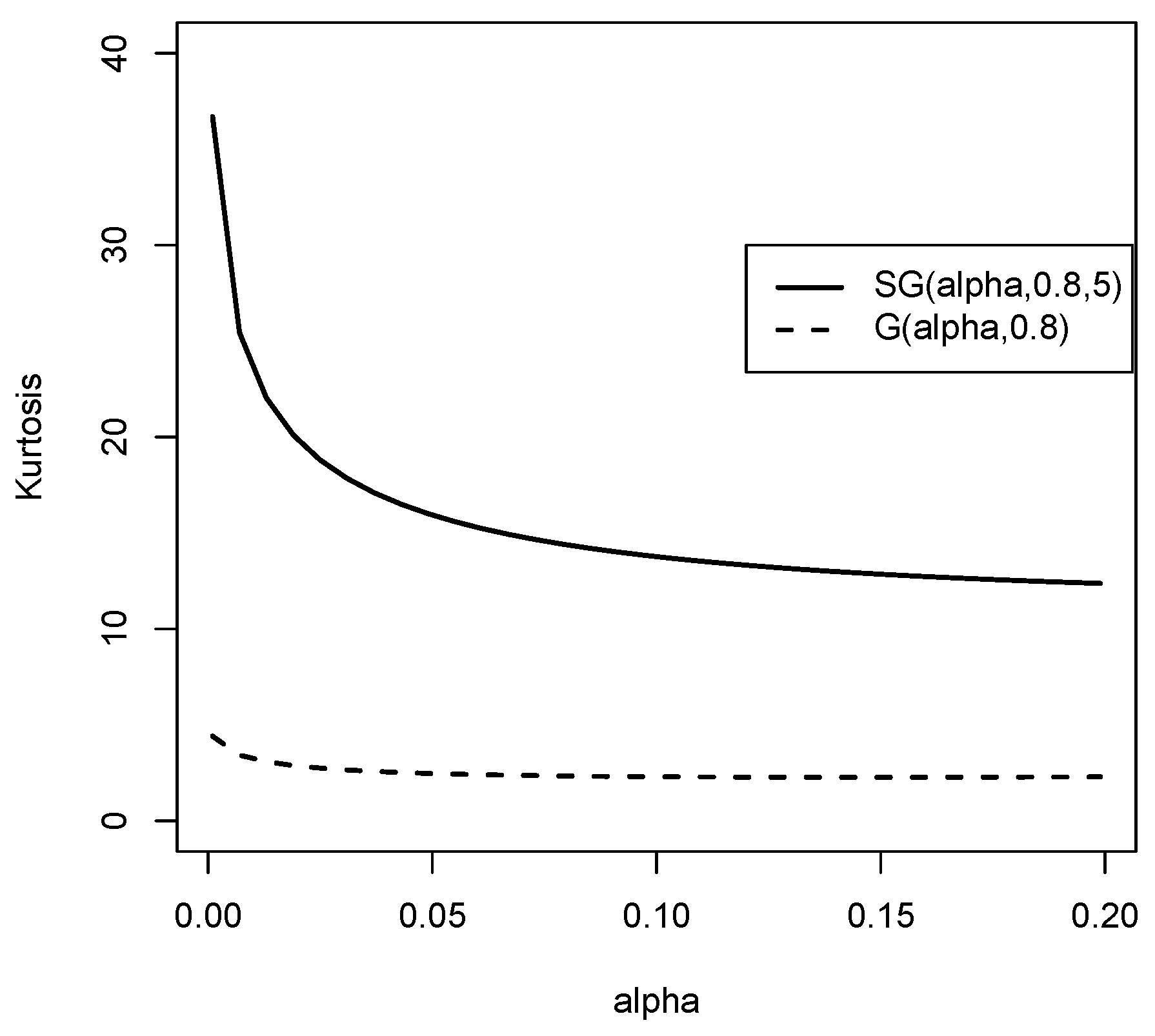
Figure 7.
Kurtosis coefficient graphic for the and the Gompertz distribution.
Figure 7.
Kurtosis coefficient graphic for the and the Gompertz distribution.
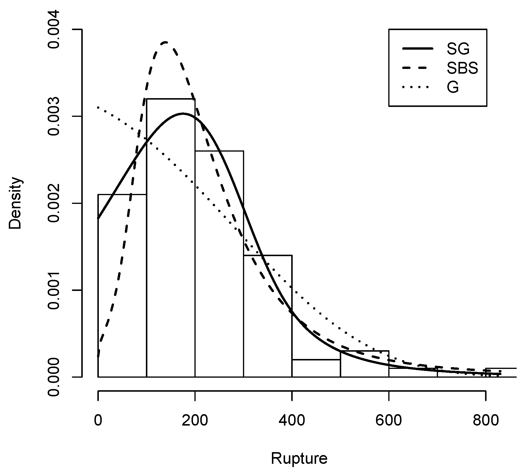
Figure 8.
Rupture data histogram with Density (solid line), G density (dashed line) and density (dotted line).
Figure 8.
Rupture data histogram with Density (solid line), G density (dashed line) and density (dotted line).
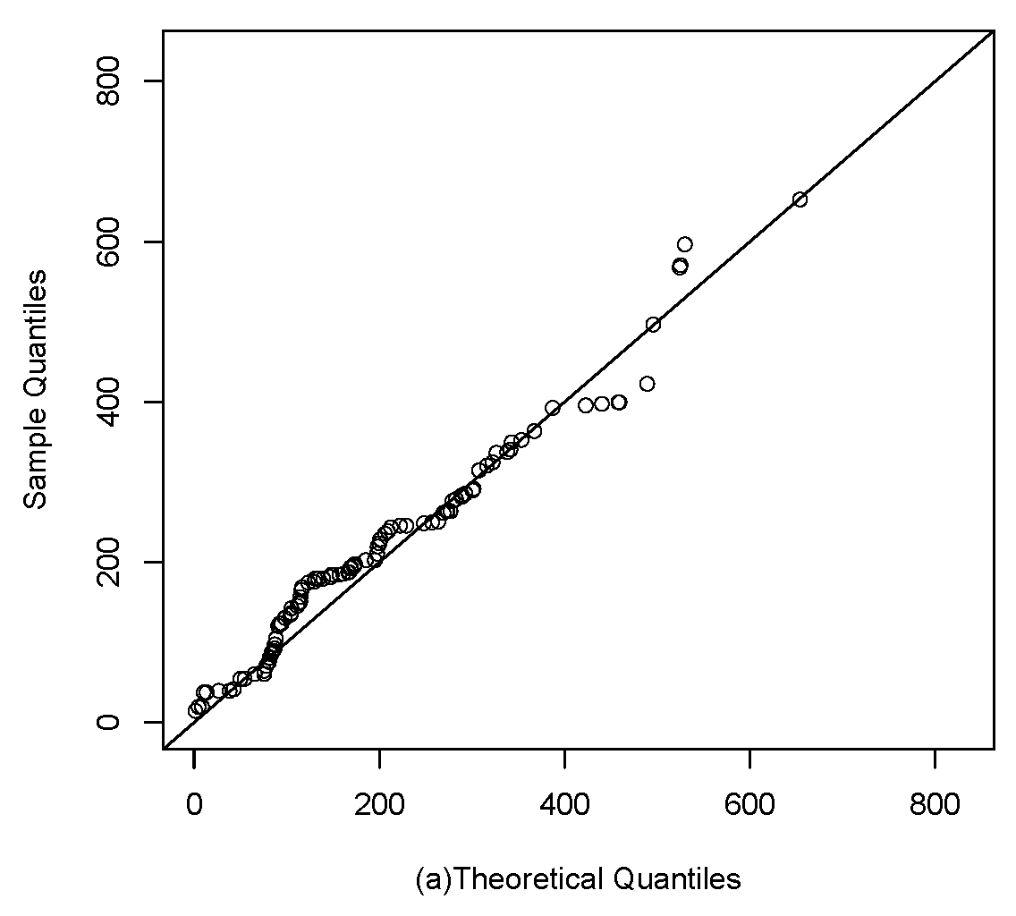
Figure 9.
Q-q plots: (a), (b) and G (c).
Figure 9.
Q-q plots: (a), (b) and G (c).
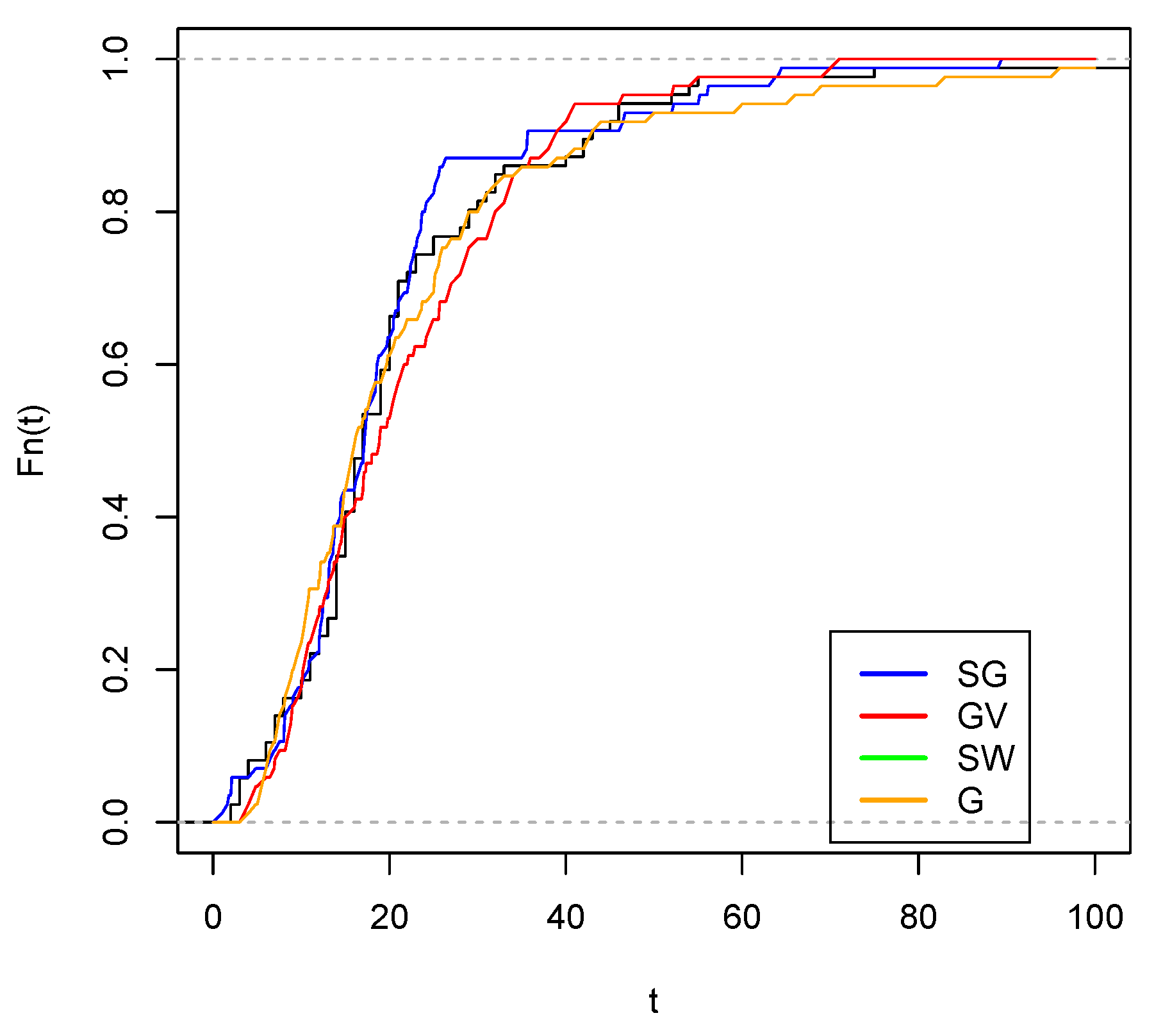
Figure 10.
Empirical cdf with estimated c.d.f. (red color), estimated G c.d.f. (green color) and estimated cdf (blue color).
Figure 10.
Empirical cdf with estimated c.d.f. (red color), estimated G c.d.f. (green color) and estimated cdf (blue color).
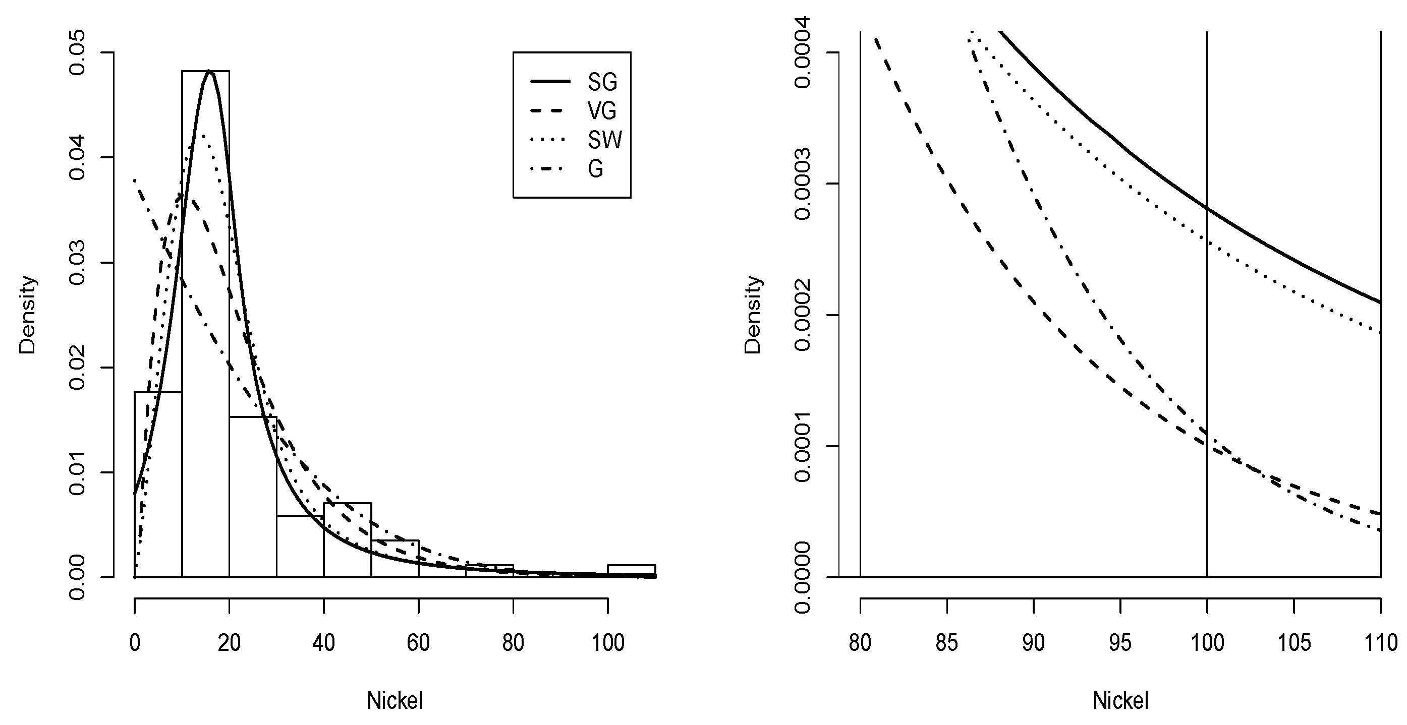
Figure 11.
Data nickel histogram with density (solid line), density (dashed line), density (dotted line) and G density (dashed-dotted line).
Figure 11.
Data nickel histogram with density (solid line), density (dashed line), density (dotted line) and G density (dashed-dotted line).
Figure 12.
Q-q plots: (a), (b) (c) and G (d).
Figure 12.
Q-q plots: (a), (b) (c) and G (d).
Figure 13.
Empirical cdf with estimated G c.d.f. (orange color), c.d.f. (green color), estimated c.d.f. (red color) and estimated cdf (blue color).
Figure 13.
Empirical cdf with estimated G c.d.f. (orange color), c.d.f. (green color), estimated c.d.f. (red color) and estimated cdf (blue color).
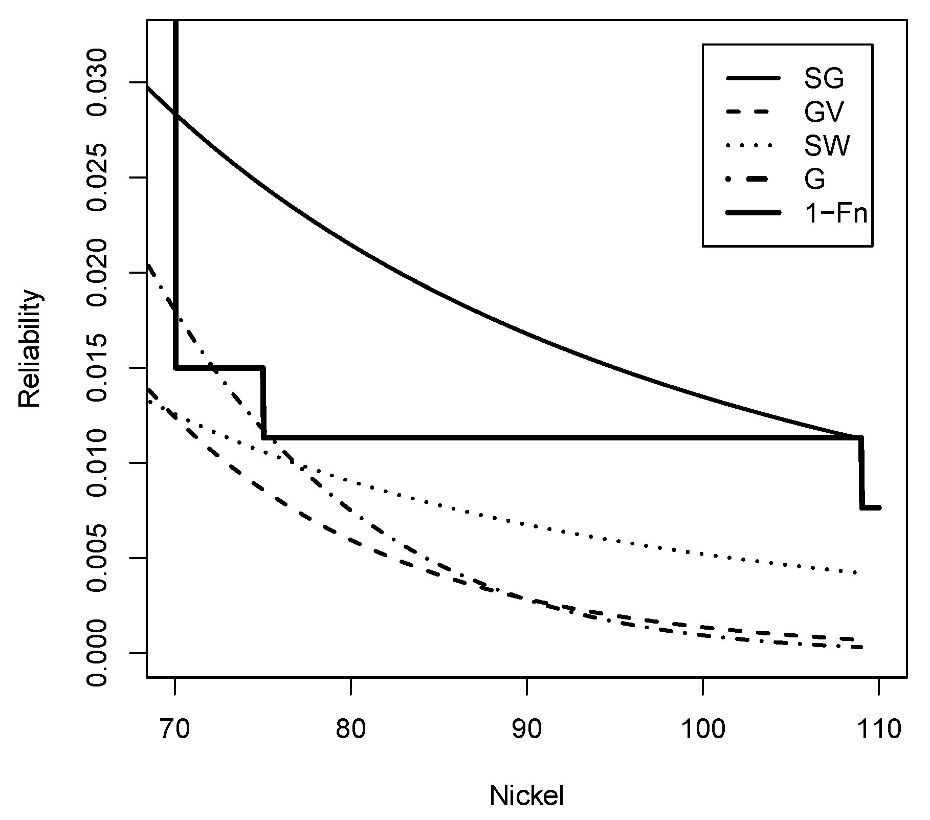
Figure 14.
Reliability function (Solid line), (dashed line), (dotted line), G (dashed-dotted line) and Empirical reliability (Solid Line) for nickel data set.
Figure 14.
Reliability function (Solid line), (dashed line), (dotted line), G (dashed-dotted line) and Empirical reliability (Solid Line) for nickel data set.
Table 1.
Reliability function comparison for distributions of G, and .
Table 1.
Reliability function comparison for distributions of G, and .
| Distribution | | | | | |
|---|
| G | 0.0036 | 0.0014 | 0.0006 | 0.0003 | 0.0001 |
| 0.0260 | 0.0255 | 0.0250 | 0.0240 | 0.0241 |
| 0.4912 | 0.4796 | 0.4685 | 0.4578 | 0.4476 |
Table 2.
Simulation of 2000 iterations of the model .
Table 2.
Simulation of 2000 iterations of the model .
| n | | | q | | | | | | | | | | | | |
|---|
| 50 | 0.3 | 0.8 | 2 | 0.2856 | 0.1097 | 0.4300 | 95.80 | 0.9213 | 0.5182 | 2.0312 | 94.20 | 2.3408 | 0.9507 | 3.7266 | 94.20 |
| 100 | 0.3 | 0.8 | 2 | 0.2970 | 0.0814 | 0.3191 | 95.25 | 0.8320 | 0.3327 | 1.3041 | 95.05 | 2.2171 | 0.6490 | 2.5441 | 94.50 |
| 200 | 0.3 | 0.8 | 2 | 0.2967 | 0.0574 | 0.2252 | 95.35 | 0.8281 | 0.2219 | 0.8700 | 95.10 | 2.0702 | 0.3626 | 1.4215 | 95.05 |
| 500 | 0.3 | 0.8 | 2 | 0.2987 | 0.0367 | 0.1437 | 95.25 | 0.8068 | 0.1330 | 0.5215 | 94.45 | 2.0334 | 0.1891 | 0.7413 | 94.65 |
| 50 | 0.5 | 0.8 | 2 | 0.4674 | 0.1669 | 0.6543 | 95.40 | 1.0022 | 0.6540 | 2.5639 | 93.80 | 2.2997 | 0.9467 | 3.7110 | 94.40 |
| 100 | 0.5 | 0.8 | 2 | 0.4884 | 0.1237 | 0.4849 | 95.25 | 0.8579 | 0.4110 | 1.6110 | 95.30 | 2.2498 | 0.7464 | 2.9260 | 94.95 |
| 200 | 0.5 | 0.8 | 2 | 0.4931 | 0.0886 | 0.3472 | 95.40 | 0.8361 | 0.2822 | 1.1064 | 95.00 | 2.1004 | 0.4795 | 1.8795 | 96.20 |
| 500 | 0.5 | 0.8 | 2 | 0.4973 | 0.0560 | 0.2196 | 95.10 | 0.8080 | 0.1658 | 0.6499 | 94.40 | 2.0424 | 0.2122 | 0.8318 | 94.60 |
| 50 | 1 | 0.8 | 2 | 0.9335 | 0.3183 | 1.2476 | 95.35 | 1.1682 | 1.0244 | 4.0156 | 94.05 | 2.2903 | 1.0496 | 4.1145 | 94.60 |
| 100 | 1 | 0.8 | 2 | 0.9627 | 0.2253 | 0.8833 | 95.35 | 0.9407 | 0.6059 | 2.3751 | 94.70 | 2.2923 | 0.9649 | 3.7823 | 95.95 |
| 200 | 1 | 0.8 | 2 | 0.9803 | 0.1607 | 0.6299 | 95.10 | 0.8621 | 0.4150 | 1.6269 | 95.40 | 2.1575 | 0.6500 | 2.5478 | 96.00 |
| 500 | 1 | 0.8 | 2 | 0.9918 | 0.1014 | 0.3973 | 94.65 | 0.8131 | 0.2407 | 0.9434 | 95.00 | 2.0629 | 0.2691 | 1.0547 | 94.55 |
| 50 | 0.5 | 0.8 | 1.5 | 0.4698 | 0.1779 | 0.6972 | 95.45 | 0.9858 | 0.7284 | 2.8553 | 93.25 | 1.7562 | 0.7416 | 2.9073 | 95.30 |
| 100 | 0.5 | 0.8 | 1.5 | 0.4905 | 0.1325 | 0.5196 | 95.05 | 0.8556 | 0.4724 | 1.8519 | 95.70 | 1.6659 | 0.5575 | 2.1852 | 96.40 |
| 200 | 0.5 | 0.8 | 1.5 | 0.4926 | 0.0941 | 0.3688 | 95.45 | 0.8431 | 0.3125 | 1.2249 | 95.00 | 1.5527 | 0.2592 | 1.0161 | 95.45 |
| 500 | 0.5 | 0.8 | 1.5 | 0.4979 | 0.0606 | 0.2376 | 95.30 | 0.8084 | 0.1863 | 0.7303 | 94.20 | 1.5237 | 0.1330 | 0.5215 | 94.55 |
| 50 | 0.5 | 0.2 | 1.2 | 0.4550 | 0.1628 | 0.6382 | 95.90 | 0.3419 | 0.4403 | 1.7260 | 93.60 | 1.4528 | 0.7541 | 2.9559 | 95.70 |
| 100 | 0.5 | 0.2 | 1.2 | 0.4779 | 0.1177 | 0.4614 | 95.10 | 0.2615 | 0.2816 | 1.1037 | 94.35 | 1.3398 | 0.4652 | 1.8235 | 96.50 |
| 200 | 0.5 | 0.2 | 1.2 | 0.4870 | 0.0844 | 0.3310 | 95.55 | 0.2398 | 0.1942 | 0.7611 | 94.50 | 1.2495 | 0.2177 | 0.8535 | 94.70 |
| 500 | 0.5 | 0.2 | 1.2 | 0.4957 | 0.0554 | 0.2172 | 95.45 | 0.2040 | 0.1177 | 0.4615 | 95.70 | 1.2288 | 0.1245 | 0.4880 | 94.35 |
| 50 | 1.5 | 1.8 | 2 | 1.4001 | 0.4905 | 1.9227 | 95.25 | 2.4105 | 1.7908 | 7.0200 | 93.95 | 2.2794 | 0.9683 | 3.7958 | 94.75 |
| 100 | 1.5 | 1.8 | 2 | 1.4543 | 0.3550 | 1.3918 | 95.40 | 2.0053 | 1.0838 | 4.2486 | 94.75 | 2.2610 | 0.8222 | 3.2230 | 95.30 |
| 200 | 1.5 | 1.8 | 2 | 1.4767 | 0.2547 | 0.9985 | 95.30 | 1.8987 | 0.7376 | 2.8913 | 95.10 | 2.1147 | 0.5043 | 1.9769 | 95.70 |
| 500 | 1.5 | 1.8 | 2 | 1.4899 | 0.1607 | 0.6299 | 95.10 | 1.8223 | 0.4313 | 1.6907 | 94.70 | 2.0497 | 0.2287 | 0.8966 | 94.40 |
| 50 | 0.2 | 0.5 | 1.2 | 0.1920 | 0.0814 | 0.3192 | 96.25 | 0.5700 | 0.3803 | 1.4909 | 94.35 | 1.3811 | 0.5239 | 2.0538 | 95.65 |
| 100 | 0.2 | 0.5 | 1.2 | 0.1987 | 0.0610 | 0.2392 | 95.35 | 0.5259 | 0.2618 | 1.0264 | 95.25 | 1.2864 | 0.2698 | 1.0575 | 94.20 |
| 200 | 0.2 | 0.5 | 1.2 | 0.1996 | 0.0429 | 0.1683 | 94.80 | 0.5078 | 0.1719 | 0.6738 | 94.85 | 1.2382 | 0.1577 | 0.6183 | 94.55 |
| 500 | 0.2 | 0.5 | 1.2 | 0.2006 | 0.0274 | 0.1074 | 95.15 | 0.4975 | 0.1032 | 0.4044 | 95.50 | 1.2189 | 0.0904 | 0.3544 | 94.65 |
Table 3.
Summary statistics for the rupture data set.
Table 3.
Summary statistics for the rupture data set.
| n | | | | |
|---|
| 100 | 221.98 | 144.6181 | 1.3396 | 5.7435 |
Table 4.
Maximum likelihood estimators for rupture data with their corresponding standard errors in parentheses and AIC, BIC criteria.
Table 4.
Maximum likelihood estimators for rupture data with their corresponding standard errors in parentheses and AIC, BIC criteria.
| Parameters | MLE (G) | MLE () | MLE () |
|---|
| 0.0031 (0.0003) | 0.4307 (0.0967) | 0.0024 (0.0003) |
| 0.0022 (0.0004) | 193.4896 (16.0376) | 0.0083 (0.0018) |
| q | | 2.1425 (0.7495) | 3.1919 (0.8035) |
| AIC | 1266.907 | 1265.789 | 1256.003 |
| BIC | 1272.918 | 1273.602 | 1263.818 |
Table 5.
Summary statistics for the nickel content data set.
Table 5.
Summary statistics for the nickel content data set.
| n | | | | |
|---|
| 85 | 21.588 | 16.573 | 2.392 | 8.325 |
Table 6.
Maximum likelihood estimators for nickel data with their corresponding standard errors in parentheses and AIC, BIC criteria.
Table 6.
Maximum likelihood estimators for nickel data with their corresponding standard errors in parentheses and AIC, BIC criteria.
| Parámetros | MLE (G) | MLE () | MLE() | MLE () |
|---|
| 0.0378 (0.0057) | 2.0890 (0.3200) | 2.0631 (0.7925) | 0.0118 (0.0046) |
| 0.0112 (0.0049) | 14.4769 (1.7959) | | 0.2146 (0.0433) |
| | | 0.0737 (0.0114) | |
| | | 1.0498 (0.1254) | |
| q | | 2.4182 (0.6042) | | 2.0852 (0.3395) |
| AIC | 698.112 | 677.936 | 681.128 | 674.276 |
| BIC | 703.021 | 685.339 | 688.481 | 681.633 |
Table 7.
Estimation of reliability for , , and G models for the rupture dataset.
Table 7.
Estimation of reliability for , , and G models for the rupture dataset.
| | | | | G |
|---|
| Number of Cycles (t) | | | | |
| 70 | 0.0283 | 0.0125 | 0.0124 | 0.0180 |
| 80 | 0.0214 | 0.0090 | 0.0059 | 0.0079 |
| 90 | 0.0167 | 0.0087 | 0.0028 | 0.0028 |
| 100 | 0.0134 | 0.0052 | 0.0013 | 0.0009 |
| 110 | 0.0211 | 0.0041 | 0.0006 | 0.0002 |


