Bayesian P-Splines Quantile Regression of Partially Linear Varying Coefficient Spatial Autoregressive Models

Abstract

This paper deals with spatial data that can be modelled by partially linear varying coefficient spatial autoregressive models with Bayesian P-splines quantile regression. We evaluate the linear and nonlinear effects of covariates on the response and use quantile regression to present comprehensive information at different quantiles. We not only propose an empirical Bayesian approach of quantile regression using the asymmetric Laplace error distribution and employ P-splines to approximate nonparametric components but also develop an efficient Markov chain Monte Carlo technique to explore the joint posterior distributions of unknown parameters. Monte Carlo simulations show that our estimators not only have robustness for different spatial weight matrices but also perform better compared with quantile regression and instrumental variable quantile regression estimators in finite samples at different quantiles. Finally, a set of Sydney real estate data applications is analysed to illustrate the performance of the proposed method.

1. Introduction

Spatial econometric models can deal with the spatial correlation and heterogeneity of variables in cross-sectional data and panel data, which expands the application scope of traditional econometric models. Among many spatial econometric models, there is a large amount of literature focusing on the spatial autoregressive (SAR) model [1]. For instance, Lee [2] studied the asymptotic properties of the quasi-maximum likelihood estimator of the spatial autoregressive model. Lee [3] proposed the generalized method of moments method and classical two-stage least-squares method to estimate mixed regressive and spatial autoregressive models. Kakamu and Wago [4] compared the Bayesian method and maximum likelihood method to study small-sample properties of the panel spatial autoregressive model. Xu and Lee [5] considered the instrumental variable and maximum likelihood estimation for a spatial autoregressive model with a nonlinear transformation of the dependent variable among others.

However, these studies mainly focused on parametric models and could not well explain complex economic phenomena. In fact, the relationship among many economic variables is nonlinear [6,7,8,9]. In order to improve the flexibility and applicability of spatial econometric models, the research of semiparametric spatial econometric models has been gradually increasing. For example, Sun et al. [10] proposed semiparametric varying coefficient spatial autoregressive models. Chen et al. [11] developed a two-stage Bayesian estimation method for semiparametric spatial autoregressive models. Dai et al. [12] applied the quantile regression approach to partially linear varying coefficient spatial autoregressive models. Cai and Xu [13] constructed varying coefficient quantile regression models for time series data.

Although nonparametric spatial autoregressive models can improve the performance of the parametric spatial autoregressive model, it is unavoidable to suffer from the “curse of dimensionality” problem [14]. To solve the problem, a few dimension-reduction approaches have been developed in some literature, including additive model [15], single-index model [16] and varying coefficient model [17], to name a few. Among the different semiparametric models, the partially linear varying coefficient model is perhaps the most widely used. It not only contains the advantages of a linear model but also retains the robustness of nonparametric regression, which can overcome the “curse of dimensionality" problem well. Many scholars have enriched the estimation methods of varying coefficient models both theoretically and empirically, such as the splines method [18,19,20], the kernel method [21], local polynomial estimation [22,23], basis function approximation [24,25] and so on.

According to the regression object of the model, the semiparametric spatial econometric model usually includes mean regression model and quantile regression model. Most of the spatial econometric models involved in the existing literature belong to the former [26,27,28,29]. The mean regression model can only reflect the location information of the conditional distribution of dependent variable and cannot describe its scale and shape. On the contrary, the quantile regression model [30] can find the location, scale and shape of the conditional distribution of dependent variable and, in particular, capture the tail characteristics of the distribution. While linear regression needs to assume that the random error term obeys the normal distribution or generalized Gauss–Laplace distribution [31], the quantile regression approach has strong robustness without making any distribution assumption for the random error terms. Many early studies have been summarized in Koenker and Bassett [30], Koenker and Machado [32], Zerom [33], Chernozhukov and Hansen [34], Su and Yang [35], which considered quantile regression from both a frequentist and a Bayesian point of view. Form the former perspective, the estimation method relies on the minimum asymmetric absolute loss function [36]. Concerning the Bayesian approach, Yu and Moyeed [37] introduced the asymmetric Laplace distribution [38] as a working likelihood to perform the inference. Bayesian quantile regression has since been implemented in a wide range of applications, including models for longitudinal studies [39], Lasso regression [40] and spatial analysis [41], among others. As a result, we develop Bayesian quantile regression for a partially linear varying coefficient spatial autoregressive model.

The estimation methods of semiparametric spatial autoregressive models include quasi-maximum likelihood estimation method [42], instrumental variable method [43], generalized method of moments  [44] and Bayesian estimation methods [45]. Compared with the frequentist solutions, Bayesian estimation methods can infer the posterior distributions of parameters by utilizing prior information and allow for parameter uncertainty to be considered. To the best of our knowledge, Bayesian inference for quantile regression has been applied by few authors, such as [37,46,47]. In addition, P-splines [48] have been a popular way for estimating nonlinearities in semiparametric models. This has attractive properties, including that each piecewise polynomial only forms a local basis with unit integrals and overlaps with a limited number of other polynomials [49]. As they are composed of piecewise polynomials, the upper range of basis function is limited, and the differentials of splines are readily available [50]. These characteristics ensure the P-splines are available both numerically and analytically, and P-splines can approximate nonparametric components in the semiparametric spatial autoregressive model. Hence, we can apply a Bayesian P-splines method to approximate nonparametric functions using penalized splines with fixed number and location of knots inferred through Markov chain Monte Carlo (MCMC). Gibbs sampler is a common sampling method employing the MCMC technique, which can generate simple random samples from various distributions, including uniform distribution [51].

In this paper, we developed the partially linear varying coefficient spatial autoregressive (PLVCSAR) models with Bayesian quantile regression using the asymmetric Laplace error distribution for spatial data. It allows for different degrees of spatial dependence at different quantile points of the response distribution. The PLVCSAR model is a good balance between flexibility and parsimony, which can simultaneously capture linearity, non-linearity and the spatial correlation relationship of exogenous variables in a response variable. We employ a Bayesian P-splines method to estimate the unknown parameters and approximate the varying coefficient functions, and we also design a Gibbs sampler to explore the joint posterior distributions using the MCMC technique. It may update the iterations to draw parameters from the full conditional posterior distributions of the unknown quantities through appropriate selection of prior information, which makes Bayesian inference efficient and useful even in complicated situations. The proposed model combines a spatial autoregressive model with a semiparametric framework in an adaptive way, and estimators of this article may be a great breakthrough and improvement in the field of related research.

The rest of the paper is organized as follows. In Section 2, we introduce Bayesian quantile regression of PLVCSAR models for spatially dependent responses and discuss the identifiability conditions, and then we obtain the likelihood function by approximating the varying coefficient functions with the P-splines method. In Section 3, we give the prior distributions and infer the full conditional posteriors of latent variables and unknown parameters. We also describe the detailed Gibbs sampler procedure. Simulation studies for assessing the finite sample performance of the proposed method are reported, and an empirical example is illustrated in Section 4. We summarize the article in Section 5.

2. Methodology

2.1. Model

Given the following partially linear varying coefficient spatial autoregressive model with quantile regression

$$y_i={\rho }_{\tau }\sum _{j=1}^n{w}_{ij}{y}_j+x_i^{\top }{\beta }_{\tau }+z_i^{\top }{\alpha }_{\tau }\left(u_i\right)+{\epsilon }_{\tau ,i},i=1,\cdots ,n,$$

(1)

where $y_i$ is the dependent variable, $x_i={(x_{i1},\cdots ,x_{ip})}^{\top }$, $z_i={(z_{i1},\cdots ,z_{iq})}^{\top }$ and $u_i$ are the associated explanatory variables, $w_{ij}$ is the $(i,j)$th element of an exogenously given spatial weight matrix with known constants, ${\alpha }_{\tau }(·)={({\alpha }_{\tau 1}(·),\cdots ,{\alpha }_{\tau q}(·))}^{\top }$ consists of a q-dimensional vector of unknown smooth functions, ${\rho }_{\tau }$ denotes the $\tau$th quantile spatial regression parameters and is restricted to the condition $|{\rho }_{\tau }|<1$, ${\beta }_{\tau }={({\beta }_{\tau 1},\cdots ,{\beta }_{\tau p})}^{\top }$ is p-dimensional unknown parameters, $u_i$ is the smoothing variable, and ${\epsilon }_{\tau ,i}$ is the random error with the $\tau$th quantile on $(x_i,z_i,u_i)$, which equals zero for $\tau \in (0,1)$.

2.2. Likelihood

We assume that ${\epsilon }_{\tau ,i}$ are mutually independent and identically distributed random variables from an asymmetric Laplace distribution with the density

$$p\left({\epsilon }_{\tau ,i}\right)\propto \frac{\tau (1-\tau )}{{\sigma }_0}exp\left\{-\frac{1}{{\sigma }_0}{\lambda }_{\tau }({\epsilon }_{\tau ,i}-\mu )\right\},$$

where $\mu$ is the location parameter, ${\sigma }_0$ is the scale parameter, and ${\lambda }_{\tau }\left(\epsilon \right)=\epsilon (\tau -I(\epsilon <0))$ is called the check function. Then, the conditional distribution of y is in the form of

$$p\left(y\right|x)=\frac{{\tau }^n{(1-\tau )}^n}{{\sigma }_0^n}exp\left\{-\frac{1}{{\sigma }_0}\sum _{i=1}^n{\lambda }_{\tau }\left(y_i-{\rho }_{\tau }\sum _{j=1}^n{w}_{ij}{y}_j-x_i^{\top }{\beta }_{\tau }-z_i^{\top }{\alpha }_{\tau }\left(u_i\right)-\mu \right)\right\}.$$

(2)

Quantile regression is typically based on the check loss function to solve a minimization problem. With model (1), the specific problem is estimating ${\rho }_{\tau }$, ${\beta }_{\tau }$ and ${\alpha }_{\tau }(·)$ by minimizing the following objective function

$$L(y,x,z,u)=\sum _{i=1}^n{\lambda }_{\tau }\left(y_i-{\rho }_{\tau }\sum _{j=1}^n{w}_{ij}{y}_j-x_i^{\top }{\beta }_{\tau }-z_i^{\top }{\alpha }_{\tau }\left(u_i\right)\right),$$

(3)

and $y={(y_1,\cdots ,y_n)}^{\top }$, $x={(x_1,\cdots ,x_n)}^{\top }$, $z={(z_1,\cdots ,z_n)}^{\top }$, $u={(u_1,\cdots ,u_n)}^{\top }$, giving (3) a likelihood-based interpretation. By introducing the location-scale mixture representation of the asymmetric Laplace distribution [52], model (1) can be equivalently written as

$$y_i={\rho }_{\tau }\sum _{j=1}^n{w}_{ij}{y}_j+x_i^{\top }{\beta }_{\tau }+z_i^{\top }{\alpha }_{\tau }\left(u_i\right)+m_1{e}_i+\sqrt{m_2{\sigma }_0{e}_i}{\nu }_i+\mu ,i=1,\cdots ,n,$$

(4)

where $e_i\sim exp(1/{\sigma }_0)$ with mean ${\sigma }_0$ and ${\nu }_i\sim N(0,1)$ is independent of $e_i$, $m_1=\frac{1-2\tau }{\tau (1-\tau )}$ and $m_2=\frac{2}{\tau (1-\tau )}$. In the following expressions, we omit $\tau$ for ease of notation.

Considering the advantages of the Bayesian P-splines method, we intend to approximate varying coefficient function ${\alpha }_j(·)$ in (1) with P-splines. For $j=1,\cdots ,q$, the unknown function ${\alpha }_j(·)$ is a polynomial spline of degree $t_j$ with $k_j$ order interior knots ${\xi }_j={({\xi }_{j1},\cdots ,{\xi }_{j{k}_j})}^{\top }$ with $a_j<{\xi }_{j1}<\cdots <{\xi }_{j{k}_j}<b_j$, i.e.

$${\alpha }_j\left(u_{ij}\right)=\sum _{l=1}^{K_j}{B}_{jl}\left(u_{ij}\right){\gamma }_{jl}=B_j^{\top }\left(u_{ij}\right){\gamma }_j{u}_{ij}\in [a_j,b_j],$$

(5)

where $K_j=1+t_j+k_j$, $B_j\left(u_{ij}\right)={(B_{j1}\left(u_{ij}\right),\cdots ,B_{j{K}_j}\left(u_{ij}\right))}^{\top }$ is a $K_j\times 1$ vector of spline basis, which is determined by the knots, ${\gamma }_j={({\gamma }_{j1},\cdots ,{\gamma }_{j{K}_j})}^{\top }$ is a $K_j\times 1$ vector of spline coefficients, and boundary knots are

$$a_j=\underset{1\le i\le n}{min}\left\{u_{ij}\right\}\mathrm{and}{b}_j=\underset{1\le i\le n}{max}\left\{u_{ij}\right\}.$$

(6)

It follows from (5) that model (4) can be written as

$$y_i=\rho \sum _{j=1}^n{w}_{ij}{y}_j+x_i^{\top }\beta +D^{\top }(z_i,u_i)\gamma +m_1{e}_i+\sqrt{m_2{\sigma }_0{e}_i}{\nu }_i+\mu ,i=1,\cdots ,n,$$

(7)

where $D(z_i,u_i)={(z_{i1}{B}_1\left(u_{i1}\right),\cdots ,z_{iq}{B}_q\left(u_{iq}\right))}^{\top }$ and $\gamma ={({\gamma }_1^{\top },\cdots ,{\gamma }_q^{\top })}^{\top }$. We view $e_i$ as latent variables for $i=1,\cdots ,n$ and define $e={(e_1,\cdots ,e_n)}^{\top }$. The matrix form of the model (7) is

$$y=\rho Wy+x^{\top }\beta +D^{\top }(z,u)\gamma +m_{1}e+E^{\frac{1}{2}}\nu +\mu {\mathbf{1}}_n,$$

(8)

where $\nu ={({\nu }_1,\cdots ,{\nu }_n)}^{\top }$, $E=m_2{\sigma }_0\mathrm{diag}\{e_1,\cdots ,e_n\}$, ${\mathbf{1}}_n={(1,\cdots ,1)}^{\top }$ is $n\times 1$ vector with all elements being 1, $W=\left(w_{ij}\right)$ is an $n\times n$ specified constant spatial weight matrix, and $D^{\top }(z,u)$ is an $n\times (K_1+\cdots +K_q)$ matrix with $D^{\top }(z_i,u_i)$ as its ith row. Denote $D^{\top }(z,u)=(D_1^{\top }(z,u),\cdots ,D_q^{\top }(z,u))$, where $D_j^{\top }(z,u)$ is an $n\times K_j$ matrix.

The likelihood function corresponding to (8) is as follows:

$$\begin{array}{c}\hfill \begin{array}{ccc}\hfill & \hfill & p(\rho ,\beta ,\gamma ,\mu ,{\sigma }_0|y,x,z,u,e)\hfill \\ \hfill & \propto \hfill & |I_n-\rho W|\left(\prod _{i=1}^n{\left({\sigma }_0{e}_i\right)}^{-\frac{1}{2}}\right)exp\left\{-\sum _{i=1}^n\frac{{({\tilde{y}}_i-x_i^{\top }\beta -D^{\top }(z_i,u_i)\gamma -m_1{e}_i-\mu )}^2}{2m_2{\sigma }_0{e}_i}\right\}\hfill \\ \hfill & \propto \hfill & |A\left(\rho \right)E^{-\frac{1}{2}}|exp\{-\frac{1}{2}{[\tilde{y}-x^{\top }\beta -D^{\top }(z,u)\gamma -m_{1}e-\mu {\mathbf{1}}_n]}^{\top }\hfill \\ \hfill & \hfill & \times E^{-1}[\tilde{y}-x^{\top }\beta -D^{\top }(z,u)\gamma -m_{1}e-\mu {\mathbf{1}}_n]\}\hfill \\ \hfill & \doteq \hfill & |A\left(\rho \right)E^{-\frac{1}{2}}|exp\left\{-\frac{1}{2}{[\widehat{y}-x^{\top }\beta -D^{\top }(z,u)\gamma ]}^{\top }{E}^{-1}[\widehat{y}-x^{\top }\beta -D^{\top }(z,u)\gamma ]\right\}\hfill \\ \hfill & \doteq \hfill & |A\left(\rho \right)E^{-\frac{1}{2}}|exp\left\{-\frac{1}{2}{[\widehat{y}-\mathfrak{D}(x,z,u)\theta ]}^{\top }{E}^{-1}[\widehat{y}-\mathfrak{D}(x,z,u)\theta ]\right\},\hfill \end{array}\end{array}$$

(9)

where $K={\sum }_{j=1}^q{K}_j$, $\theta ={({\beta }^{\top },{\gamma }^{\top })}^{\top }$ is a $(K+p)\times 1$ vector of the regression coefficient, $\mathfrak{D}(x,z,u)=\mathfrak{D}(x,D^{\top }(z,u))$ is an $n\times (K+p)$ matrix, $I_n$ is an identity matrix of order n, $A\left(\rho \right)=I_n-\rho W$, and $\tilde{y}=A\left(\rho \right)y={({\tilde{y}}_1,\cdots ,{\tilde{y}}_n)}^{\top }$, $\widehat{y}=\tilde{y}-m_{1}e-\mu {\mathbf{1}}_n.$

3. Bayesian Estimation

In this section, we construct a Bayesian P-splines method with a Gibbs sampler to analyse the proposed model. First of all, we specify the prior distributions of the unknown parameters, and then we infer the full conditional posteriors and describe the detailed Gibbs sampler procedure.

3.1. Priors

According to the Bayesian P-splines method, we need to provide appropriate prior distributions for all the unknown parameters, including spatial autocorrelation coefficient $\rho$, regression coefficient vector $\beta$, spline coefficient vector $\gamma$ and the location and scale parameters $\mu$ and ${\sigma }_0$.

Firstly, we choose a hierarchical prior for $\beta$, which consists of conjugate normal prior

$$\pi \left(\beta \right|{\tau }_0)\propto {\left(2\pi {\tau }_0\right)}^{-\frac{p}{2}}exp\left\{-\frac{{\beta }^{\top }\beta }{2{\tau }_0}\right\},$$

and an inverse-gamma prior

$$\pi \left({\tau }_0\right)\propto {\tau }_0^{-\frac{r_{{\tau }_0}}{2}-1}exp\left\{-\frac{s_{{\tau }_0}^2}{2{\tau }_0}\right\},$$

where $r_{{\tau }_0}$ and $s_{{\tau }_0}^2$ are pre-specified hyper-parameters. Secondly, we choose the random walk prior for ${\gamma }_j$

$$\pi \left({\gamma }_j\right|{\tau }_j)\propto {\left(2\pi {\tau }_j\right)}^{-\frac{K_j-d}{2}}exp\left\{-\frac{{\gamma }_j^{\top }{M}_{{\gamma }_j}{\gamma }_j}{2{\tau }_j}\right\},$$

where d is the order of the random walk, $M_{{\gamma }_j}$ is the penalty matrix that equals ${(P_{d-1}\times \cdots \times P_0)}^{\top }(P_{d-1}\times \cdots \times P_0)$ for d-order random walk prior, $P_l$ is a $(K_j-l-1)\times (K_j-l)$ matrix with the form

$$P_l=\left(\begin{array}{ccccc}-1& 1& 0& \cdots & 0\\ 0& \ddots & \ddots & \ddots & ⋮\\ ⋮& \ddots & \ddots & \ddots & 0\\ 0& \cdots & 0& -1& 1\end{array}\right),l=0,\cdots ,d-1.$$

For $j=0,1,\cdots ,q$, the prior of hyper-parameters ${\tau }_j$ is given by

$$\pi \left({\tau }_j\right)\propto {\tau }_j^{-\frac{r_{{\tau }_j}}{2}-1}exp\left\{-\frac{s_{{\tau }_j}^2}{2{\tau }_j}\right\},$$

where $r_{{\tau }_j}$ and $s_{{\tau }_j}^2$ are pre-specified hyper-parameters. In addition, we give no prior information for the location parameter $\mu$ and a conjugate normal inverse-gamma prior for the scale parameter ${\sigma }_0$

$$\pi \left(\mu \right)\propto 1,$$

$$\pi \left({\sigma }_0\right)\propto {\left({\sigma }_0\right)}^{-\frac{r_0}{2}-1}exp\left\{-\frac{s_0^2}{2{\sigma }_0}\right\},$$

where $r_0$ and $s_0^2$ are also pre-specified hyper-parameters. We select $r_0=s_0^2=1$ to obtain a Cauchy distribution of ${\sigma }_0$ and use $r_{{\tau }_j}=1$ and $s_{{\tau }_j}^2=0.005$ to obtain a highly dispersed inverse gamma prior for each hyper-parameter of ${\tau }_j$ for $j=0,1,\cdots ,q$. Lastly, the spatial autocorrelation coefficient $\rho$ is set a uniform prior for $\rho \sim \mathrm{U}({\lambda }_{min}^{-1},{\lambda }_{max}^{-1})$, where ${\lambda }_{min}$ and ${\lambda }_{max}$ are the minimum and maximum eigenvalues of the standardized spatial weight matrix W

$$\pi \left(\rho \right)\propto 1.$$

The joint prior distribution of all the unknown quantities are presented by

$$\pi (\rho ,\beta ,\gamma ,\mu ,{\sigma }_0,\mathbf{\tau })=\pi \left(\rho \right)\pi \left(\mu \right)\pi \left({\sigma }_0\right)\pi \left({\tau }_0\right)\pi \left(\beta \right|{\tau }_0)\prod _{j=1}^q\pi \left({\tau }_j\right)\pi \left({\gamma }_j\right|{\tau }_j),$$

(10)

where $\mathbf{\tau }={({\tau }_0,{\tau }_1,\cdots ,{\tau }_q)}^{\top }$ is a parameter vector that contains all the unknown hyper-parameters for computational convenience.

3.2. The Full Conditional Posterior Distributions of the Latent Variables

According to the likelihood function (9) together with a standard exponential density, we can derive the full conditional posterior distributions of latent variables $e_i$ for $i=1,\cdots ,n$ under the condition of observation data $(y,x,z,u)$ and the remaining unknown quantities, as follows

$$\begin{array}{c}\hfill \begin{array}{ccc}\hfill & \hfill & p\left(e_i\right|y,x,z,u,\rho ,\beta ,\gamma ,\mu ,{\sigma }_0)\hfill \\ \hfill & \propto \hfill & e_i^{-\frac{1}{2}}exp\left\{-\frac{1}{2m_2{\sigma }_0{e}_i}{({\tilde{y}}_i-x_i^{\top }\beta -D^{\top }(z_i,u_i)\gamma -m_1{e}_i-\mu )}^2-\frac{1}{{\sigma }_0}{e}_i\right\}\hfill \\ \hfill & \propto \hfill & e_i^{-\frac{1}{2}}exp\left\{-\frac{1}{2}(a_e^2{e}_i^{-1}+b_e^2{e}_i)\right\},\hfill \end{array}\end{array}$$

(11)

where $a_e^2={({\tilde{y}}_i-x_i^{\top }\beta -D^{\top }(z_i,u_i)\gamma -\mu )}^2/m_2{\sigma }_0$ and $b_e^2=m_1^2/m_2{\sigma }_0+2/{\sigma }_0$. Since (11) is the kernel of a generalized inverse Gaussian distribution, we infer

$$e_i|y,x,z,u,\rho ,\beta ,\gamma ,\mu ,{\sigma }_0\sim GIG(\frac{1}{2},a_e,b_e),$$

where the probability density function of $GIG(\upsilon ,a,b)$ is

$$f\left(x\right|\upsilon ,a,b)=\frac{{(b/a)}^{\upsilon }}{2K_{\upsilon }\left(ab\right)}{x}^{\upsilon -1}exp\left\{-\frac{1}{2}(a^2{x}^{-1}+b^{2}x)\right\},x>0,-\infty <\upsilon <+\infty ,a,b\ge 0,$$

and $K_v(·)$ is a modified Bessel function of the third kind [53]. There exist efficient algorithms to simulate from a generalized inverse Gaussian distribution [54] so that our Gibbs sampler can be easily applied to quantile regressive estimation.

3.3. The Full Conditional Posterior Distributions of the Parameters

In this section, because the joint posterior of the parameters is complicated and it is not easy to draw samples directly, we propose a hybrid Gibbs sampler [55], also derive the full conditional posterior of all parameters and describe the detailed sampling procedure.

We can obtain the conditional posterior distribution of the spatial autocorrelation coefficient $\rho$ from the likelihood function (9), which is proportional to

$$\begin{array}{c}\hfill \begin{array}{ccc}\hfill & \hfill & p\left(\rho \right|y,x,z,u,e,\beta ,\gamma ,\mu ,{\sigma }_0,\mathbf{\tau })\hfill \\ \hfill & \propto \hfill & \left|A\left(\rho \right)\right|exp\{-\frac{1}{2}{[A\left(\rho \right)y-x^{\top }\beta -D^{\top }(z,u)\gamma -m_{1}e-\mu {\mathbf{1}}_n]}^{\top }\hfill \\ \hfill & \hfill & \times E^{-1}[A\left(\rho \right)y-x^{\top }\beta -D^{\top }(z,u)\gamma -m_{1}e-\mu {\mathbf{1}}_n]\}.\hfill \end{array}\end{array}$$

(12)

However, it is difficult to directly simulate from (12) without the form of any standard density function. We apply the Metropolis–Hastings algorithm [56,57] to overcome the difficulty: $\left(1\right)$ generate a candidate ${\rho }^{*}$ from a truncated Cauchy distribution with location $\rho$ and scale ${\sigma }_{\rho }$ on interval $({\lambda }_{min}^{-1},{\lambda }_{max}^{-1})$, where ${\sigma }_{\rho }$ acts as a tuning parameter; and $\left(2\right)$ calculate accept probability

$$min\left\{1,\frac{p\left({\rho }^{*}\right|y,x,z,u,e,\beta ,\gamma ,\mu ,{\sigma }_0,\mathbf{\tau })}{p\left(\rho \right|y,x,z,u,e,\beta ,\gamma ,\mu ,{\sigma }_0,\mathbf{\tau })}\times C_{\rho }\right\}$$

about ${\rho }^{*}$, where

$$C_{\rho }=\frac{arctan[({\lambda }_{max}^{-1}-\rho )/{\sigma }_{\rho }]-arctan[({\lambda }_{min}^{-1}-\rho )/{\sigma }_{\rho }]}{arctan[({\lambda }_{max}^{-1}-{\rho }^{*})/{\sigma }_{\rho }]-arctan[({\lambda }_{min}^{-1}-{\rho }^{*})/{\sigma }_{\rho }]}.$$

From the likelihood function (9), the full conditional posterior of the location parameter $\mu$ is derived by

$$\begin{array}{c}\hfill \begin{array}{ccc}\hfill & \hfill & p\left(\mu \right|y,x,z,u,e,\rho ,\beta ,\gamma ,{\sigma }_0,\mathbf{\tau })\hfill \\ \hfill & \propto \hfill & exp\{-\frac{1}{2}{[A\left(\rho \right)y-x^{\top }\beta -D^{\top }(z,u)\gamma -m_{1}e-\mu {\mathbf{1}}_n]}^{\top }\hfill \\ \hfill & \hfill & \times E^{-1}[A\left(\rho \right)y-x^{\top }\beta -D^{\top }(z,u)\gamma -m_{1}e-\mu {\mathbf{1}}_n]\}\hfill \\ \hfill & \propto \hfill & exp\left\{-\frac{1}{2}{(y^{*}-\mu {\mathbf{1}}_n)}^{\top }{E}^{-1}(y^{*}-\mu {\mathbf{1}}_n)\right\}\hfill \\ \hfill & \propto \hfill & exp\left\{-\frac{1}{2}\left({\mathbf{1}}_n^{\top }{E}^{-1}{\mathbf{1}}_n\right){(\mu -\tilde{\mu })}^2\right\},\hfill \end{array}\end{array}$$

(13)

where $y^{*}=\tilde{y}-x^{\top }\beta -D^{\top }(z,u)\gamma -m_{1}e$, $\tilde{\mu }=\left({\mathbf{1}}_n^{\top }{E}^{-1}{y}^{*}\right)/\left({\mathbf{1}}_n^{\top }{E}^{-1}{\mathbf{1}}_n\right)$, $\mu$ follows a normal distribution as $\mu \sim N(\tilde{\mu },1/\left({\mathbf{1}}_n^{\top }{E}^{-1}{\mathbf{1}}_n\right))$, and the full conditional posterior of the scale parameter ${\sigma }_0$ is as follows

$$\begin{array}{ccc}\hfill & & p\left({\sigma }_0\right|y,x,z,u,e,\rho ,\beta ,\gamma ,\mu ,\mathbf{\tau })\hfill \\ & & \propto {\left({\sigma }_0\right)}^{-\frac{3n+r_0}{2}-1}exp\left\{-\frac{1}{{\sigma }_0}\left[\sum _{i=1}^n\frac{1}{2m_2{e}_i}{(y_i^{*}-\mu )}^2+\sum _{i=1}^n{e}_i+\frac{s_0^2}{2}\right]\right\},\hfill \end{array}$$

(14)

where $y_i^{*}={\tilde{y}}_i-x_i^{\top }\beta -D^{\top }(z_i,u_i)\gamma -m_1{e}_i$. Since (14) is inverse-gamma distribution, we infer

$${\sigma }_0|y,x,z,u,e,\rho ,\beta ,\gamma ,\mu ,\mathbf{\tau }\sim IG(\frac{{\tilde{r}}_0}{2},\frac{{\tilde{s}}_0^2}{2}),$$

where ${\tilde{r}}_0=3n+r_0$ and ${\tilde{s}}_0^2=s_0^2+2{\sum }_{i=1}^n{e}_i+{\sum }_{i=1}^n{({\tilde{y}}_i-x_i^{\top }\beta -D_i^{\top }(z_i,u_i)\gamma -m_1{e}_i-\mu )}^2/m_2{e}_i$. Consequently, the  introduction of scale parameter does not cause any difficulties in our Gibbs sampler algorithm.

Furthermore, the joint posterior of $\theta =(\beta ,\gamma )$ conditional on $(y,x,z,u,e,\rho ,\mu ,{\sigma }_0,\mathbf{\tau })$ is easy to find from likelihood function (9) and priors (10)

$$\begin{array}{c}\hfill \begin{array}{ccc}\hfill & \hfill & p(\beta ,\gamma |y,x,z,u,e,\rho ,\mu ,{\sigma }_0,\mathbf{\tau })\hfill \\ \hfill & \propto \hfill & exp\left\{-\frac{1}{2}{[\widehat{y}-x^{\top }\beta -D^{\top }(z,u)\gamma ]}^{\top }{E}^{-1}[\widehat{y}-x^{\top }\beta -D^{\top }(z,u)\gamma ]\right\}\hfill \\ \hfill & \hfill & \times exp\left\{-\frac{{\beta }^{\top }\beta }{2{\tau }_0}\right\}\times \prod _{j=1}^{q}exp\left\{-\frac{{\gamma }_j^{\top }{M}_{{\gamma }_j}{\gamma }_j}{2{\tau }_j}\right\}\hfill \\ \hfill & \propto \hfill & exp\left\{-\frac{1}{2}{[\widehat{y}-\mathfrak{D}(x,z,u)\theta ]}^{\top }{E}^{-1}[\widehat{y}-\mathfrak{D}(x,z,u)\theta ]\right\}\times exp\left\{-\frac{1}{2}{\theta }^{\top }\mathrm{diag}\left\{{\mathbf{\tau }}^{-1}\right\}\theta \right\}\hfill \\ \hfill & \propto \hfill & {|\Xi |}^{\frac{1}{2}}exp\left\{-\frac{1}{2}{(\theta -\widehat{\theta })}^{\top }\Xi (\theta -\widehat{\theta })\right\}\hfill \end{array}\end{array}$$

(15)

where $\mathrm{diag}\left\{{\mathbf{\tau }}^{-1}\right\}=\mathrm{diag}\left\{{\tau }_0^{-1}{I}_p,{\tau }_1^{-1}{M}_{{\gamma }_1},\cdots ,{\tau }_q^{-1}{M}_{{\gamma }_q}\right\},$$\widehat{\theta }={\Xi }^{-1}{\mathfrak{D}}^{\top }(x,z,u)E^{-1}\widehat{y}$, $\Xi =$diag$\left\{{\mathbf{\tau }}^{-1}\right\}+{\mathfrak{D}}^{\top }(x,z,u)E^{-1}\mathfrak{D}(x,z,u)$. From the joint posterior (15), we can use the method of composition [58] to generate $\theta$ from the conditional normal posterior

$$\begin{array}{ccc}\hfill & & p\left(\theta \right|y,x,z,u,e,\rho ,\gamma ,\mu ,{\sigma }_0,\mathbf{\tau })\propto {|\Xi |}^{\frac{1}{2}}exp\left\{-\frac{1}{2}{(\theta -\widehat{\theta })}^{\top }\Xi (\theta -\widehat{\theta })\right\}.\hfill \end{array}$$

(16)

For the hyper-parameters ${\tau }_j$ for $j=0,1,\cdots ,q$ which are mutually independent in posterior informations, the conditional posterior of ${\tau }_j$ is an inverse-gamma distribution with densities

$$p\left({\tau }_0\right|\beta )\propto {\tau }_0^{-\frac{p+r_{{\tau }_0}}{2}-1}exp\left\{-\frac{s_{{\tau }_0}^2+{\beta }^{\top }\beta }{2{\tau }_0}\right\},$$

(17)

and

$$p\left({\tau }_j\right|{\gamma }_j)\propto {\tau }_j^{-\frac{K_j+r_{{\tau }_j}-d}{2}-1}exp\left\{-\frac{s_{{\tau }_j}^2+{\gamma }_j^{\top }{M}_{{\gamma }_j}{\gamma }_j}{2{\tau }_j}\right\},j=1,\cdots ,q,$$

(18)

they can be simulated directly from (17) and (18), respectively.

3.4. Sampling

We will obtain the Bayesian estimation of $\Theta =\{\rho ,\mu ,{\sigma }_0,\theta ,\mathbf{\tau }\}$ by drawing from the full conditional posterior distribution of all parameters and running some MCMC tools, including the Gibbs sampler and the Metropolis–Hastings algorithm [56,57]. The detailed procedure of MCMC algorithm (Algorithm 1) in our method is presented as follows:

Algorithm 1: The pseudocode of the MCMC sampling scheme

Input: Samples ${\left\{(y_i,x_i,z_i,u_i)\right\}}_{i=1,\cdots ,n}$. Initialization: Initialize the MCMC algorithm in iteration $t=0$ with ${\Theta }^{\left(0\right)}$ and $e^{\left(0\right)}$. MCMC iterations: For $t=1,2,3,\cdots$, given the current state ${\Theta }^{(t-1)}$, successively. (a) Sample $e_i^{\left(t\right)}$ from $p\left(e_i\right|y_i,x_i,z_i,u_i,{\Theta }^{(t-1)})$ for $i=1,\cdots ,n$. (b) Sample ${\Theta }^{\left(t\right)}$ from $p(\Theta |y,x,z,u,e^{(t-1)})$. Due to its complexity, step (b) is further decomposed into: Generate ${\mu }^{\left(t\right)}$ from $p\left(\mu \right|y,x,z,u,e^{(t-1)},{\rho }^{(t-1)},{\theta }^{(t-1)},{\sigma }_0^{(t-1)},{\mathbf{\tau }}^{(t-1)})$; Generate ${\sigma }_0^{\left(t\right)}$ from $p\left({\sigma }_0\right|y,x,z,u,e^{(t-1)},{\rho }^{(t-1)},{\mu }^{(t-1)},{\theta }^{(t-1)},{\mathbf{\tau }}^{(t-1)})$; Generate ${\rho }^{\left(t\right)}$ from $p\left(\rho \right|y,x,z,u,e^{(t-1)},{\theta }^{(t-1)},{\mu }^{(t-1)},{\sigma }_0^{(t-1)},{\mathbf{\tau }}^{(t-1)})$; Generate ${\theta }^{\left(t\right)}$ from $p\left(\theta \right|y,x,z,u,e^{(t-1)},{\rho }^{(t-1)},{\mu }^{(t-1)},{\sigma }_0^{(t-1)},{\mathbf{\tau }}^{(t-1)})$; Generate ${\mathbf{\tau }}^{\left(t\right)}$ from $p\left(\mathbf{\tau }\right|{\theta }^{(t-1)})$, which is replaced by the following two steps: Generate ${\tau }_0^{\left(t\right)}$ from $p\left({\tau }_0\right|{\beta }^{(t-1)})$; Generate ${\tau }_j^{\left(t\right)}$ from $p\left({\tau }_j\right|{\gamma }^{(t-1)})$ for $j=1,\cdots ,q$. Output: A MCMC sample from the joint posterior distribution of ${\left\{{\Theta }^{\left(t\right)}\right\}}_{t=1,2,3,\cdots }$.

4. Numerical Illustration

In the section, Monte Carlo simulations are implemented to demonstrate the finite sample performance of the proposed model and estimation method. We also apply to analyse a real dataset example. In order to ensure the robustness and applicability, two kinds of matrices are chosen to investigate the spatial influence of the spatial weight matrix W on the estimation effects. One is the Rook weight matrix as [35], and the Rook weight matrix is generated according to Rook contiguity, which allocates the n spatial units on a lattice of $m\times m$ ($\ge n$) squares and finds the neighbours for unit with row normalizing. The other is the Case weight matrix as in [59], we consider the spatial scenario with r districts and m members in each district, and each neighbour of a member in a district is given equal weight.

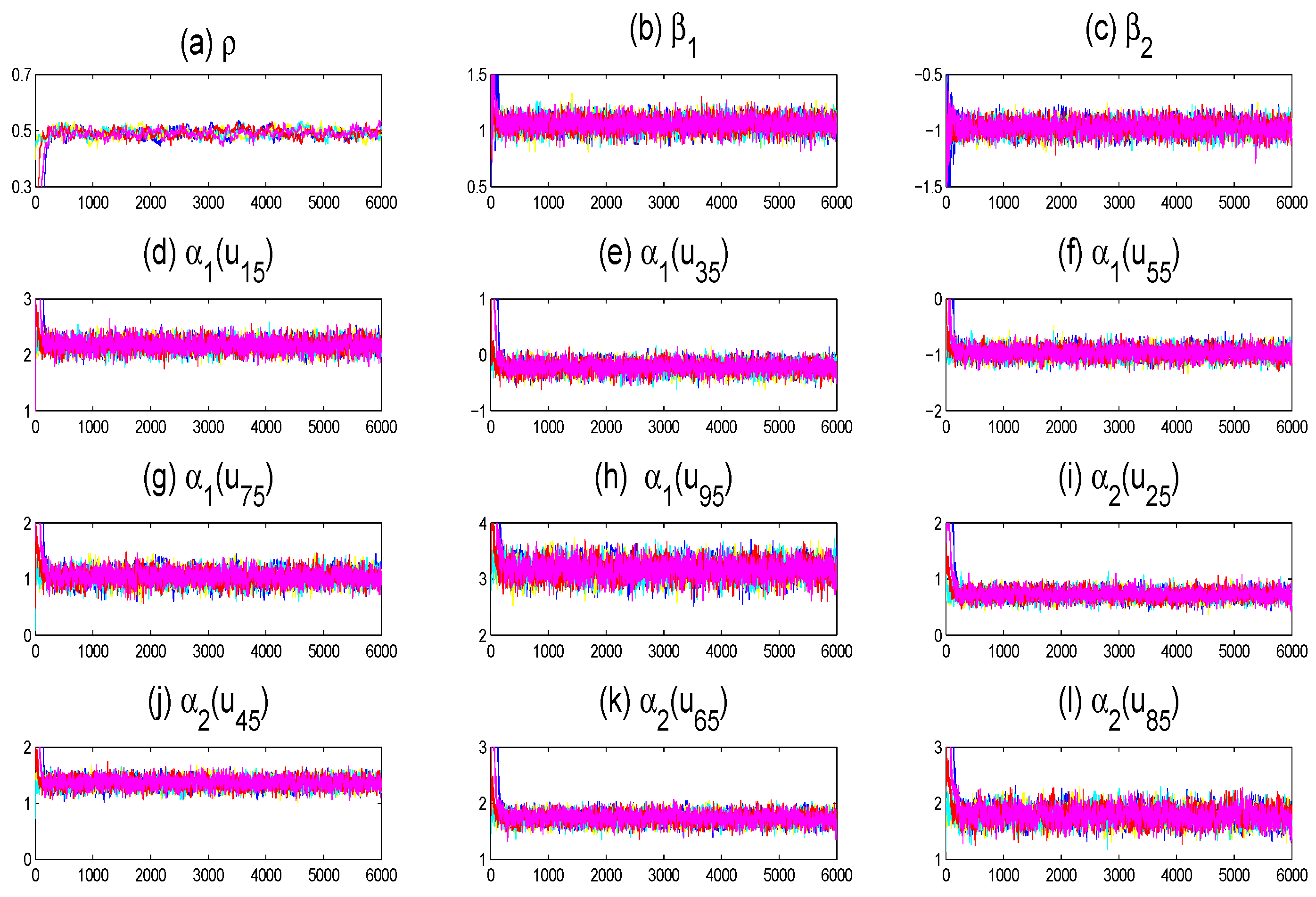
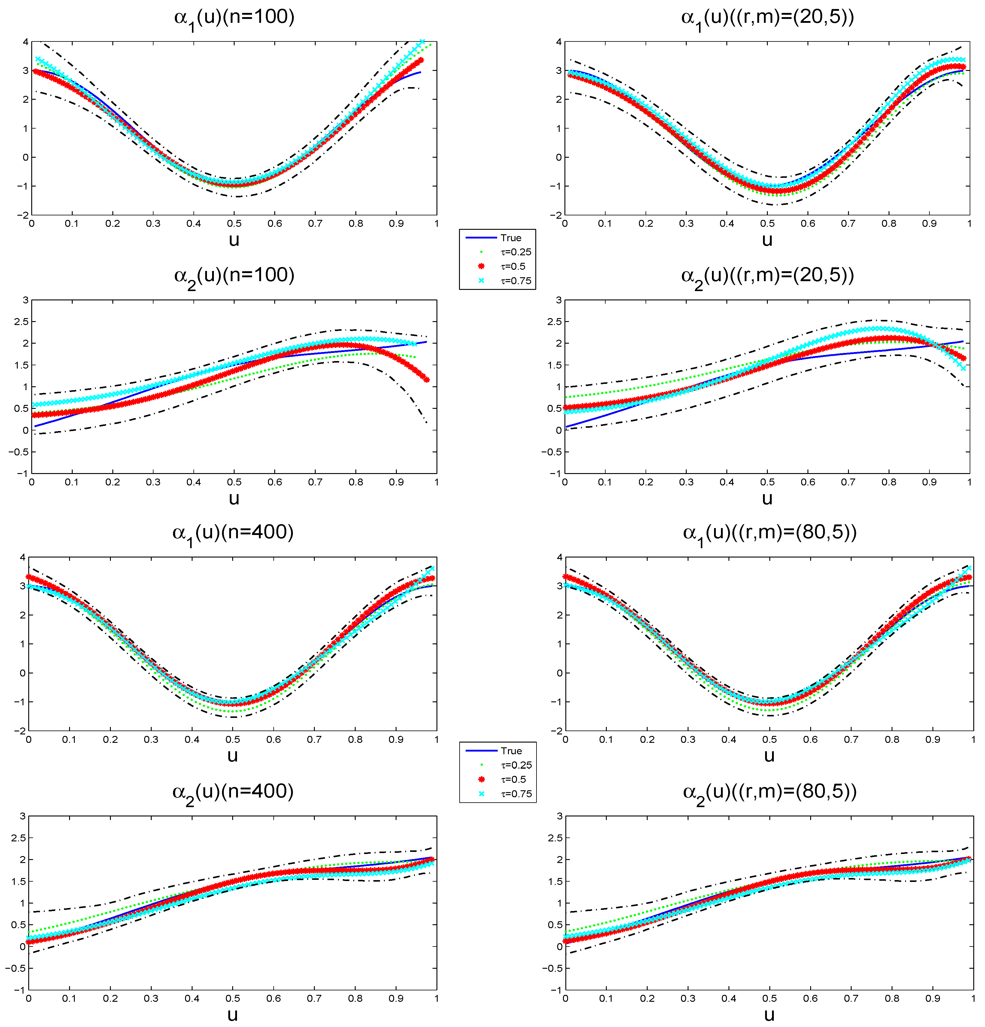
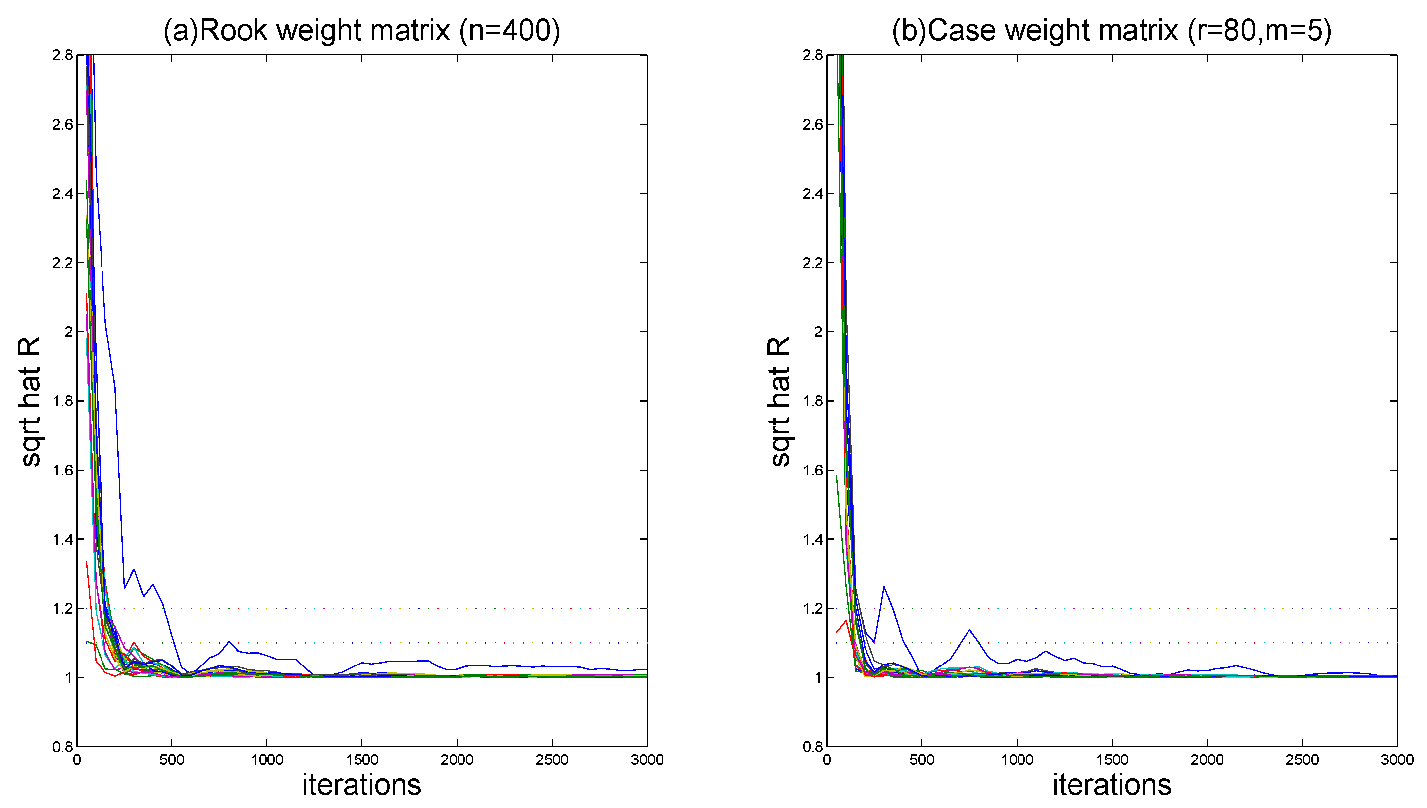
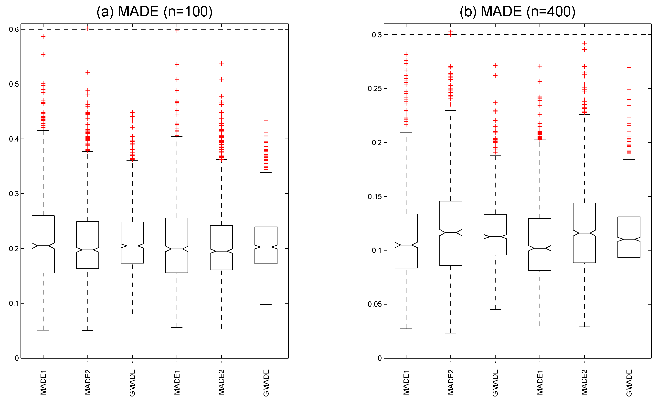
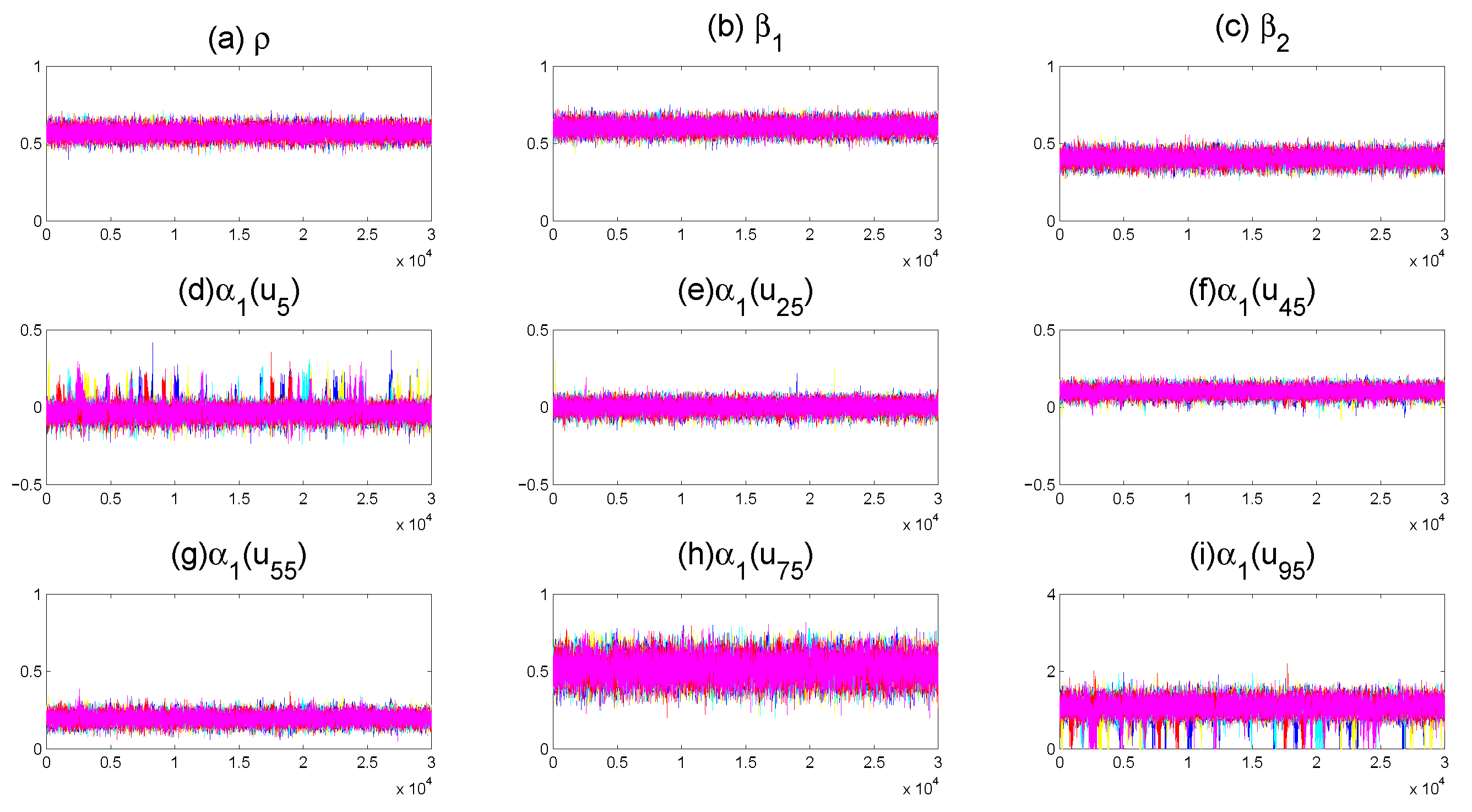
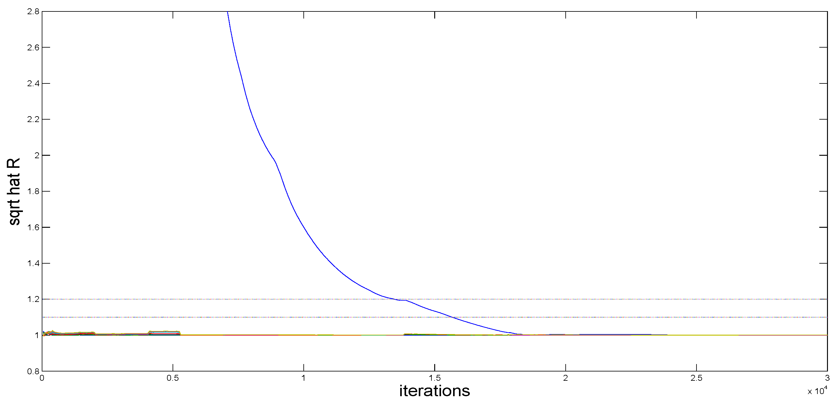
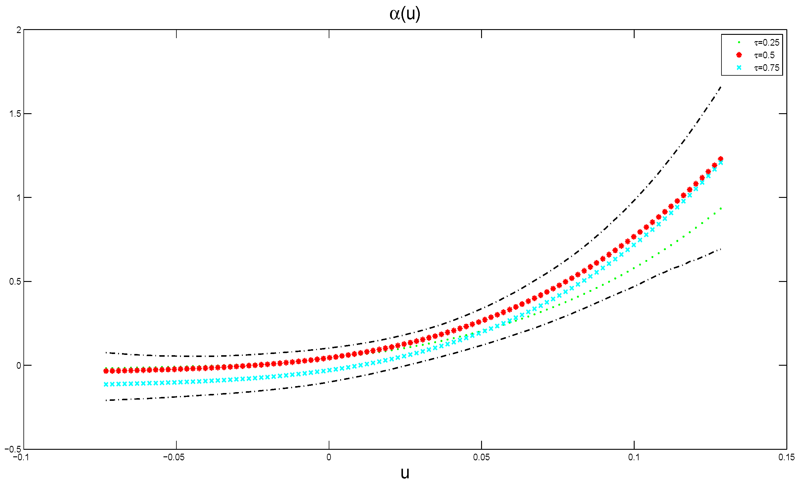
4.1. Simulation

The samples are generated from the following model:

$$y_i=\rho \sum _{j=1}^n{w}_{ij}{y}_j+x_i^{\top }\beta +z_i^{\top }\alpha \left(u_i\right)+{\epsilon }_i,i=1,\cdots ,n,$$

(19)

where the covariate vectors $x_i={(x_{i1},x_{i2})}^{\top }$ follows a bivariate normal distribution with mean vector $\mathbf{0}$ and covariance matrix

$$\Sigma =\left(\begin{array}{cc}1& -0.5\\ -0.5& 1\end{array}\right).$$

$z_i={(z_{i1},z_{i2})}^{\top }$ and $u_i={(u_{i1},u_{i2})}^T$ are bivariate, $z_{ij}\sim \mathrm{U}(-2,0)$ and $u_{ij}\sim \mathrm{U}(0,1)$ for $j=1,2$, $\beta ={(1,-1)}^{\top }$ and the error term ${\epsilon }_i={ϵ}_i-F^{-1}\left(\tau \right)$, where F is the common cumulative distribution function of ${ϵ}_i\sim N(0,1)$. By subtracting the $\tau$th quantile, the error term is equal to zero at the $\tau$th quantile. The varying coefficient functions $\alpha \left(u\right)={({\alpha }_1\left(u_1\right),{\alpha }_2\left(u_2\right))}^{\top }$ with ${\alpha }_1\left(u_1\right)=2cos\left(2\pi u_1\right)+1$ and ${\alpha }_2\left(u_2\right)=0.5exp\{-2{(2u_2-1)}^2\}+2u_2$. Furthermore, we chose three different values of spatial parameters $\rho =\{0.2,0.5,0.8\}$ at three different quantile points $\tau =\{0.25,0.5,0.75\}$, two kinds of the Rook and Case weight matrix as the spatial weight matrix W, respectively. The sample sizes are $n=\{100,400\}$ for the Rook weight matrix, districts and members are $(r,m)=\left\{\right(20,5),(80,5\left)\right\}$ for the Case weight matrix.

We conducted each simulation with 1000 replications. For $j=1,\cdots ,p$, we use a quadratic P-splines in which the number of knots $K_j=18$ are placed at equally spaced interval of the predictor variables and design hyper-parameters $(r_0,s_0^2,r_{{\tau }_0},s_{{\tau }_0}^2,r_{{\tau }_{j0}},s_{{\tau }_{j0}}^2)=(1,1,1,0.005,1,0.005)$ in our computation. The second-order random walk penalties are used for the Bayesian P-splines to approximate the unknown smooth functions. The unknown parameters are drawn from their respective prior distributions. The tuning parameter ${\sigma }_{\rho }$ is used to control the resultant acceptable rate for parameter around 25% by incrementally increasing or decreasing value.

We generated 6000 sampled values following the proposed Gibbs sampler and deleted the first 3000 values as a burn-in period for each of the replications until the Markov Chains reach steady state. According to the last 3000 values, we calculate the corresponding means across 1000 replications for the posterior mean (Mean), standard error (SE) and 2.5th and 97.5th percentiles of the parameters, namely the 95% posterior credible intervals (95% CI), which are defined by the posterior probability of the parameters falling into the intervals is 95% based on the highest posterior density.

We also computed the standard derivations (SD) of the estimated posterior means to compare them with the means of the estimated posterior SE. From the model (19), LeSage and Pace [60] suggested scalar summary measures for the marginal effects, which are given by $\frac{\partial y}{\partial x_j}={(I_n-\rho W)}^{-1}{I}_n{\beta }_j$ for $j=1,\cdots ,q$. The direct effects are labeled as the average of the diagonal elements. The average of either the row sums or the column sums of the non-diagonal elements are used as the indirect effects, and the total effects are the sum of the direct and indirect effects.

To check the convergence of the MCMC algorithm, five different Markov Chains corresponding to different starting values have been ran through the Gibbs sampler to perform each replication. Figure 1 displays the sampled traces of parts of the unknown quantities, including model parameters and fitting functions on grid points. It is clear that the five parallel sequences mix reasonably well. We further calculate the “potential scale reduction factor” $\sqrt{\widehat{R}}$ for all unknown parameters and varying coefficient functions on 10 selected grid points based on the five parallel sequences. Figure 2 shows the values of $\sqrt{\widehat{R}}$ after iterating 3000 times. We observe that all the values of $\sqrt{\widehat{R}}$ are less than 1.2 following the suggestion of Gelman and Rubin [61] after 3000 burn-in iterations, which is sufficient for convergence.

In order to investigate the finite sample performance of varying coefficient functions, the variability measures of the mean absolute deviation errors (MADE) and global mean absolute deviation errors (GMADE) are used to measure the estimation performance. MADE and GMADE are defined as

$${\mathrm{MADE}}_j|{\widehat{\alpha }}_j(·)|=\frac{1}{100}\sum _{i=1}^{100}|{\widehat{\alpha }}_j\left(u_{ij}\right)-{\alpha }_j\left(u_{ij}\right)\left|\mathrm{and}\mathrm{GMADE}\right|\widehat{\alpha }(·)|=\frac{1}{p}\sum _{j=1}^p{\mathrm{MADE}}_j\left|{\widehat{\alpha }}_j(·)\right|$$

at 100 fixed grid points ${\left\{u_{ij}\right\}}_{i=1}^{100}$ that are equally-spaced chosen from interval $[a_j,b_j]$. Figure 3a displays the boxplots of the MADE and GMADE values with sample size $n=100$ and $\rho =0.5$ at $\tau =0.5$ quantile point. Based on the Rook weight matrix on the left three panels, the medians are ${\mathrm{MADE}}_1=0.2049$, ${\mathrm{MADE}}_2=0.1976$ and $\mathrm{GMADE}=0.2048$. Based on the Case weight matrix on the right three panels, the medians are ${\mathrm{MADE}}_1=0.1993$, ${\mathrm{MADE}}_2=0.1952$ and $\mathrm{GMADE}=0.2028$. Figure 3b shows the boxplots of the MADE and GMADE values with sample size $n=400$ and $\rho =0.5$ at $\tau =0.5$ quantile point. Based on the Rook weight matrix, the medians are ${\mathrm{MADE}}_1=0.1049$, ${\mathrm{MADE}}_2=0.1164$ and $\mathrm{GMADE}=0.1126$ on the left three boxplots. Based on the Case weight matrix , the medians are ${\mathrm{MADE}}_1=0.1019$, ${\mathrm{MADE}}_2=0.1160$ and $\mathrm{GMADE}=0.1101$ on the right three boxplots. We can see that the MADE and GMADE values not only decrease when the number of n increase but also become smaller under the Case weight matrix than the Rook weight matrix, meaning the varying coefficient functions become more accurate when increasing the sample size with application of the Case weight matrix. This shows that the proposed model and estimation method with both the Rook weight matrix and the Case weight matrix in the finite sample can obtain reasonable estimation and good performance.

Table 1. Simulation results of the parameter estimation for $\tau =\{0.25,0.5,0.75\}$.

$\mathit{\tau }$	Para.	n	Rook Weight Matrix				$(\mathit{r},\mathit{m})$	Case Weight Matrix
			Mean	SE	SD	95% CI		Mean	SE	SD	95% CI
$0.25$	$\rho =0.2000$	100	$0.1904$	$0.0623$	$0.0706$	$(0.0690,0.3127)$	(20,5)	$0.1895$	$0.05834$	$0.0662$	$(0.0749,0.3037)$
	${\beta }_1=1.0000$		$0.9936$	$0.1242$	$0.1440$	$(0.7493,1.2367)$		$0.9916$	$0.1244$	$0.1435$	$(0.7479,1.2354)$
	${\beta }_2=-1.0000$		$-0.9923$	$0.1241$	$0.1483$	$(-1.2359,-0.7488)$		$-0.9930$	$0.1244$	$0.1487$	$(-1.2367,-0.7490)$
	Total effect
	$x_1=1.2500$		$1.2432$	$0.1838$	$0.2049$	$(0.9039,1.6259)$		$1.2372$	$0.1795$	$0.2010$	$(0.9040,1.6079)$
	$x_2=-1.2500$		$-1.2424$	$0.1832$	$0.2159$	$(-1.6241,-0.9048)$		$-1.2402$	$0.1799$	$0.2138$	$(-1.6119,-0.9054)$
	$\rho =0.5000$		$0.4879$	$0.0496$	$0.0566$	$(0.3900,0.5840)$		$0.4904$	$0.0394$	$0.0459$	$(0.4123,0.5671)$
	${\beta }_1=1.0000$		$0.9944$	$0.1249$	$0.1443$	$(0.7496,1.2383)$		$0.9937$	$0.1246$	$0.1447$	$(0.7496,1.2380)$
	${\beta }_2=-1.0000$		$-0.9942$	$0.1248$	$0.1479$	$(-1.2391,-0.7506)$		$-0.9940$	$0.1243$	$0.1483$	$(-1.2381,-0.7502)$
	Total effect
	$x_1=2.0000$		$1.9818$	$0.3141$	$0.3487$	$(1.4170,2.6498)$		$1.9744$	$0.2863$	$0.3237$	$(1.4430,2.5666)$
	$x_2=-2.0000$		$-1.9830$	$0.3126$	$0.3653$	$(-2.6487,-1.4217)$		$-1.9774$	$0.2868$	$0.3420$	$(-2.5704,-1.4446)$
	$\rho =0.8000$		$0.7909$	$0.0234$	$0.0270$	$(0.7447,0.8365)$		$0.7949$	$0.0168$	$0.0200$	$(0.7613,0.8273)$
	${\beta }_1=1.0000$		$0.9914$	$0.1242$	$0.1429$	$(0.7477,1.2348)$		$0.9957$	$0.1254$	$0.1456$	$(0.7499,1.2415)$
	${\beta }_2=-1.0000$		$-0.9938$	$0.1243$	$0.1447$	$(-1.2381,-0.7505)$		$-0.9964$	$0.1251$	$0.1491$	$(-1.2422,-0.7514)$
	Total effect
	$x_1=5.0000$		$4.8700$	$0.8256$	$0.8677$	$(3.4306,6.6730)$		$4.9200$	$0.7107$	$0.8079$	$(3.5967,6.3884)$
	$x_2=-5.0000$		$-4.8891$	$0.8199$	$0.9282$	$(-6.6744,-3.4559)$		$-4.9292$	$0.7128$	$0.8545$	$(-6.4029,-3.6029)$
$0.50$	$\rho =0.2000$	100	$0.1926$	$0.0585$	$0.0616$	$(0.0771,0.3063)$	(20,5)	$0.1913$	$0.0553$	$0.0581$	$(0.0819,0.2987)$
	${\beta }_1=1.0000$		$0.9926$	$0.1255$	$0.1299$	$(0.7456,1.2381)$		$0.9920$	$0.1254$	$0.1303$	$(0.7455,1.2372)$
	${\beta }_2=-1.0000$		$-0.9951$	$0.1249$	$0.1356$	$(-1.2401,-0.7499)$		$-0.9958$	$0.1248$	$0.1335$	$(-1.2403,-0.7507)$
	Total effect
	$x_1=1.2500$		$1.2426$	$0.1808$	$0.1852$	$(0.9051,1.6148)$		$1.2377$	$0.1776$	$0.1784$	$(0.9044,1.6013)$
	$x_2=-1.2500$		$-1.2466$	$0.1814$	$0.1978$	$(-1.6211,-0.9089)$		$-1.2438$	$0.1773$	$0.1912$	$(-1.6072,-0.9110)$
	$\rho =0.5000$		$0.4924$	$0.0444$	$0.0481$	$(0.4042,0.5783)$		$0.4933$	$0.0369$	$0.0392$	$(0.4194,0.5646)$
	${\beta }_1=1.0000$		$0.9921$	$0.1257$	$0.1300$	$(0.7449,1.2383)$		$0.9918$	$0.1254$	$0.1309$	$(0.7453,1.2373)$
	${\beta }_2=-1.0000$		$-0.9986$	$0.1250$	$0.1357$	$(-1.2439,-0.7536)$		$-0.9994$	$0.1249$	$0.1350$	$(-1.2443,-0.7547)$
	Total effect
	$x_1=2.0000$		$1.9850$	$0.3017$	$0.3097$	$(1.4309,2.6166)$		$1.9765$	$0.2834$	$0.2873$	$(1.4433,2.5567)$
	$x_2=-2.0000$		$-1.9994$	$0.3032$	$0.3310$	$(-2.6347,-1.4442)$		$-1.9935$	$0.2829$	$0.3083$	$(-2.5729,-1.4631)$
	$\rho =0.8000$		$0.7965$	$0.0197$	$0.0218$	$(0.7577,0.8346)$		$0.7967$	$0.0158$	$0.0172$	$(0.7649,0.8270)$
	${\beta }_1=1.0000$		$0.9938$	$0.1260$	$0.1300$	$(0.7466,1.2409)$		$0.9934$	$0.1262$	$0.1307$	$(0.7456,1.2411)$
	${\beta }_2=-1.0000$		$-1.0015$	$0.1258$	$0.1320$	$(-1.2483,-0.7548)$		$-0.9978$	$0.1256$	$0.1368$	$(-1.2444,-0.7516)$
	Total effect
	$x_1=5.0000$		$4.9793$	$0.7911$	$0.8004$	$(3.5531,6.6600)$		$4.9397$	$0.7075$	$0.7209$	$(3.6094,6.3893)$
	$x_2=-5.0000$		$-5.0202$	$0.7887$	$0.8355$	$(-6.6920,-3.5937)$		$-4.9663$	$0.7078$	$0.7807$	$(-6.4156,-3.6369)$
$0.75$	$\rho =0.2000$	100	$0.1944$	$0.0526$	$0.0585$	$(0.0894,0.2962)$	(20,5)	$0.1942$	$0.0507$	$0.0582$	$(0.0927,0.2917)$
	${\beta }_1=1.0000$		$0.9916$	$0.1254$	$0.1454$	$(0.7459,1.2379)$		$0.9927$	$0.1250$	$0.1440$	$(0.7475,1.2384)$
	${\beta }_2=-1.0000$		$-0.9944$	$0.1258$	$0.1482$	$(-1.2411,-0.7482)$		$-0.9941$	$0.1255$	$0.1477$	$(-1.2403,-0.7483)$
	Total effect
	$x_1=1.2500$		$1.2424$	$0.1765$	$0.2007$	$(0.9092,1.6014)$		$1.2430$	$0.1744$	$0.1993$	$(0.9122,1.5965)$
	$x_2=-1.2500$		$-1.2466$	$0.1771$	$0.2089$	$(-1.6063,-0.9118)$		$-1.2444$	$0.1749$	$0.2019$	$(-1.5978,-0.9120)$
	$\rho =0.5000$		$0.4945$	$0.0384$	$0.0456$	$(0.4179,0.5677)$		$0.4945$	$0.0338$	$0.0402$	$(0.4266,0.5591)$
	${\beta }_1=1.0000$		$0.9925$	$0.1256$	$0.1467$	$(0.7463,1.2393)$		$0.9935$	$0.1257$	$0.1437$	$(0.7475,1.2408)$
	${\beta }_2=-1.0000$		$-0.9951$	$0.1258$	$0.1487$	$(-1.2421,-0.7481)$		$-0.9947$	$0.1259$	$0.1483$	$(-1.2420,-0.7485)$
	Total effect
	$x_1=2.0000$		$1.9891$	$0.2897$	$0.3337$	$(1.4451,2.5824)$		$1.9845$	$0.2787$	$0.3161$	$(1.4561,2.5499)$
	$x_2=-2.0000$		$-1.9961$	$0.2908$	$0.3511$	$(-2.5915,-1.4499)$		$-1.9868$	$0.2791$	$0.3238$	$(-2.5521,-1.4570)$
	$\rho =0.8000$		$0.7971$	$0.0160$	$0.0191$	$(0.7651,0.8275)$		$0.7970$	$0.0144$	$0.0171$	$(0.7679,0.8242)$
	${\beta }_1=1.0000$		$0.9936$	$0.1258$	$0.1465$	$(0.7471,1.2407)$		$0.9946$	$0.1259$	$0.1446$	$(0.7488,1.2428)$
	${\beta }_2=-1.0000$		$-0.9955$	$0.1259$	$0.1488$	$(-1.2430,-0.7490)$		$-0.9961$	$0.1263$	$0.1491$	$(-1.2443,-0.7489)$
	Total effect
	$x_1=5.0000$		$4.9663$	$0.7327$	$0.8417$	$(3.5982,6.4729)$		$4.9498$	$0.6930$	$0.8105$	$(3.6354,6.3539)$
	$x_2=-5.0000$		$-4.9777$	$0.7341$	$0.8725$	$(-6.4838,-3.606)$		$-4.9575$	$0.6969$	$0.0939$	$(-6.3666,-3.6328)$

and

Table 2. Simulation results of the parameter estimation for $\tau =\{0.25,0.5,0.75\}$.

$\mathit{\tau }$	Para.	n	Rook Weight Matrix				$(\mathit{r},\mathit{m})$	Case Weight Matrix
			Mean	SE	SD	95% CI		Mean	SE	SD	95% CI
$0.25$	$\rho =0.2000$	400	$0.1958$	$0.0292$	$0.0375$	$(0.1386,0.2533)$	(80,5)	$0.1960$	$0.0267$	$0.0338$	$(0.1438,0.2485)$
	${\beta }_1=1.0000$		$0.9976$	$0.0589$	$0.0724$	$(0.8822,1.1126)$		$0.9983$	$0.0588$	$0.0724$	$(0.8834,1.1133)$
	${\beta }_2=-1.0000$		$-0.9973$	$0.0587$	$0.0721$	$(-1.1122,-0.8824)$		$-0.9975$	$0.0587$	$0.0720$	$(-1.1123,-0.8825)$
	Total effect
	$x_1=1.2500$		$1.2449$	$0.0856$	$0.1089$	$(1.0818,1.4173)$		$1.2451$	$0.0836$	$0.1037$	$(1.0854,1.4127)$
	$x_2=-1.2500$		$-1.2443$	$0.0859$	$0.1049$	$(-1.4173,-1.0812)$		$-1.2442$	$0.0837$	$0.1042$	$(-1.4117,-1.0843)$
	$\rho =0.5000$		$0.4956$	$0.0231$	$0.0299$	$(0.4506,0.5408)$		$0.4979$	$0.0180$	$0.0226$	$(0.4616,0.5323)$
	${\beta }_1=1.0000$		$0.9977$	$0.0590$	$0.0729$	$(0.8822,1.1132)$		$0.9979$	$0.0591$	$0.0726$	$(0.8823,1.1135)$
	${\beta }_2=-1.0000$		$-0.9988$	$0.0590$	$0.0716$	$(-1.1138,-0.8837)$		$-0.9983$	$0.0589$	$0.0719$	$(-1.1134,-0.8830)$
	Total effect
	$x_1=2.0000$		$1.9886$	$0.1450$	$0.1852$	$(1.7155,2.2836)$		$1.9900$	$0.1339$	$0.1668$	$(1.7342,2.2582)$
	$x_2=-2.0000$		$-1.9906$	$0.1459$	$0.1784$	$(-2.2877,-1.7161)$		$-1.9909$	$0.1341$	$0.1659$	$(-2.2594,-1.7345)$
	$\rho =0.8000$		$0.7979$	$0.0114$	$0.0152$	$(0.7755,0.8201)$		$0.7985$	$0.0077$	$0.0097$	$(0.7832,0.8135)$
	${\beta }_1=1.0000$		$0.9986$	$0.0590$	$0.0731$	$(0.8833,1.1140)$		$0.9985$	$0.0593$	$0.0734$	$(0.8826,1.1146)$
	${\beta }_2=-1.0000$		$-0.9983$	$0.0587$	$0.0719$	$(-1.1131,-0.8831)$		$-0.9987$	$0.0591$	$0.0726$	$(-1.1145,-0.8831)$
	Total effect
	$x_1=5.0000$		$4.9827$	$0.3979$	$0.5163$	$(4.2478,5.8062)$		$4.9727$	$0.3347$	$0.4163$	$(4.3318,5.6428)$
	$x_2=-5.0000$		$-4.9795$	$0.3988$	$0.4860$	$(-5.8032,-4.2419)$		$-4.9737$	$0.3343$	$0.4173$	$(-5.6435,-4.3342)$
$0.50$	$\rho =0.2000$	400	$0.1958$	$0.0272$	$0.0321$	$(0.1421,0.2486)$	(80,5)	$0.1966$	$0.0250$	$0.0299$	$(0.1475,0.2455)$
	${\beta }_1=1.0000$		$0.9982$	$0.0652$	$0.0754$	$(0.8743,1.1215)$		$0.9995$	$0.0587$	$0.0687$	$(0.8845,1.1146)$
	${\beta }_2=-1.0000$		$-0.9955$	$0.0645$	$0.0744$	$(-1.1185,-0.8718)$		$-0.9958$	$0.0583$	$0.0656$	$(-1.1102,-0.8817)$
	Total effect
	$x_1=1.2500$		$1.2447$	$0.0903$	$0.1051$	$(1.0750,1.4211)$		$1.2424$	$0.0818$	$0.0957$	$(1.0888,1.4113)$
	$x_2=-1.2500$		$-1.2415$	$0.0894$	$0.1044$	$(-1.4170,-1.0729)$		$-1.2424$	$0.0818$	$0.0937$	$(-1.4059,-1.0856)$
	$\rho =0.5000$		$0.4961$	$0.0207$	$0.0290$	$(0.4553,0.5364)$		$0.4974$	$0.0168$	$0.0200$	$(0.4644,0.5300)$
	${\beta }_1=1.0000$		$0.9979$	$0.0652$	$0.0756$	$(0.8741,1.1211)$		$1.0005$	$0.0589$	$0.0685$	$(0.8853,1.1156)$
	${\beta }_2=-1.0000$		$-0.9964$	$0.0645$	$0.0741$	$(-1.1196,-0.8730)$		$-0.9956$	$0.0585$	$0.0654$	$(-1.1104,-0.8811)$
	Total effect
	$x_1=2.0000$		$1.9900$	$0.1463$	$0.1755$	$(1.7149,2.2798)$		$1.9954$	$0.1312$	$0.1529$	$(1.7427,2.2586)$
	$x_2=-2.0000$		$-1.9670$	$0.1451$	$0.1711$	$(-2.2763,-1.7140)$		$-1.9859$	$0.1312$	$0.1496$	$(-2.2482,-1.7344)$
	$\rho =0.8000$		$0.7979$	$0.0096$	$0.0283$	$(0.7790,0.8164)$		$0.7988$	$0.0072$	$0.0085$	$(0.7847,0.8127)$
	${\beta }_1=1.0000$		$0.9978$	$0.0657$	$0.0752$	$(0.8742,1.1215)$		$1.0001$	$0.0592$	$0.0683$	$(0.8844,1.1158)$
	${\beta }_2=-1.0000$		$-0.9982$	$0.0651$	$0.0737$	$(-1.1205,-0.8745)$		$-0.9966$	$0.0588$	$0.0654$	$(-1.1118,-0.8820)$
	Total effect
	$x_1=5.0000$		$4.9841$	$0.3766$	$0.4580$	$(4.2792,5.7414)$		$4.9836$	$0.3296$	$0.3799$	$(4.3511,5.6389)$
	$x_2=-5.0000$		$-4.9863$	$0.3727$	$0.4499$	$(-5.7377,-4.2875)$		$-4.9663$	$0.3277$	$0.3710$	$(-5.6204,-4.3385)$
$0.75$	$\rho =0.2000$	400	$0.1987$	$0.0243$	$0.0317$	$(0.1508,0.2457)$	(80,5)	$0.1971$	$0.0230$	$0.0299$	$(0.1518,0.2418)$
	${\beta }_1=1.0000$		$1.0000$	$0.0585$	$0.0752$	$(0.8855,1.1146)$		$1.0000$	$0.0587$	$0.0748$	$(0.8849,1.1147)$
	${\beta }_2=-1.0000$		$-0.9970$	$0.0584$	$0.0739$	$(-1.1112,-0.8826)$		$-0.9964$	$0.0584$	$0.0742$	$(-1.1107,-0.8819)$
	Total effect
	$x_1=1.2500$		$1.2511$	$0.0820$	$0.1058$	$(1.0933,1.4142)$		$1.2480$	$0.0810$	$0.1015$	$(1.0915,1.4087)$
	$x_2=-1.2500$		$-1.2474$	$0.0817$	$0.1048$	$(-1.4095,-1.0898)$		$-1.2438$	$0.0807$	$0.1045$	$(-1.4039,-1.0882)$
	$\rho =0.5000$		$0.4985$	$0.0178$	$0.0234$	$(0.4634,0.5327)$		$0.4981$	$0.0155$	$0.0200$	$(0.4677,0.5281)$
	${\beta }_1=1.0000$		$0.9999$	$0.0586$	$0.0740$	$(0.8850,1.1144)$		$0.9997$	$0.0588$	$0.0748$	$(0.8847,1.1146)$
	${\beta }_2=-1.0000$		$-0.9967$	$0.0585$	$0.0740$	$(-1.1114,-0.8823)$		$-0.9971$	$0.0586$	$0.0741$	$(-1.1116,-0.8827)$
	Total effect
	$x_1=2.0000$		$2.0001$	$0.1349$	$0.1729$	$(1.7414,2.2689)$		$1.9961$	$0.1296$	$0.1629$	$(1.7460,2.2533)$
	$x_2=-2.0000$		$-1.9941$	$0.1343$	$0.1729$	$(-2.2622,-1.7365)$		$-1.9913$	$0.1294$	$0.1662$	$(-2.2480,-1.7418)$
	$\rho =0.8000$		$0.7993$	$0.0078$	$0.0107$	$(0.7838,0.8144)$		$0.7990$	$0.0066$	$0.0086$	$(0.7859,0.8116)$
	${\beta }_1=1.0000$		$1.0001$	$0.0587$	$0.0750$	$(0.8853,1.1150)$		$1.0007$	$0.0589$	$0.0753$	$(0.8855,1.1161)$
	${\beta }_2=-1.0000$		$-0.9964$	$0.0585$	$0.0738$	$(-1.1111,-0.8821)$		$-0.9970$	$0.0587$	$0.0745$	$(-1.1120,-0.8824)$
	Total effect
	$x_1=5.0000$		$5.0040$	$0.3456$	$0.4462$	$(4.3430,5.6963)$		$4.9901$	$0.3233$	$0.4063$	$(4.3664,5.6310)$
	$x_2=-5.0000$		$-4.9868$	$0.3451$	$0.4524$	$(-5.6767,-4.3267)$		$-4.9730$	$0.3220$	$0.4205$	$(-5.6121,-4.3508)$

summarize the estimation results. The parameter estimates are quite different at three quantiles of the response distributions. Under the same spatial weight matrix, the accuracy of the results improves with the increasing of the sample sizes. We can see that the means of the unknown estimators are close to the respective true values, and the average values of the SE are close to the corresponding SD, indicating that the parameter estimates and the standard errors are more precise. For the parameter $\rho$ under the same sample sizes, we find the SE and SD of parameter $\rho$ with the Case weight matrix are slightly better than that with the Rook weight matrix. In addition, the general pattern from the estimates reported in Table 1 and Table 2 is that all estimators impose relatively larger bias on the total effect estimates when there is strong positive spatial dependence for similar sample sizes. When we repeat the aforementioned experiences with different starting values, the estimation results are similar, all of which indicate that the proposed Gibbs sampler performs quite well.

Figure 4 compares the estimation results of varying coefficient functions at different quantiles, along with its 95% pointwise posterior credible intervals of ${\alpha }_1\left(u\right)$ and ${\alpha }_2\left(u\right)$ from a typical sample under $(\rho ,n)=(0.5,100)$ and $(\rho ,n)=(0.5,400)$, respectively. The typical sample is selected in such a way that its MADE value is equal to the median in the 1000 replications. We can see that the three fitting curves are fairly close to the solid curve, and the corresponding credible bandwidth is narrow. With the increasing of the sample sizes, the gaps between the fitting curves and the true value become short. There also exist visible differences at different quantiles of the response distributions. It illustrates that the varying coefficient function estimation procedure works well for small samples.

We compare the performance of the Bayesian quantile regression (BQR) estimator in this paper to the instrumental variable quantile regression (IVQR) estimator in Dai et al. [12] with two examples.

Example 1.

The model is given as follows

$$y_i=\rho \sum _{j=1}^n{w}_{ij}{y}_j+x_i\beta +z_{i1}{\alpha }_1\left(u_i\right)+z_{i2}{\alpha }_2\left(u_i\right)+{\epsilon }_i,i=1,\cdots ,n.$$

where $\rho =0.5$, $\beta =1$, ${\alpha }_1\left(u\right)=1-0.5u$ and ${\alpha }_2\left(u\right)=1+sin\left(\sqrt{2}\pi u\right)$, ${\epsilon }_i={ϵ}_i-F^{-1}\left(\tau \right)$, F is the common cumulative distribution function of ${ϵ}_i$, and the $\tau$th quantile of random error ${ϵ}_i$ is centred to zero. $x_i$ and $u_i$ are generated from $N[0,1]$ and $\mathrm{U}[0,2]$, $z_i={(z_{i1},z_{i2})}^{\top }$ are bivariate. $z_{i1}$ and $z_{i2}$ are generated independently from $\mathrm{U}[-2,2]$ and $N(1,1)$.

Table 3. Simulation results of the parameter estimation.

n	Para.	$\mathit{\tau }$	QR				IVQR				BQR
			0.25	0.50	0.75		0.25	0.50	0.75		0.25	0.50	0.75
100	$\rho$	Bias	$0.0214$	$0.0373$	$0.0528$		$0.0037$	$0.0025$	$0.0021$		$0.0093$	$0.0115$	$0.0166$
		RMSE	$0.0516$	$0.0700$	$0.0993$		$0.1315$	$0.1186$	$0.1329$		$0.0446$	$0.0533$	$0.0701$
	$\beta$	Bias	$-0.0063$	$-0.0036$	$-0.0149$		$-0.0065$	$-0.0030$	$0.0041$		$0.0020$	$0.0036$	$0.0008$
		RMSE	$0.1440$	$0.1334$	$0.1460$		$0.1431$	$0.1364$	$0.1508$		$0.1309$	$0.1222$	$0.1310$
	${\alpha }_1(·)$	${\mathrm{MADE}}_1$	$0.2203$	$0.1973$	$0.2207$		$0.2202$	$0.2031$	$0.2200$		$0.1829$	$0.1703$	$0.1787$
	${\alpha }_2(·)$	${\mathrm{MADE}}_2$	$0.2038$	$0.1930$	$0.2002$		$0.2139$	$0.1971$	$0.2145$		$0.2030$	$0.1910$	$0.2001$
200	$\rho$	Bias	$0.0198$	$0.0341$	$0.0569$		$0.0016$	$0.0008$	$-0.0011$		$0.0023$	$0.0035$	$0.0057$
		RMSE	$0.0372$	$0.0527$	$0.0804$		$0.0853$	$0.0761$	$0.0859$		$0.0304$	$0.0355$	$0.0466$
	$\beta$	Bias	$-0.0054$	$-0.0044$	$-0.0171$		$0.0003$	$-0.0016$	$0.0021$		$-0.0014$	$-0.0009$	$-0.0024$
		RMSE	$0.1010$	$0.0930$	$0.1035$		$0.1009$	$0.0918$	$0.0966$		$0.0912$	$0.0840$	$0.0891$
	${\alpha }_1(·)$	${\mathrm{MADE}}_1$	$0.1479$	$0.1379$	$0.1491$		$0.1520$	$0.1377$	$0.1515$		$0.1328$	$0.1250$	$0.1317$
	${\alpha }_2(·)$	${\mathrm{MADE}}_2$	$0.1533$	$0.1425$	$0.1452$		$0.1513$	$0.1423$	$0.1530$		$0.1480$	$0.1392$	$0.1445$
500	$\rho$	Bias	$0.0213$	$0.0384$	$0.0572$		$0.0025$	$-0.0006$	$0.0009$		$0.0013$	$0.0009$	$0.0009$
		RMSE	$0.0297$	$0.0463$	$0.0672$		$0.0539$	$0.0462$	$0.0520$		$0.0194$	$0.0229$	$0.0292$
	$\beta$	Bias	$-0.008$	$-0.0103$	$-0.0106$		$-0.0011$	$-0.0002$	$-0.0010$		$0.0020$	$0.0019$	$0.0006$
		RMSE	$0.0600$	$0.0590$	$0.0635$		$0.0599$	$0.0600$	$0.0635$		$0.0587$	$0.0520$	$0.0598$
	${\alpha }_1(·)$	${\mathrm{MADE}}_1$	$0.0925$	$0.0862$	$0.0921$		$0.0919$	$0.0857$	$0.0914$		$0.0882$	$0.0824$	$0.0875$
	${\alpha }_2(·)$	${\mathrm{MADE}}_2$	$0.1066$	$0.1083$	$0.1044$		$0.1040$	$0.1027$	$0.1041$		$0.0918$	$0.0833$	$0.0877$
800	$\rho$	Bias	$0.0226$	$0.0362$	$0.0599$		$-0.0002$	$-0.0006$	$-0.0004$		$0.0009$	$0.0005$	$0.0009$
		RMSE	$0.0280$	$0.0413$	$0.0660$		$0.0405$	$0.0385$	$0.0402$		$0.0154$	$0.0181$	$0.0229$
	$\beta$	Bias	$-0.0038$	$-0.0064$	$-0.0116$		$-0.0029$	$-0.0020$	$0.0005$		$-0.0007$	$0.0009$	$0.0014$
		RMSE	$0.0486$	$0.0451$	$0.0485$		$0.0478$	$0.0443$	$0.0476$		$0.0463$	$0.0427$	$0.0471$
	${\alpha }_1(·)$	${\mathrm{MADE}}_1$	$0.0721$	$0.0675$	$0.0722$		$0.0711$	$0.0674$	$0.0701$		$0.0710$	$0.0669$	$0.0700$
	${\alpha }_2(·)$	${\mathrm{MADE}}_2$	$0.0981$	$0.0956$	$0.0947$		$0.0741$	$0.0892$	$0.0924$		$0.0713$	$0.0658$	$0.0687$

summarizes the comparison results of QR, IVQR and BQR estimators with a homoscedastic error term.

Example 2.

The model is given as follows

$$y_i=\rho \sum _{j=1}^n{w}_{ij}{y}_j+x_i\beta +z_{i1}{\alpha }_1\left(u_i\right)+z_{i2}{\alpha }_2\left(u_i\right)+(1+0.5z_{i1}){\epsilon }_i,i=1,\cdots ,n.$$

where $\rho =0.5$, $\beta =1$, ${\alpha }_1\left(u\right)=1-0.5u$ and ${\alpha }_2\left(u\right)=0.5u^2-u+1$, ${\epsilon }_i={ϵ}_i-F^{-1}\left(\tau \right)$, F is the common cumulative distribution function of ${ϵ}_i$, and the $\tau$th quantile of random error ${ϵ}_i$ is equal to zero. $x_i$ and $u_i$ are generated from $N[0,1]$, and $\mathrm{U}[0,2]$, $z_i={(z_{i1},z_{i2})}^{\top }$ are bivariate. $z_{i1}$ and $z_{i2}$ are generated independently from $N(0,1)$ and $\mathrm{U}[-2,2]$.

Table 4. Simulation results of parameter estimation.

n	Para.	$\mathit{\tau }$	QR				IVQR				BQR
			0.25	0.50	0.75		0.25	0.50	0.75		0.25	0.50	0.75
100	$\rho$	Bias	$0.0477$	$0.0861$	$0.0560$		$0.0070$	$0.0011$	$0.0009$		$0.0208$	$0.0169$	$0.0180$
		RMSE	$0.0835$	$0.1252$	$0.0915$		$0.1289$	$0.1197$	$0.1289$		$0.0657$	$0.0721$	$0.0660$
	$\beta$	Bias	$-0.0147$	$-0.0204$	$-0.0101$		$-0.0074$	$0.0014$	$-0.0026$		$0.0009$	$0.0012$	$-0.0020$
		RMSE	$0.1298$	$0.1222$	$0.1309$		$0.1326$	$0.1155$	$0.1325$		$0.1150$	$0.1104$	$0.1183$
	${\alpha }_1(·)$	${\mathrm{MADE}}_1$	$0.2257$	$0.1892$	$0.2323$		$0.2317$	$0.1989$	$0.2405$		$0.1969$	$0.1700$	$0.2153$
	${\alpha }_2(·)$	${\mathrm{MADE}}_2$	$0.1953$	$0.1782$	$0.1982$		$0.2004$	$0.1775$	$0.2030$		$0.1727$	$0.1638$	$0.1970$
200	$\rho$	Bias	$0.0445$	$0.0874$	$0.0531$		$-0.0004$	$0.0036$	$-0.0007$		$0.0104$	$0.0081$	$0.0087$
		RMSE	$0.0638$	$0.1049$	$0.0723$		$0.0801$	$0.0740$	$0.0907$		$0.0442$	$0.0484$	$0.0438$
	$\beta$	Bias	$-0.0114$	$-0.0177$	$-0.0133$		$0.0029$	$-0.0008$	$-0.0056$		$-0.0048$	$-0.0007$	$-0.0028$
		RMSE	$0.0837$	$0.0786$	$0.0827$		$0.0819$	$0.0736$	$0.0839$		$0.0795$	$0.0703$	$0.0786$
	${\alpha }_1(·)$	${\mathrm{MADE}}_1$	$0.1337$	$0.1093$	$0.1421$		$0.1406$	$0.1139$	$0.1403$		$0.1338$	$0.1034$	$0.1400$
	${\alpha }_2(·)$	${\mathrm{MADE}}_2$	$0.1231$	$0.1141$	$0.1211$		$0.1256$	$0.1117$	$0.1235$		$0.1225$	$0.1114$	$0.1206$
500	$\rho$	Bias	$0.0433$	$0.0804$	$0.0510$		$-0.0013$	$0.0009$	$-0.0001$		$0.0033$	$0.0007$	$0.0015$
		RMSE	$0.0512$	$0.0878$	$0.0585$		$0.0440$	$0.0429$	$0.0517$		$0.0257$	$0.0277$	$0.0269$
	$\beta$	Bias	$-0.0104$	$-0.0140$	$-0.0117$		$0.0008$	$0.0008$	$-0.0001$		$0.0001$	$0.0014$	$0.0009$
		RMSE	$0.0466$	$0.0464$	$0.0473$		$0.0476$	$0.0420$	$0.0484$		$0.0465$	$0.0418$	$0.0469$
	${\alpha }_1(·)$	${\mathrm{MADE}}_1$	$0.0789$	$0.0548$	$0.0906$		$0.0757$	$0.0582$	$0.0766$		$0.0740$	$0.0545$	$0.0761$
	${\alpha }_2(·)$	${\mathrm{MADE}}_2$	$0.0703$	$0.0643$	$0.0691$		$0.0706$	$0.0628$	$0.0715$		$0.0682$	$0.0619$	$0.0678$
800	$\rho$	Bias	$0.0417$	$0.0776$	$0.0495$		$0.0013$	$0.0013$	$0.0000$		$0.0022$	$0.0000$	$0.0006$
		RMSE	$0.0462$	$0.0823$	$0.0545$		$0.0326$	$0.0340$	$0.0380$		$0.0192$	$0.0213$	$0.0211$
	$\beta$	Bias	$-0.0083$	$-0.0174$	$-0.0081$		$-0.0042$	$-0.0009$	$-0.0014$		$0.0001$	$0.0014$	$0.0014$
		RMSE	$0.0367$	$0.0381$	$0.0347$		$0.0358$	$0.0317$	$0.0346$		$0.0352$	$0.0311$	$0.0343$
	${\alpha }_1(·)$	${\mathrm{MADE}}_1$	$0.0657$	$0.0408$	$0.0762$		$0.0582$	$0.0402$	$0.0585$		$0.0554$	$0.0369$	$0.0575$
	${\alpha }_2(·)$	${\mathrm{MADE}}_2$	$0.0522$	$0.0502$	$0.0530$		$0.0521$	$0.0483$	$0.0526$		$0.0499$	$0.0467$	$0.0504$

summarizes the comparison results of QR, IVQR and BQR estimators with a heteroscedastic error term.

The spatial weight matrix $W=\left(w_{ij}\right)$ is generated based on mechanism that $w_{ij}={0.3}^{\left|i-j\right|}$ for $i,j=1,\cdots ,n$, and then standardized transformation is applied to convert the matrix W to have row-sums of unit [12]. After repeating the estimation procedure 1000 times for each case, we calculate the Bias and RMSE between the parameter estimates and true values, the MADE of the estimation accuracy of the varying coefficient functions.

Table 3 and Table 4 report the results of QR, IVQR and BQR corresponding to example 1 and example 2. It can be seen that the influence of explanatory variables on the response is quite different at different quantiles of the response distributions. When the sample sizes enhance, all the bias, RMSE and MADE of the estimators will decrease significantly. Comparing with the three methods QR, IVQR and BQR, the BQR estimator can obtain more robust results in the same condition with less bias, RMSE and MADE. We think that BQR algorithm is superior to QR and IVQR, although the later can also achieve reasonable estimations.

4.2. Application

As an application of the proposed model and methods to a real data example, we use the well-known Sydney real estate data with detailed description in [62]. The data set contains 37,676 properties sold in the Sydney Statistical Division (an official geographical region including Sydney) in the calendar year of 2001, which is available from HRW package in R. We focus on the last week of February only to avoid the temporal issue including 538 properties.

In this application, the house price (Price) is explained by four variables, which are the distance from house to the nearest coastline location in kilometres (DC), distance from house to the nearest main road in kilometres (DR), inflation rate measured as a percentage (IR) and average weekly income (Income). The DC and DR have linear effects on the response Price, while the IR and Income have nonlinear effects on the response Price. Moreover, we make Price and DC logarithmic transformation to avoid the trouble caused by big gaps in the domain. In addition, Income is transformed so that the marginal distribution is approximately $N(0,1)$. Therefore, the following partially linear varying coefficient spatial autoregressive model will be developed:

$$y_i=\rho \sum _{j=1}^n{w}_{ij}{y}_j+x_i^{\top }\beta +z_i\alpha \left(u_i\right)+{\epsilon }_i,i=1,\cdots ,n,$$

(20)

where the response variable $y_i=log\left({\mathrm{Price}}_i\right)$, $x_{i1}=log\left({\mathrm{DC}}_i\right)$, $x_{i2}={\mathrm{DR}}_i$, $z_{i1}={\mathrm{IR}}_i$, $u_i={\mathrm{Income}}_i$. Regarding the choice of the weight matrix, according to the practice in Sun et al. [10], we use the Euclidean distance in terms of any two houses to calculate the spatial weight matrix W. The location is represented with longitude and latitude, denoted as $s_i=(Lo{n}_i,La{t}_i)$. The spatial weight $w_{il}$ is

$$w_{il}=exp\{-\parallel s_i-s_l\parallel \}/\sum _{k\ne i}exp\{-\parallel s_i-s_k\parallel \}.$$

For this dataset, we adopt quadratic P-splines and hyper-parameters $(\lambda ,r_0,s_0^2,r_{{\tau }_{\alpha 0}},s_{{\tau }_{\alpha 0}}^2,r_{{\tau }_{{\beta }_{j}0}},s_{{\tau }_{{\beta }_{j}0}}^2)$ $=(2,1,1,1,0.005,1,0.005)$ for $j=1,\cdots ,p$. The tuning parameter ${\sigma }_{\rho }$ is used to control the acceptable rate for updating $\rho$ around 25%.

We run the proposed Gibbs sampler five times with different starting values and generate 10,000 sampled values following a burn-in of 20,000 iterations in each run. Traces of parts of the unknown quantities are plotted in Figure 5, and the five parallel sequences aggregate very well. Based on the five parallel sequences, we further calculate the “potential scale reduction factor” $\sqrt{\widehat{R}}$, which is plotted in Figure 6. It is clear that all the values of $\sqrt{\widehat{R}}$ are less than 1.2 after 20,000 burn-in iterations. The proposed estimators can realize excellent convergence effects applying to the actual data.

Table 5. Parameter estimation in the model (20) for Sydney real estate data.

$\mathit{\tau }$	$\mathit{\tau }=0.25$				$\mathit{\tau }=0.5$				$\mathit{\tau }=0.75$
Para.	Mean	SE	95%CI		Mean	SE	95%CI		Mean	SE	95%CI
$\rho$	$0.5766$	$0.0077$	$(0.5510,0.5807)$		$0.5700$	$0.0030$	$(0.5657,0.5736)$		$0.5558$	$0.0037$	$(0.5521,0.5640)$
${\beta }_1$	$0.5998$	$0.0291$	$(0.5429,0.6564)$		$0.6039$	$0.0340$	$(0.5373,0.6707)$		$0.6070$	$0.0429$	$(0.5238,0.6913)$
${\beta }_2$	$0.2458$	$0.0239$	$(0.1977,0.2907)$		$0.4033$	$0.0348$	$(0.3321,0.4689)$		$0.8497$	$0.0598$	$(0.7353,0.9667)$
Total effect
$x_1$	$1.4166$	$0.0715$	$(1.2735,1.5597)$		$1.4044$	$0.0763$	$(0.7085,1.5669)$		$1.3665$	$0.0988$	$(1.1690,1.5641)$
$x_2$	$0.5805$	$0.0593$	$(0.4620,0.6992)$		$0.9379$	$0.0783$	$(0.7812,1.0945)$		$1.9128$	$0.1372$	$(1.6384,2.1871)$

lists the estimated parameters together with their standard errors and 95% posterior credible intervals. It shows that the estimation of the spatial coefficient $\widehat{\rho }$ is 0.57 with the standard deviation SE $=0.003$ at $\tau =0.5$ quantile, which means that there exists positive and significant spatial spillover effects for the housing prices of Sydney real estate. However, the spatial coefficient decreases with the increase of quantiles, when the house prices are lower, the spatial effects and the interaction between different regions become stronger. The coefficients of the two covariates $log\left(\mathrm{DC}\right)$ and $\mathrm{DR}$ are ${\widehat{\beta }}_1=0.6039$ and ${\widehat{\beta }}_2=0.4033$ at $\tau =0.5$ quantile, they also have promotional effects on housing prices at the other two quantiles, $log\left(\mathrm{DC}\right)$ and $\mathrm{DR}$ will play an important positive role with the house prices rising because the two parameters present an increasing trend at higher quantiles.

Figure 7 presents the estimated varying coefficient functions together with its 95% pointwise posterior credible intervals, which includes three quantiles $\tau =0.25,\tau =0.5$ and $\tau =0.75$ by a dotted line, star line and forked line, respectively. The curves totally show an upward trend, especially when u becomes larger, the curves rise up more. This shows that the effect of covariate Income on the response has a U-shaped nonlinear relationship. More specifically, when the quantile at $\tau =0.5$, the varying coefficient function $\alpha \left(u\right)$ is greater than the other two, meaning that Income has a significant promoting influence in areas with higher housing prices. The empirical result confirms the robustness and practicability of the Bayesian P-splines method.

5. Summary

This article focused on studying Bayesian estimation and inference in a quantile regression of partially linear varying coefficient spatial autoregressive models with P-splines. This can analyse the linear and nonlinear effects of the covariates on the response for spatial data, reduce the high risk of misspecification of the traditional SAR models and avoid certain serious drawbacks of fully nonparametric models.

We developed Bayesian quantile regression of PLVCSAR models using the asymmetric Laplace error distribution, which can capture comprehensive features at different quantile points without strict restrictions. Moreover, we considered a fully Bayesian P-splines approach to analyse the PLVCSAR models and designed a Gibbs sampler to explore the full conditional posterior distributions. Compared with the QR and IVQR estimators in the same condition, our methodology obtained more robust and precise results. Finally, the proposed model and method with an application were used to analyse a real dataset.

In this article, we considered spatial data with homoscedasticity or heteroscedastic error term, which does not need any specification of error distribution. Although we used a partially linear varying coefficient SAR model, the other models, such as a partially linear single-index SAR model and partially linear additive SAR model can also be considered. In addition, we also need to study variable selection and model selection in a large sample.

References

- Cliff, A.D.; Ord, J.K. Spatial Autocorrelation; Pion Ltd.: London, UK, 1973. [Google Scholar]
- Lee, L.F. Asymptotic Distribution of Quasi-Maximum Likelihood Estimators for Spatial Autoregressive Models. Econometrica 2004, 72, 1899–1925. [Google Scholar] [CrossRef]
- Lee, L.F. GMM and 2SLS Estimation of Mixed Regressive Spatial Autoregressive Models. J. Econom. 2007, 137, 489–514. [Google Scholar] [CrossRef]
- Kakamu, K.; Wago, H. Small-sample properties of panel spatial autoregressive models: Comparison of the Bayesian and maximum likelihood methods. Spat. Econ. Anal. 2008, 3, 305–319. [Google Scholar] [CrossRef]
- Xu, X.B.; Lee, L.F. A spatial autoregressive model with a nonlinear transformation of the dependent variable. J. Econom. 2015, 186, 1–18. [Google Scholar] [CrossRef]
- Basile, R. Regional economic growth in Europe: A semiparametric spatial dependence approach. Pap. Reg. Sci. 2008, 87, 527–544. [Google Scholar] [CrossRef]
- Basile, R. Productivity polarization across regions in Europe: The role of nonlinearities and spatial dependence. Int. Reg. Sci. Rev. 2008, 32, 92–115. [Google Scholar] [CrossRef] [Green Version]
- Basile, R.; Gress, B. Semi-parametric spatial auto-covariance models of regional growth behaviour in Europe. Reg. Dev. 2005, 21, 93–118. [Google Scholar] [CrossRef]
- Paelinck, J.H.P.; Klaassen, L.H. Spatial Econometrics; Gower Press: Aldershot, UK, 1979. [Google Scholar]
- Sun, Y.; Yan, H.J.; Zhang, W.Y.; Lu, Z. A Semiparametric spatial dynamic model. Ann. Stat. 2014, 42, 700–727. [Google Scholar] [CrossRef] [Green Version]
- Chen, J.Q.; Wang, R.F.; Huang, Y.X. Semiparametric spatial autoregressive model: A two-step Bayesian approach. Ann. Public Health Res. 2015, 2, 1012. [Google Scholar]
- Dai, X.; Li, S.; Tian, M. Quantile regression for partially linear varying coefficient spatial autoregressive models. arXiv 2016, arXiv:1608.01739. [Google Scholar]
- Cai, Z.; Xu, X. Nonparametric quantiles estimations for dynamic smooth coefficients models. J. Am. Stat. Assoc. 2008, 103, 1595–1608. [Google Scholar] [CrossRef]
- Bellman, R.E. Adaptive Control Processes; Princeton University Press: Princeton, NJ, USA, 1961. [Google Scholar]
- Hastie, T.J.; Tibshirani, R.J. Generalized Additive Models; Chapman and Hall: New York, NY, USA, 1990. [Google Scholar]
- Friedman, J.H.; Stuetzle, W. Projection Pursuit Regression. J. Am. Stat. Assoc. 1981, 376, 817–823. [Google Scholar] [CrossRef]
- Hastie, T.J.; Tibshirani, R.J. Varying-coefficient models. J. R. Stat. Soc. 1993, 55, 757–796. [Google Scholar] [CrossRef]
- Chiang, C.; Rice, J.; Wu, C. Smoothing Spline Estimation for Varying Coefficient Models with Repeatedly Measured Dependent Variables. J. Am. Stat. Assoc. 2001, 96, 605–619. [Google Scholar] [CrossRef]
- Eubank, R.L.; Huang, C.F.; Buchanan, R.J. Smoothing Spline Estimation in Varying-coefficient Models. J. R. Stat. Soc. 2004, 66, 653–667. [Google Scholar] [CrossRef]
- Lu, Y.Q.; Zhang, R.Q.; Zhu, L.P. Penalized Spline Estimation for Varying-Coefficient Models. Commun. Stat. Theory Methods 2008, 37, 2249–2261. [Google Scholar] [CrossRef]
- Wu, C.O.; Chiang, C.; Hoover, D.R. Asymptotic confidence regions for kernel smoothing of a varying-coefficient model with longitudinal data. J. Am. Stat. Assoc. 1998, 93, 1388–1403. [Google Scholar] [CrossRef]
- Cai, Z.W.; Fan, J.Q.; Li, R.Z. Efficient Estimation and Inferences for Varying Coefficient Models. J. Am. Stat. Assoc. 2000, 451, 888–902. [Google Scholar] [CrossRef]
- Cai, Z.W. Two-Step Likelihood Estimation Procedure for Varying Coefficient Models. J. Multivar. Anal. 2002, 1, 18–209. [Google Scholar] [CrossRef] [Green Version]
- Huang, J.Z.; Wu, C.O.; Zhou, L. Varying-coefficient models and basis functions approximations for the analysis of repeated measurements. Biometrika 2002, 89, 111–128. [Google Scholar] [CrossRef]
- Lu, Y.Q.; Mao, S.S. Local asymptotics for B-spline estimators of the varying-coefficient model. Commun. Stat. 2004, 33, 1119–1138. [Google Scholar] [CrossRef]
- Elhorst, J. Unconditional Maximum Likelihood Estimation of Linear and Log-Linear Dynamic Models for Spatial Panels. Geogr. Anal. 2005, 37, 85–106. [Google Scholar] [CrossRef]
- Yu, J.H.; De Jong, R.; Lee, L.F. Quasi-maximum likelihood estimators for spatial dynamic panel data with fixed effects when both n and t are large. J. Econom. 2008, 146, 118–134. [Google Scholar] [CrossRef] [Green Version]
- Lee, L.F.; Yu, J.H. Estimation of spatial autoregressive panel data models with fixed effects. J. Econom. 2010, 154, 165–185. [Google Scholar] [CrossRef]
- Chen, Z.Y.; Chen, J.B. Bayesian analysis of partially linear additive spatial autoregressive models with free-knot splines. Symmetry 2021, 13, 1635. [Google Scholar] [CrossRef]
- Koenker, R.; Bassett, G. Regression Quantiles. Econometrica 1978, 46, 33–50. [Google Scholar] [CrossRef]
- Jäntschi, L.; Bálint, D.; Bolboacǎ, S.D. Multiple linear regressions by maximizing the likelihood under assumption of generalized Gauss–Laplace distribution of the error. Comput. Math. Methods Med. 2016, 2016, 8578156. [Google Scholar] [CrossRef]
- Koenker, R.; Machado, J. Goodness of Hit and related inference processes for quantile regression. J. Am. Stat. Assoc. 1999, 94, 1296–1309. [Google Scholar] [CrossRef]
- Zerom, G.D. On additive conditional quantiles with high-dimensional covariates. J. Am. Stat. Assoc. 2003, 98, 135–146. [Google Scholar]
- Chernozhukov, V.; Hansen, C. Instrumental variable quantile regression: A robust inference approach. J. Econom. 2008, 142, 379–398. [Google Scholar] [CrossRef] [Green Version]
- Su, L.J.; Yang, Z.L. Instrumental Variable Quantile Estimation of Spatial Autoregressive Models; Working Papers; Singapore Management University: Singapore, 2009. [Google Scholar]
- Koenker, B. Quantile Regression; Cambridge University Press: Cambridge, UK, 2005. [Google Scholar]
- Yu, K.M.; Moyeed, R.A. Bayesian quantile regression. Stat. Probab. Lett. 2001, 54, 437–447. [Google Scholar] [CrossRef]
- Kozubowski, T.J.; Podgórski, K. A multivariate and asymmetric generalization of Laplace distribution. Comput. Stat. 2000, 15, 531–540. [Google Scholar] [CrossRef]
- Yuan, Y.; Yin, G.S. Bayesian quantile regression for longitudinal studies with nonignorable missing data. Biometrics 2010, 66, 105–114. [Google Scholar] [CrossRef]
- Li, Q.; Xi, R.B.; Lin, N. Bayesian regularized quantile regression. Bayesian Anal. 2010, 5, 533–556. [Google Scholar] [CrossRef]
- Lum, K.; Gelfand, A.E. Spatial quantile multiple regression using the asymmetric Laplace process. Bayesian Anal. 2012, 7, 235–258. [Google Scholar] [CrossRef]
- Anselin, L. Spatial Econometrics: Methods and Models; Kluwer Academic Publishers: Dordrecht, The Netherlands, 1988. [Google Scholar]
- Anselin, L. Estimation Methods for Spatial Autoregressive Structures. Reg. Sci. Diss. Monogr. Ser. 1980, 8, 263–273. [Google Scholar]
- Conley, T.G. GMM Estimation with Cross Sectional Dependence. J. Econom. 1999, 92, 1–45. [Google Scholar] [CrossRef]
- LeSage, J. Bayesian Estimation of Spatial Autoregressive Models. Int. Relations 1997, 20, 113–129. [Google Scholar] [CrossRef]
- Dunson, D.B.; Taylor, J.A. Approximate Bayesian inference for quantiles. J. Nonparametr. Stat. 2005, 17, 385–400. [Google Scholar] [CrossRef]
- Thompson, P.; Cai, Y.; Moyeed, R.; Reeve, D.; Stander, J. Bayesian nonparametric quantile regression using splines. Comput. Stat. Data Anal. 1993, 54, 1138–1150. [Google Scholar] [CrossRef]
- Boor, C.D. A Practical Guide to Splines; Springer: New York, NY, USA, 1978. [Google Scholar]
- Krisztin, T. Semi-parametric spatial autoregressive models in freight generation modeling. Transp. Res. Part Logist. Transp. Rev. 2018, 114, 121–143. [Google Scholar] [CrossRef]
- Eilers, P.H.C.; Marx, B.D. Flexible smoothing with B-splines and penalties. Stat. Sci. 1996, 11, 89–121. [Google Scholar] [CrossRef]
- Jäntschi, L. A test detecting the outliers for continuous distributions based on the cumulative distribution function of the data being tested. Symmetry 2019, 11, 835. [Google Scholar] [CrossRef] [Green Version]
- Kozumi, H.; Kobayashi, G. Gibbs sampling methods for bayesian quantile regression. J. Stat. Comput. Simul. 2011, 81, 1565–1578. [Google Scholar] [CrossRef] [Green Version]
- Barndorff-Nielsen, O.E.; Shephard, N. Non-gaussian ornstein-uhlenbeck-based models and some of their uses in financial economics. J. R. Stat. Soc. 2001, 63, 167–241. [Google Scholar] [CrossRef]
- Dagnapur, J.S. An easily implemented generalized inverse Gaussian generator. Commun. Stat. Simul. Comput. 1989, 18, 703–710. [Google Scholar]
- Tierney, L. Markov chains for exploring posterior distributions. Ann. Stat. 1994, 22, 1701–1728. [Google Scholar] [CrossRef]
- Hastings, W.K. Monte Carlo sampling methods using Markov Chains and their applications. Biometrika 1970, 57, 97–109. [Google Scholar] [CrossRef]
- Metropolis, N.; Rosenbluth, A.W.; Rosenbluth, M.N.; Teller, A.H.; Teller, E. Equations of state calculations by fast computing machine. J. Chem. Phys. 1953, 21, 1087–1091. [Google Scholar] [CrossRef] [Green Version]
- Tanner, M.A. Tools for Statistical Inference: Methods for the Exploration of Posterior Distributions and lIkelihood Functions, 2nd ed.; Springer: New York, NY, USA, 1993. [Google Scholar]
- Case, A.C. Spatial patterns in householed demand. Econometrica 1991, 59, 953–965. [Google Scholar] [CrossRef] [Green Version]
- LeSage, J.; Pace, R.K. Introduction to Spatial Econometrics; Chapman and Hall/CRC: New York, NY, USA, 2009. [Google Scholar]
- Gelman, A.; Rubin, D.B. Inference from iterative simulation using multiple sequences. Stat. Sci. 1992, 7, 457–511. [Google Scholar] [CrossRef]
- Harezlak, J.; Ruppert, D.; Wand, M.P. Semiparametric Regression with R; Springer: New York, NY, USA, 2018. [Google Scholar]