Binomial Distributed Data Confidence Interval Calculation: Formulas, Algorithms and Examples

Abstract

When collecting experimental data, the observable may be dichotomous. Sampling (eventually with replacement) thus emulates a Bernoulli trial leading to a binomial proportion. Because the binomial distribution is discrete, the analytical evaluation of the exact confidence interval of the sampled outcome is a mathematical challenge. This paper proposes three alternative confidence interval calculation methods that are characterized and exemplified.

1. Introduction

While many continuous distributions are known, the list of discrete ones (usually derived from counting) is relatively short. This list becomes even shorter when dealing with dichotomous observables: binomial, hypergeometric, negative binomial, and uniform.

The sampling strategy is foundational when dealing with finite populations. After extracting an individual (case) from a population, it can be selected for insertion in the population, having a non-zero probability of being extracted again in the future; “sampling with replacement” or not back in the population (“sampling without replacement”). Sampling with or without replacement from an infinite population should produce the same effect. For a more complete discussion involving quantiles, please see [1].

While uniform distribution is of essential importance in order statistics [2,3,4], approximating the maximum of a discrete uniform distribution from sampling without replacement for a population of n numbered (from 1 to n) items is the (German tank) problem of estimating n from a random sample [5].

Typical examples of negative binomial distribution include the hospital stay [6], while negative binomial distribution has significance in capturing diversity [7], being introduced by Fisher [8] in the context of sampling without replacement experiment (also known as Fisher’s logseries, [9]). Other related distributions include the Pòlya urn (and the associated Chinese restaurant process) and Indian buffet process [10].

Sampling a dichotomous outcome emulates a Bernoulli trial, and the ratio between the desired (positive) outcome (x) and the number of trials (m) leads to a proportion ($0\le x/m\le 1$).

From a population of size m containing x objects of interest, sampling (following a Bernoulli trial, counting successes, x vs. failures, $m-x$) with replacement leads to a binomial distribution ($f_{\mathrm{B}}$, Equation (1)), while the alternative—sampling without replacement—leads to the hypergeometric distribution ($f_{\mathrm{H}}$, Equation (2)).

$$f_{\mathrm{B}}(y;x,n,m)=\left(\genfrac{}{}{0pt}{}{n}{y}\right){\left(\frac{x}{m}\right)}^y{\left(1-\frac{x}{m}\right)}^{n-y}$$

(1)

$$f_{\mathrm{H}}(y;x,n,m)=\left(\genfrac{}{}{0pt}{}{x}{y}\right)\left(\genfrac{}{}{0pt}{}{m-x}{n-y}\right)/\left(\genfrac{}{}{0pt}{}{m}{n}\right)$$

(2)

For infinite populations, the number of successes in the population is expressed as a proportion ($p=x/m$) when Gamma function replaces the factorial ($\mathsf{\Gamma }(w+1)=w!$).

Dümbgen et al. [11] appropriately present the differences between Hypergeometric and Binomial distributions [11].

The confidence interval is computed from the sample statistics to give a range of values for an unknown population parameter, usually calculated for a confidence level, i.e., the probability with which a random resampling will contain the parameter’s value or the true population value.

2. Background

Considering x as the variable counting a part of a sampled dichotomy (the other part being $m-x$; for instance, counting the number of successes), confidence intervals will be provided for it.

The probability to sample u successes out of m trials when we have sampled x successes from m trials could be obtained by substituting $n=m$ and $y=u$ in Equations (1) and (2) ($f_{\mathrm{RB}}$ and $f_{\mathrm{RH}}$ in Equations (3) and (4)).

$$f_{\mathrm{RB}}(u;x,m)=\left(\genfrac{}{}{0pt}{}{m}{u}\right){\left(\frac{x}{m}\right)}^u{\left(1-\frac{x}{m}\right)}^{m-u}$$

(3)

$$f_{\mathrm{RH}}(u;x,m)=\left(\genfrac{}{}{0pt}{}{x}{u}\right)\left(\genfrac{}{}{0pt}{}{m-x}{m-u}\right)$$

(4)

Equation (4) imposes simultaneously $x\le u$ and $u\le x$, meaning that $u=x$ and $f_{\mathrm{RH}}(u;x,m)$ is a Dirac function of $x-u$ (probability mass function $f_{\mathrm{RH}}(u;x,m)$ has only one event possible and that is $u=x$). This is the expected result, since for the sampling without replacement, sampling the whole population (of size m) always leads to the same number of successes (x) and failures.

The confidence in drawing x successes from m trials should be related to the number of trials (m). Any repetition of the sampling experiment is related to the data from the experiment through Equation (3). All information from the sampling has been used and no more information is available, it could be said that Equation (3) defines a sufficient statistic.

The statistical experiment is as follows: let us have a bag with black and white balls. We draw from the bag a sample of m balls, out of which x are white (a series of m Bernoulli trials). Without a counting function providing the total number of the balls in the bag (finite or not), how many white balls out the m will be extracted if the experiment is repeated, with the result expressed as a 95% rate of success confidence interval.

We will never know what is to come from a draw or a sampling in the case of sampling with replacement Equation (3). A resampling of size m will have a variable number of successes u. However, Equation (3) defines a probability mass function (it is easy to check that Equation (3) is the $(u+1)$-th term from ${((x/m)+(1-x/m))}^m$ binomial expansion). A confidence interval supporting drawing x successes from m trials could be constructed around x value, with Equation (3).

3. Literature Review

From the beginning, it should be mentioned that there are two approaches to the same problem. One is to say and to provide “asymptotic” (working better—more precisely—with the increasing of the sample size) intervals with or without “continuity corrections” (patches meant to improve their behavior for small sample sizes) while the other is concerned with “exact” ones.

Each alternative has certain advantages and certain disadvantages. Asymptotic with continuity correction (confidence) intervals will never work well for small samples (a disadvantage) but will, most of the time, have a convenient formula and a relatively simple and fast way of being calculated (an advantage). For a more complete discussion, please see [12].

An exact confidence interval will rarely have a convenient formula (disadvantage) but will always provide some kind of an interval of what it is expected to do (advantage).

Since the previous formulation for the advantage of an exact confidence interval is quite confusing, an explanation is due. It is now clear how “perfect” it should be (for example, having a confidence interval with 5% risk of being in error would be perfect; perfect agreement would be if $\alpha =\widehat{\alpha }$ everywhere), but one has no way of obtaining it (if there are two alternatives, and a person needs to choose between one providing a actual probability of 4.5% and one providing 5.2%), this choice may then only have different opinions about different alternatives bringing the person closer to “perfection” (some may argue that 4.5% is closer to perfection than 5.2% while others may say the opposite), and each of those alternatives can be as exact (what was asked for from the method) as any other.

A lot of studies on improving (and further comparing) asymptotic (with or without continuity correction) methods are reported in the scientific literature.

Comparisons of different methods are given in [13]—seven methods, Ref. [12]—sixteen methods, and in [14]—twenty methods—but the central problem of them is that they are not exact methods.

The formulation of “exact” confidence intervals for proportion started with the Clopper–Pearson method [15], and continued with [16,17,18,19,20]. Recently, a strategy for computing confidence intervals for expressions of two proportions has been proposed [21].

Validity, optimality, and invariance are the desirable properties of constructing confidence intervals [22], but the specifics of their implementation depends on the problem in question. By going further with the strategy implemented in [21], this manuscript presents three alternatives (to being “exact” in the calculation of the confidence intervals for one proportion).

Assessing confidence interval methods may raise problems of different natures, and may be evaluated using various measures of the departure from the imposed level (such as the ones defined in [20]). Some authors propose a set of rules, such as monotony of the boundaries functions in both binomial variable (on half of the interval) and sample size (see [13,23]), or to be the smallest [24].

4. Methodology

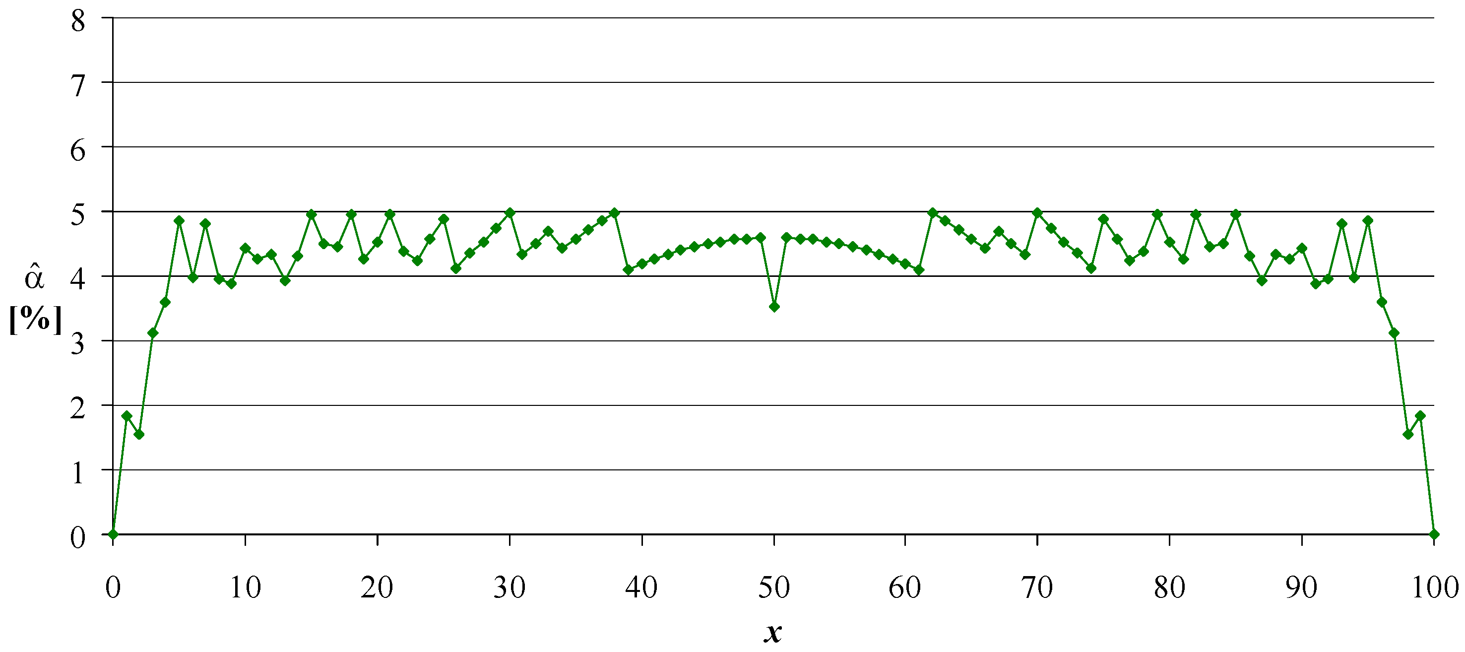
In any study, but especially in medical studies [25], it is more important to ensure that the risk of being in error does not surpass the imposed value. If it surpasses it, we must ensure that it is the smallest value possible. The true coverage probability that the interval contains x is plotted against nominal coverage probability (expected or imposed probability that the interval contains x) to show the performances of the confidence interval method. Figure 1 (see also Figure 3 in [26] and Figure 5 in [12]) illustrate the non-coverage probabilities for Wald confidence interval (CI) based on Equation (5).

$$C{I}_{\mathrm{N}}=[x-\kappa \sqrt{x(m-x)/m},x+\kappa \sqrt{x(m-x)/m}],\kappa =InvCDF(“\mathrm{Normal}”,1-\alpha /2)$$

(5)

For m = 100 the “standard” (or “Wald”; “asymptotic interval”, “no continuity correction”). If $ϵ=\widehat{\alpha }-\alpha$ is the error, then its standard error, SE($ϵ$) is 0.119.

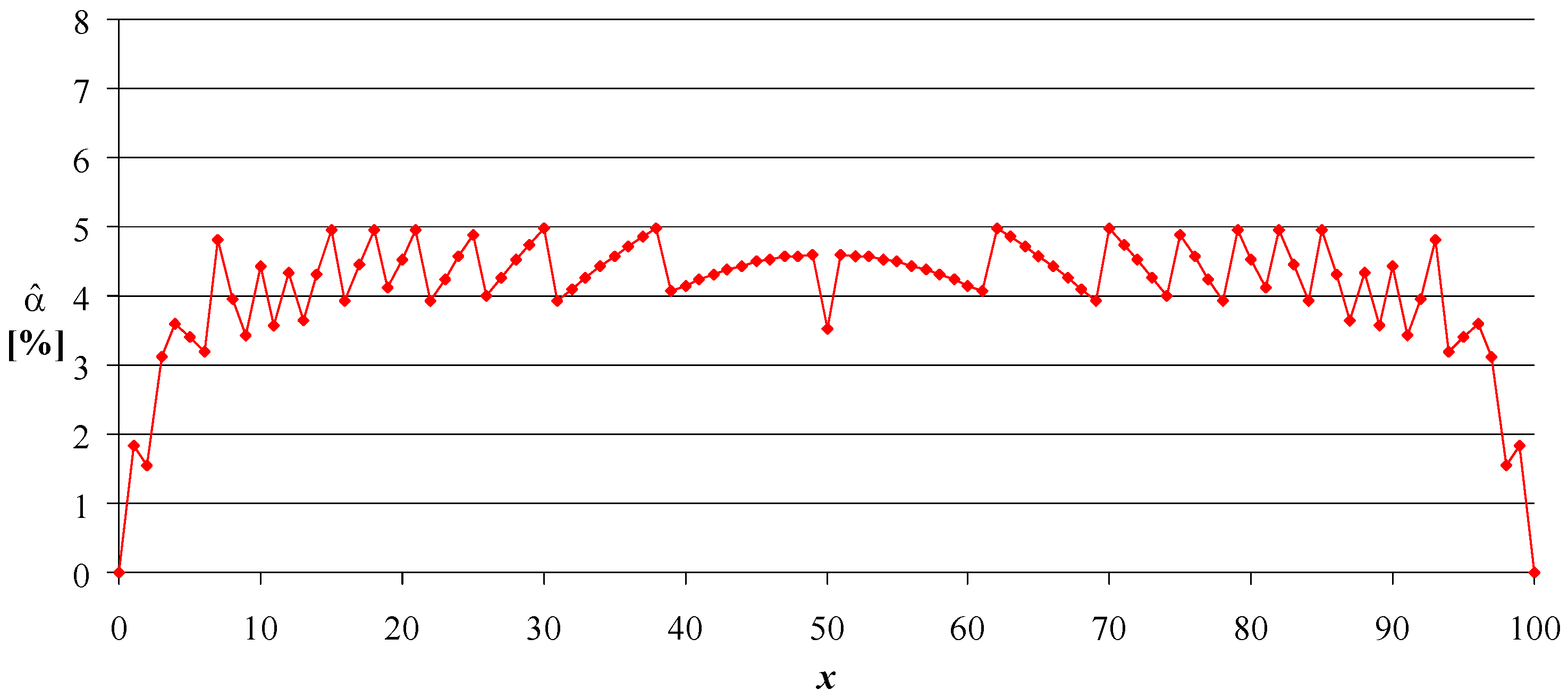
Figure 2, Figure 3 and Figure 4 illustrates “exact method” with different algorithms at the same specific significance level ($\alpha$ = 5%) and number of trials (m = 100).

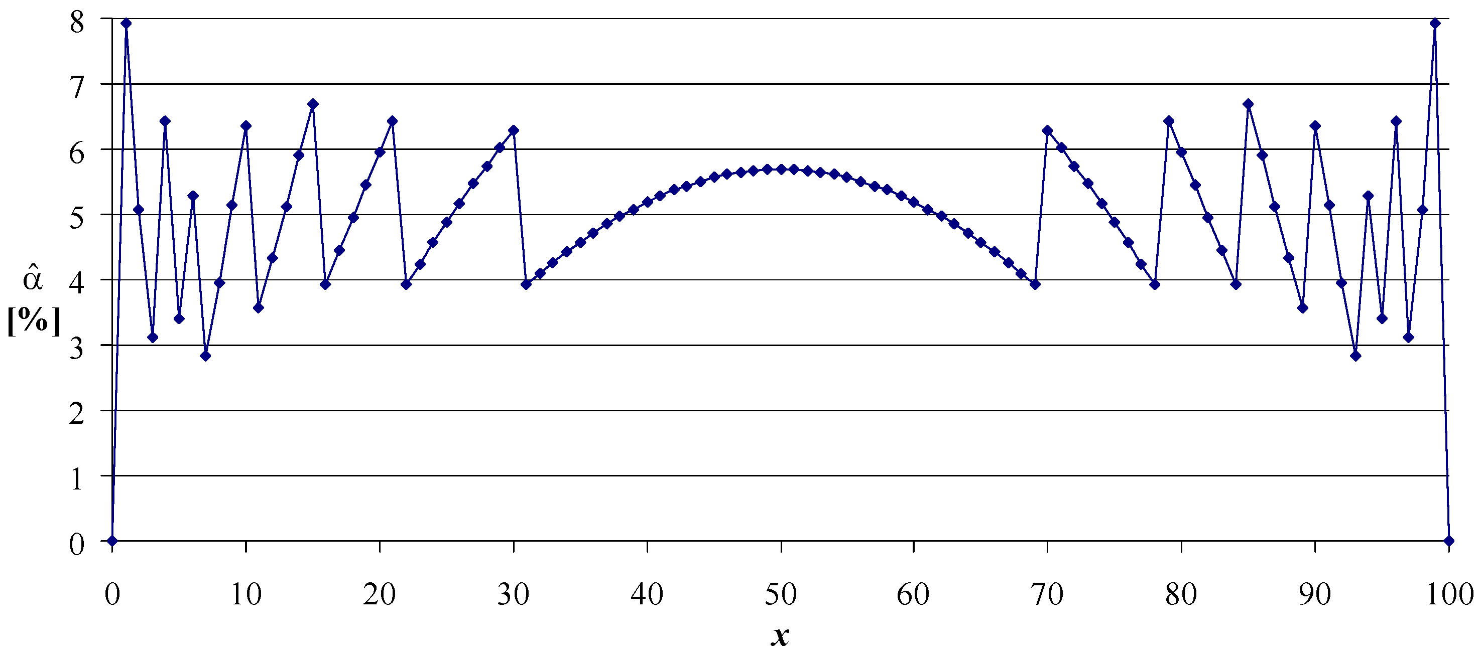
Each of the proposed alternatives (see Figure 3 and Figure 4) is, in a way, an improvement of the normal approximation interval (Equation (5); Figure 3 in [26]; Figure 1 here). Thus, for the actual non-coverage probability ($\widehat{\alpha }$, in %) when $\alpha$ = 5% is the imposed level, m = 100 and x = 0, 1, …, m:

• Figure 1 (asymptotic interval) illustrates $\widehat{\alpha }$ for CI from Equation (5).
• In Figure 2, using CI from Algorithm 1, always $\widehat{\alpha }\le \alpha$ (x = 0, 1, …, m) and SE($ϵ$) = 0.127.
• Figure 1 and Figure 3 (the solutions given by Equation (5) and Algorithm 2) are similar in shape but the amplitude of the oscillation is reduced (SE($ϵ$) from 0.119 to 0.099).
• In Figure 4 (from Algorithm 3) again $\widehat{\alpha }\le \alpha$, and SE($ϵ$) = 0.117 is lower than from Algorithm 1 (0.127).

All proposed methods, as well as the classical Wald method provide symmetry (relative to the middle, p = 0.5, x = 50 on Figure 1, Figure 2, Figure 3 and Figure 4 depicting the true error for a sample of size m = 100). Figure 3 shows a visible improvment in the variation of the error around its imposed level (of 5% in Figure 1, Figure 2, Figure 3 and Figure 4). The solution depicted in Figure 4 is an improvement of the solution depicted in Figure 2 as it has a lower variation of error arround its imposed level.

Althrough providing an accurately calculated confidence interval may closely show what is happening in the population, most researchers are still reticent to use the “exact methods” when caculating confidence intervals. Reputed statisticians suggest that ’approximate is better than exact’ [27]. A better argument for not using the “exact methods” is the complexity of the calculation [21]. The people developing such a method and the researchers supposed to use it are not the same and do not have the same background. In this article, we propose three exact alternatives for calculating the confidence interval to slightly alleviate this inconvenience, examples and illustrations accompany these alternatives.

Following the pattern described by Jäntschi [21] (see Section 5.2 in [21]; the methodology does not change when the distribution is changed), the applied methodology is:

• Collect all possible drawings and their associated probabilities ($(u,f_{\mathrm{RB}}(u;x,m))$ from Equation (3);
• The values (u) are already sorted (and grouped) when u ranges increasingly from 0 to m and the probability mass function (PMF) is defined by the $\{f_{\mathrm{RB}}(0;x,m)$, $f_{\mathrm{RB}}(1;x,m)$, …, $f_{\mathrm{RB}}(u;x,m)$, …, $f_{\mathrm{RB}}(m;x,m)\}$ set;
• Construct cumulative distribution function (CDF; the result is formally defined by Equation (6)) and (from which) CI in increasing coverage for which the result is formally defined by Equation (7)).

$$(u,F_{\mathrm{RB}}(u;x,m)),\mathrm{where}{F}_{\mathrm{RB}}(u;x,m)\leftarrow \sum _{i=0}^u{f}_{\mathrm{RB}}(i;x,m)$$

(6)

$$CI(i_1,i_2)=[x-i_1,x+i_2];pCI(i_1,i_2)=\sum _{i=x-i_1}^{x+i_2}{f}_{\mathrm{RB}}(i;x,m)$$

(7)

One should notice that the methodology is straightforward and easy to follow, even for a non-specialist. The three proposed alternatives are given when a certain interval needs to be chosen.

Proposed CI Calculation Algorithms

Additionally, one can inspect, for instance, the plots from Figure 2 (solution obtained with Algorithm 1), Figure 3 (solution obtained with Algorithm 2), and Figure 4 (solution obtained with Algorithm 3), or the entries in

Table 1. Alternate CIs for replica ($u,m$) of ($x,m$) draw.

$\mathit{C}\mathit{I}({\mathit{i}}_1,{\mathit{i}}_2)$	$\mathit{p}\mathit{C}\mathit{I}({\mathit{i}}_1,{\mathit{i}}_2)$	Strategy
$[1,7]$	0.9817	Descending probabilities (foundational strategy)
$[2,7]$	0.9414	1st Improvement—decrease such that: $|\alpha -pCI|\to min.$
$[2,8]$	0.9520	2nd Improvement—increase such that: $|\alpha -pCI|\to min.$

The first CI of (x = 4, m = 10) (is constructed by inclusion of the likelihood values (f_RB(u; 4, 10)) in a decreasing order. The 1st improvement proposes a shorter interval with a non-coverage probability (1 − 0.9414 = 0.0586) greater than the imposed level (0.0500), but with a much better proximity to it (1 − 0.9817 = 0.0183). The 2nd improvement expands the 1st improvement and provides an even better proximity (1 − 0.9520 = 0.0480).

(where $[1,7]$ is obtained with Algorithm 1, $[2,7]$ is obtained with Algorithm 2 and $[2,8]$ with Algorithm 3).

Algorithm 1: Foundational confidence interval, CI_v0

Input: $\alpha$, x, m    //imposed level, number of successes, number of trials   procedureFound($\beta ,x,m,\&r,\&i,\&j,\&q$)      $i\leftarrow x$; $j\leftarrow x$; $q\leftarrow r\left[x\right]$      For( ; ; )         if($q\ge \beta$) Break; if($(i=0)$ AND $(j=m)$) Break         If($i=0$) $j\leftarrow j+1$; $q\leftarrow q+r\left[j\right]$; Continue EndIf         If($j=m$) $i\leftarrow i-1$; $q\leftarrow q+r\left[i\right]$; Continue EndIf         If($r[i-1]=r[j+1]$) $i\leftarrow i-1$; $j\leftarrow j+1$; $q\leftarrow q+r\left[i\right]+r\left[j\right]$; Continue EndIf         If($r[i-1]>r[j+1]$) $i\leftarrow i-1$; $q\leftarrow q+r\left[i\right]$; Continue EndIf         If($r[i-1]<r[j+1]$) $j\leftarrow j+1$; $q\leftarrow q+r\left[j\right]$; Continue EndIf      EndFor   end procedure   procedureCI_v0($\alpha ,x,m,\&i1,\&i2,\&q$)     PMF_B($x,m,r$); $\beta \leftarrow 1-\alpha$; Found($\beta ,x,m,r,i1,i2$)   end procedure Output:$i1$, $i2$, q    // $[i1,i2]$ is the CI; q is the actual CI’s coverage

Algorithm 2: First improved confidence interval, CI_v1

Input: $\alpha$, x, m    imposed level, number of successes, number of trials   procedureImp_1($\beta ,x,m,\&r,\&i,\&j,\&q$)      For( ; ; )         if( $j\le i$ ) Break         If( $r\left[i\right]=r\left[j\right]$ )            If( Abs($\beta -q$) > Abs($\beta -q+r\left[i\right]+r\left[j\right]$) )               $q\leftarrow q-r\left[i\right]-r\left[j\right]$; $i\leftarrow i+1$; $j\leftarrow j-1$            EndIf            Break         EndIf         If( $r\left[i\right]<r\left[j\right]$ )            If( Abs($\beta -q$) > Abs($\beta -q+r\left[i\right]$) ) $q\leftarrow q-r\left[i\right]$; $i\leftarrow i+1$; EndIf            Break         EndIf         If( $r\left[i\right]>r\left[j\right]$ )            If( Abs($\beta -q$) > Abs($\beta -q+r\left[j\right]$) ) $q\leftarrow q-r\left[j\right]$; $j\leftarrow j-1$ EndIf            Break         EndIf      EndFor   end procedure   procedureCI_v1($\alpha$, x, m, i1, i2, er)      PMF_B($x,m,r$); $\beta \leftarrow 1-\alpha$; Found($\beta ,x,m,r,i1,i2$); Imp_1($\beta ,x,m,r,i1,i2,q$)   end procedure Output: $i1$, $i2$, q    // $[i1,i2]$ is the CI; q is the actual CI’s coverage

Algorithm 3: Second improved confidence interval, CI_v2

Input: $\alpha$, x, m    imposed level, number of successes, number of trials   procedureImp_2($\beta ,x,m,\&r,\&i,\&j,\&q$)      For( ; ; )         if($q\ge \beta$) Break; if($(i=0)$ AND $(j=m)$) Break         If($i=0$) $j\leftarrow j+1$; $q\leftarrow q+r\left[j\right]$; Continue EndIf         If($j=m$) $i\leftarrow i-1$; $q\leftarrow q+r\left[i\right]$; Continue EndIf         If($r[i-1]=r[j+1]$) $i\leftarrow i-1$; $j\leftarrow j+1$; $q\leftarrow q+r\left[i\right]+r\left[j\right]$; Continue EndIf         If($r[i-1]<r[j+1]$) $i\leftarrow i-1$; $q\leftarrow q+r\left[i\right]$; Continue EndIf         If($r[i-1]>r[j+1]$) $j\leftarrow j+1$; $q\leftarrow q+r\left[j\right]$; Continue EndIf      EndFor   end procedure   procedureCI_v2($\alpha$, x, m, i1, i2, er)      PMF_B($x,m,r$); $\beta \leftarrow 1-\alpha$; Found($\beta ,x,m,r,i1,i2$)      Imp_1($\beta ,x,m,r,i1,i2,q$); Imp_2($\beta ,x,m,r,i1,i2,q$)   end procedure Output:$i1$, $i2$, q    // $[i1,i2]$ is the CI; q is the actual CI’s coverage

5. Results and Discussion

Consider one example ($m=10$ and $x=4$) and follow the methodology described above until Equation (7).

Table 2. PMF example for a replica ($u,m$) of a ($x,m$) draw ($f_{\mathrm{RB}}$ from Equation (3)).

u	${\mathit{f}}_{\mathbf{RB}}\left(\mathit{u};4,10\right)$	u	${\mathit{f}}_{\mathbf{RB}}\left(\mathit{u};4,10\right)$
0	0.0060	6	0.1115
1	0.0403	7	0.0425
2	0.1209	8	0.0106
3	0.2150	9	0.0016
4	0.2508	10	0.0001
5	0.2007	Any	1.0000

PMF for (u, m = 10) resampling (with replacement) of (x = 4, m = 10) is given {(u, f_RB(u; 4, 10)), 0 ≤ u ≤ 10}. It can be observed that u = x is the most probable event. The numeric values of the probabilities are given with four significant decimals. However, the calculations and the actual values are recommended to be done with machine-like precision (see Table 2 in [4] and Section 5.3 in [21] for an extended explanation).

contains all possible outcomes (sampling with replacement) from the population when $m=10$ drawn had $x=4$ successes.

Table 3. CDF example for a replica ($u,m$) of a ($x,m$) draw ($F_{\mathrm{RB}}$ from Equation (6)).

u	${\mathit{F}}_{\mathbf{RB}}\left(\mathit{u};4,10\right)$	u	${\mathit{F}}_{\mathbf{RB}}\left(\mathit{u};4,10\right)$
0	0.0060	6	0.9452
1	0.0463	7	0.9877
2	0.1672	8	0.9983
3	0.3822	9	0.9999
4	0.6330	10	1.0000
5	0.8337

CDF for (u, m = 10) resampling (with replacement) of (x = 4, m = 10) is given {(u, f_RB(u; 4, 10)), 0 ≤ u ≤ 10}.

contains the cumulative distribution function (CDF; Equation (6)) for the data from Table 2.

Table 4. CIs for any replica ($u,m$) of a ($x,m$) draw ($C{I}_{i_1,i_2}$ from Equation (7)).

${\mathit{i}}_1$	${\mathit{i}}_2$	$\mathit{C}\mathit{I}({\mathit{i}}_1,{\mathit{i}}_2)$	$\mathit{p}\mathit{C}\mathit{I}({\mathit{i}}_1,{\mathit{i}}_2)$	${\mathit{i}}_1$	${\mathit{i}}_2$	$\mathit{C}\mathit{I}({\mathit{i}}_1,{\mathit{i}}_2)$	$\mathit{p}\mathit{C}\mathit{I}({\mathit{i}}_1,{\mathit{i}}_2)$
4	4	[4, 4]	0.2508	1	7	[1, 7]	0.9817
3	4	[3, 4]	0.4658	1	8	[1, 8]	0.9923
3	5	[3, 5]	0.6665	0	8	[0, 8]	0.9983
2	5	[2, 5]	0.7874	0	9	[0, 9]	0.9999
2	6	[2, 6]	0.8989	0	10	[0, 10]	1
2	7	[2, 7]	0.9414

CI for any (u, m = 10) resampling (with replacement) of (x = 4, m = 10) is constructed by inclusion in decreasing value of the likelihood (f_RB(u; 4, 10)). The values of the probabilities are given with four significant decimals.

lists true coverage probabilities for the same primary data in Table 2, as the final step (from the CDF given in Table 3) in the common strategy providing the CI (Equation (7)).

As Table 4 reveals, the construction of the confidence interval follows the same strategy as the one used for CDF (from Table 3; $F_{\mathrm{RB}}(u;x,m)=P(u\le x)$, $pCI(i_1,i_2)=P(i_1\le u\le i_2)$) but in the calculation of CI the CDF is not particularly effective ($pCI(i_1,i_2)=P(u\le i_2)-P(u<i_1)$); a more direct approach is from PMF. The construction of the CI from the draws sorted in descending order of likelihood is the choice making more sense for me (Bayesian reasoning; see [28] for the foundations of Bayesian reasoning and [29] for more details on Bayesian reasoning).

The solution presented in Table 4 is the simplest way to construct CI (Crow was probably the first that proposed the construction of the CI in this manner [23]) but it is merely one alternative. To exemplify, the proposed example should be reconsidered (with $x=4$ and $m=10$) for an imposed level (of non-coverage) $\alpha$ = 0.05. Table (Table 1) presents three alternatives.

The 2nd strategy exemplified in Table 1 should operate on the $CI$ provided by the foundational (1st) strategy and try to improve it by narrowing it, i.e., by trying to increase the lower boundary and trying to decrease the upper boundary such that $|\alpha -pCI|$ is minimized. Similarly, 3rd strategy exemplified in Table 1 try to improve the 2nd strategy by broader it (operate to decreases the lower bound and to increase the upper bound such that $|\alpha -pCI|$ is minimized).

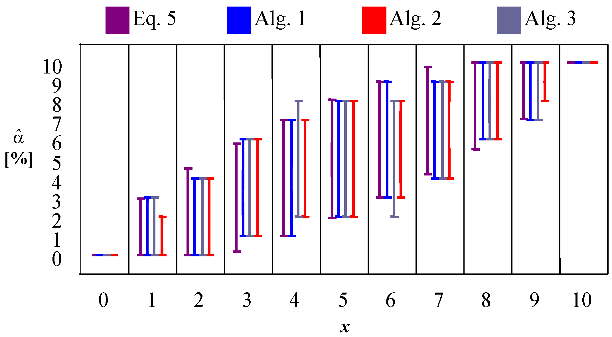
PMF for a binomial distribution is calculated with Algorithm 1 from [21]. By calling PMF_B$\left(x,m,r\right)$ the output r is an array indexed from 0 to m and containing the series of probabilities from Equation (3). There are differences between the solutions proposed by the Algorithm 1–3 algorithms (see Figure 5).

5.1. Properties of the Proposed Solutions

Each proposed solution is (anti)symmetrical, not relatively to the observed successes but relatively to its complement compared to half. Specifically, if $[i_1,i_2]$ is the CI of x successes from m draws, then $[m-i_1,m-i_2]$ is the CI of $m-x$ successes from m draws. This property is available for the normal approximation interval as well (Equation (5)). It can be easily checked that if $C{I}_{\mathrm{N}}\left(x\right)=[CI{L}_N\left(x\right),CI{U}_N\left(x\right)]=[x-\kappa \sqrt{x(m-x)/m},x+\kappa \sqrt{x(m-x)/m}]$ (see Equation (5)), then substituting x with $m-x$, $C{I}_{\mathrm{N}}(m-x)=[CI{L}_N(m-x),CI{U}_N(m-x)]=[m-x-\kappa \sqrt{x(m-x)/m},m-x+\kappa \sqrt{x(m-x)/m}]$ and $CI{L}_N(m-x)$ + $CI{U}_N\left(x\right)$ = m = $CI{U}_N(m-x)$ + $CI{L}_N\left(x\right)$ and the actual coverage probability is the same (see Figure 1, Figure 2, Figure 3 and Figure 4; all are symmetrical). When considering the proposed solutions (Algorithms 1–3) the (anti)symmetry is kept due to the presence of the If(r[i-1]=r[j+1])…EndIf (Algorithms 1 and 3), and If(r[i]=r[j])…EndIf (Algorithm 2) instructions blocks. Additionally, an important remark could be made about the Normal approximation interval (Equation (5)). This interval is actually (as defined by Equation (5)) even more symmetrical in relation to the observed number of successes (x), but if anyone considers the confidence intervals proposed by Equation (5) to be a very small (such as is x = 1, 2, …) or very large (such as is x = $m-1$, $m-2$, …) number of successes (see

Table 5. Patching the normal CIs for binomial data.

x	$1-\mathbf{pCI}\left(\mathit{x}\right)$	${\mathit{C}\mathit{I}}_{\mathit{N}}\left(\mathit{x}\right)$	${\mathit{C}\mathit{I}}_{\mathit{N}\mathit{P}}\left(\mathit{x}\right)$	${\mathit{C}\mathit{I}}_{\mathit{N}\mathit{N}}\left(\mathit{x}\right)$
1	0.0702	[−0.9$,+2.9]$	$[0.0,2.9]$	$[0,2]$
2	0.0328	[−0.5$,+4.5]$	$[0.0,4.5]$	$[0,4]$
3	0.0756	$[+0.2,+5.8]$	$[0.2,5.8]$	$[1,5]$
7	0.0756	$[+4.2,+9.8]$	$[4.2,9.8]$	$[4,9]$
8	0.0328	$[+5.5,10.5]$	$[5.5,10.0]$	$[5,10]$
9	0.0702	$[+7.1,10.9]$	$[7.1,10.0]$	$[7,10]$

In this case, patching is exemplified for α = 0.05, m = 10 and x = 0, 1, 2. Coverage probability (pCI(x)) is not changed due to patching. CI_N(x) is the CI calculated with Equation (5); one decimal digit is given. Since only an integer between 0 and m = 10 can be recorded as number of successes, CI_NP(x) is the adjustment of the CI calculated with Equation (5) and adjusted to make sense at limits (0 and m = 10); one decimal digit is given. Furthermore, since only a natural number of successes can be recorded, a decimal number as boundary may be implausible, so CI_NP(x) is the adjustment of the CI_NP(x) to have integer boundaries.

), it will be seen that a bound greater than m or smaller than 0 is not logical; therefore, it must be immediately patched (Equation 8).

$$C{I}_{NP}(x,m,\alpha )=[\max (0,CI{L}_N(x,m,\alpha )),\min (m,CI{U}_N(x,m,\alpha ))]$$

(8)

All integer boundaries formulas (column $C{I}_{N}N\left(x\right)$ in Table 5) can be easily obtained (Equation (9), where $\lceil ·\rceil$ is the ceil function and $\lfloor ·\rfloor$ is the floor function) from Equation (8).

$$C{I}_{NN}(x,m,\alpha )=[\lceil CI{L}_{NP}(x,m,\alpha )\rceil ,\lfloor CI{U}_{NP}(x,m,\alpha )\rfloor ]$$

(9)

$C{I}_{NP}(x,m,\alpha )$ and $C{I}_{NN}(x,m,\alpha )$ possess exactly the same (anti)symmetrical properties like the proposed ones (Algorithms 1–3).

A consequence derives from this property: it is sufficient to know one bound for all range of successes in order to know the other bound as well. For convenience, three series are listed in the Appendix A (

Table A1. Numbers providing the confidence intervals from Algorithm 1 at $\alpha$ = 0.05: $CI(\alpha ,x,m)=[N_x,m-N_{m-x}]$.

m	+	+	+	20	19	18	17	16	15	14	13	12	11	10	9	8	7	6	5	4	3	2	1	0	x
1	0	1	+	20	17	16	14	13	11	10	9	8	7	6	5	4	3	2	2	1	0	0	0	0	20
2	0	0	2	+	19	16	15	13	12	10	9	8	7	6	5	4	3	3	2	1	0	0	0	0	19
3	0	0	1	3	+	18	15	14	12	11	9	8	7	6	5	4	3	3	2	1	0	0	0	0	18
4	0	0	0	1	4	+	17	14	13	11	10	8	7	6	5	4	3	3	2	1	0	0	0	0	17
5	0	0	0	1	2	5	+	16	13	12	10	9	7	6	5	4	4	3	2	1	0	0	0	0	16
6	0	0	0	1	2	3	6	+	15	12	11	9	8	6	5	4	4	3	2	1	0	0	0	0	15
7	0	0	0	1	2	3	4	7	+	14	11	10	8	7	6	4	3	3	2	1	0	0	0	0	14
8	0	0	0	1	1	2	4	5	8	+	13	10	9	7	6	5	4	3	2	1	1	0	0	0	13
9	0	0	0	1	2	2	3	5	6	9	+	12	9	8	6	5	4	3	2	1	1	0	0	0	12
10	0	0	0	1	1	2	3	4	6	7	10	+	11	8	7	5	4	3	2	1	1	0	0	0	11
x	0	1	2	3	4	5	6	7	8	9	10	+	+	+	+	+	+	+	+	+	+	+	+	+	m

,

Table A2. Numbers providing the confidence intervals from Algorithm 2 at $\alpha$ = 0.05: $CI(\alpha ,x,m)=[N_x,m-N_{m-x}]$.

m	+	+	+	20	19	18	17	16	15	14	13	12	11	10	9	8	7	6	5	4	3	2	1	0	x
1	0	1	+	20	18	16	14	13	11	10	9	8	7	6	5	4	4	3	2	1	1	0	0	0	20
2	0	0	2	+	19	17	15	13	12	11	9	8	7	6	5	4	4	3	2	1	1	0	0	0	19
3	0	0	1	3	+	18	16	14	12	11	10	8	7	6	5	5	4	3	2	1	1	0	0	0	18
4	0	0	0	2	4	+	17	15	13	11	10	9	7	6	5	5	4	3	2	1	1	0	0	0	17
5	0	0	0	2	3	5	+	16	14	12	10	9	8	6	5	5	4	3	2	1	1	0	0	0	16
6	0	0	0	1	2	4	6	+	15	13	11	9	8	7	6	4	4	3	2	1	1	0	0	0	15
7	0	0	0	1	2	3	5	7	+	14	12	10	8	7	6	5	4	3	2	1	1	0	0	0	14
8	0	0	0	1	2	3	4	6	8	+	13	11	9	7	6	5	4	3	2	1	1	0	0	0	13
9	0	0	0	1	2	2	3	5	7	9	+	12	10	8	6	5	4	3	2	2	1	0	0	0	12
10	0	0	0	1	2	2	3	4	6	8	10	+	11	9	7	5	4	3	2	2	1	0	0	0	11
x	0	1	2	3	4	5	6	7	8	9	10	+	+	+	+	+	+	+	+	+	+	+	+	+	m

and

Table A3. Numbers providing the confidence intervals from Algorithm 3 at $\alpha$ = 0.05: $CI(\alpha ,x,m)=[N_x,m-N_{m-x}]$.

m	+	+	+	20	19	18	17	16	15	14	13	12	11	10	9	8	7	6	5	4	3	2	1	0	x
1	0	1	+	20	17	16	13	13	11	9	7	8	7	6	5	4	4	3	2	1	1	0	0	0	20
2	0	0	2	+	19	16	15	12	12	11	9	7	7	6	5	4	4	3	1	1	1	0	0	0	19
3	0	0	1	3	+	18	15	14	11	11	10	8	6	5	5	5	4	3	1	1	1	0	0	0	18
4	0	0	0	1	4	+	17	14	13	10	10	9	7	5	4	5	4	3	1	1	1	0	0	0	17
5	0	0	0	1	2	5	+	16	13	12	9	9	8	6	5	4	4	3	1	1	1	0	0	0	16
6	0	0	0	1	2	3	6	+	15	12	11	8	8	7	6	4	4	2	1	1	1	0	0	0	15
7	0	0	0	1	2	3	4	7	+	14	11	10	7	7	6	5	3	2	2	1	1	0	0	0	14
8	0	0	0	0	1	3	4	5	8	+	13	10	9	7	6	5	4	3	2	1	1	0	0	0	13
9	0	0	0	1	2	2	3	5	6	9	+	12	9	8	6	0	4	3	2	1	1	0	0	0	12
10	0	0	0	1	2	2	2	4	6	7	10	+	11	8	7	5	0	3	2	1	1	0	0	0	11
x	0	1	2	3	4	5	6	7	8	9	10	+	+	+	+	+	+	+	+	+	+	+	+	+	m

) of lower boundaries for the proposed CI alternatives. In each case, if ${\left(N_i\right)}_{0\le i\le m}$ is the series given, then the confidence interval of $x=i$ is $[N_i,m-N_{m-i}]$. Each table presents the run of one algorithm, so the solution proposed by individual algorithms (Table A1 for Algorithm 1, Table A2 for Algorithm 2, and Table A3 for Algorithm 3). The algorithms were implemented in PHP language and the outputs are given. There is no serious constraint in the computation, other than memory limits of the computer; see Section 5.3 for details. An example is suitable here. It would be useful to know the smallest sample size for which the proposed algorithms provide different solutions. That is $m=8$. The CI calculated from the $N_i$ numbers are given in

Table 6. Example of distinct solutions proposed by the algorithms.

Bin	${\mathit{N}}_{\mathit{i}}$			CI			$\widehat{\mathit{\alpha }}$, in %
0	0	0	0	[0, 0]	[0, 0]	[0, 0]	0.00	0.00	0.00
1	0	0	0	[0, 3]	[0, 2]	[0, 3]	1.12	6.73	1.12
2	0	0	0	[0, 4]	[0, 4]	[0, 4]	2.73	2.73	2.73
3	1	1	0	[1, 6]	[1, 5]	[0, 5]	2.89	5.93	3.60
4	1	2	1	[1, 7]	[2, 6]	[1, 7]	0.78	7.03	0.78
5	2	3	3	[2, 7]	[3, 7]	[3, 8]	2.89	5.93	3.60
6	4	4	4	[4, 8]	[4, 8]	[4, 8]	2.73	2.73	2.73
7	5	6	5	[5, 8]	[6, 8]	[5, 8]	1.12	6.73	1.12
8	8	8	8	[8, 8]	[8, 8]	[8, 8]	0.00	0.00	0.00
x	A1	A2	A3	A1	A2	A3	A1	A2	A3

It should be noted that the proposed solutions corresponds to m = 8 and α = 5%, so the expected value for each entry in $\widehat{\mathit{\alpha }}$ column is 5.00%.

.

Please note that when m is very small the whole probability space is small (Equation (3) defines a $(m+1)\times (m+1)$ matrix) so any method (optimized or not) have to choose from a very small set of possibble choices. This peculiar behavior is visible in the Appendix A Table A1, Table A2, Table A3 and

Table A4. Numbers providing the confidence intervals with monotonic boundaries constrain at $\alpha$ = 0.05: $CI(\alpha ,x,m)=[N_x,m-N_{m-x}]$.

m∖x	0	1	2	3	4	5	6	7	8	9	10	11	12	13	14	15	16	17	18	19	20	21	22	23	24	25	26	27	28	29	30	31
2	0	0	2
3	0	0	1	3
4	0	0	0	2	4
5	0	0	0	2	3	5
6	0	0	0	1	2	4	6
7	0	0	0	1	2	3	5	7
8	0	0	0	1	2	3	4	6	8
9	0	0	0	0	2	2	4	5	7	9
10	0	0	0	0	2	2	2	5	6	8	10
11	0	0	0	0	2	2	2	2	6	7	9	11
12	0	0	0	0	2	2	2	2	2	7	8	10	12
13	0	0	0	0	2	2	2	2	2	2	8	9	11	13
14	0	0	0	0	2	2	2	2	2	2	2	9	10	12	14
15	0	0	0	0	2	2	2	2	2	2	2	2	10	11	13	15
16	0	0	0	0	1	2	2	2	2	2	2	2	9	11	12	14	16
17	0	0	0	0	1	2	2	2	2	2	2	2	9	10	12	13	15	17
18	0	0	0	0	1	1	2	2	2	2	2	2	9	10	11	13	14	16	18
19	0	0	0	0	1	1	2	2	2	2	2	2	9	10	11	12	14	15	17	19
20	0	0	0	0	1	1	1	2	2	2	2	2	9	10	11	12	13	15	16	18	20
21	0	0	0	0	1	1	1	1	2	2	2	2	9	10	11	12	13	14	16	17	19	21
22	0	0	0	0	1	1	1	1	1	2	2	2	9	10	11	12	13	14	15	17	18	20	22
23	0	0	0	0	1	1	1	1	1	1	2	2	8	9	11	12	13	14	15	16	18	19	21	23
24	0	0	0	0	1	1	1	1	1	1	2	2	8	9	10	11	13	14	15	16	17	19	20	22	24
25	0	0	0	0	1	1	1	1	1	1	2	2	7	9	10	11	12	14	15	16	17	18	20	21	23	25
26	0	0	0	0	1	1	1	1	1	1	2	2	7	8	10	11	12	13	14	16	17	18	19	21	22	24	26
27	0	0	0	0	1	1	1	1	1	1	2	2	6	7	10	11	12	13	14	15	17	18	19	20	22	23	25	27
28	0	0	0	0	1	1	1	1	1	1	2	2	6	7	9	11	12	13	14	15	16	18	19	20	21	23	24	26	28
29	0	0	0	0	1	1	1	1	1	1	2	2	6	6	7	11	12	13	14	15	16	17	18	20	21	22	24	25	27	29
30	0	0	0	0	1	1	1	1	1	1	2	2	5	6	6	10	12	13	14	15	16	17	18	19	21	22	23	25	26	28	30
31	0	0	0	0	1	1	1	1	1	1	2	2	2	5	6	6	12	13	14	15	16	17	18	19	20	22	23	24	26	27	29	31

as well: the entries for $m=2$ and $m=3$ are identical and until $m=8$ it is in one way or another an overlap between the proposed solutions.

5.2. Smoothing of the Proposed Solutions

Smoothing a data set is typically done to create an approximating function that captures important patterns in the data, leaving out noise or other fine-scale variations [30]. In this instance, smoothing is proposed to be used to introduce noise, or a fine-scale variation, to make the confidence interval more similar to the normal approximation (Equation (5); to all intents and purposes like its patch Equation (8). Ergo, someone may say that $C{I}_{NN}$ is the anti-smoothed version of the patched normal approximation confidence interval ($C{I}_{NP}$).

Considering that two adjacent intervals that natively do not intersect will still not intersect after smoothing. It means that, by smoothing, they should not be enlarged with more than a half of 1/m. Also, smoothing should balance the transition from one number of successes (x) to adjacent numbers of successes ($x-1$ and $x+1$). An interval is made with common sense by picking its limits between two integers such that the ratio of the probabilities of their extraction is also the ratio in which the limit divides the allotted distance between them (0.5, Equation (10).

$$\begin{array}{c}\hfill \mathrm{If}[i_1,i_2]\mathrm{non-smoothed}\mathrm{interval},\mathrm{then}[x_1,x_2]\mathrm{smoothed}\mathrm{interval},\mathrm{with}:\\ \hfill x_1=\left\{\begin{array}{c}0,\mathrm{if}{i}_1=0\hfill \\ i_1-0.5\frac{f_{\mathrm{RB}}(i_1,x,m)}{f_{\mathrm{RB}}(i_1,x,m)+f_{\mathrm{RB}}(i_1-1,x,m)}\hfill \end{array}\right.,\mathrm{otherwise}\\ \hfill x_2=\left\{\begin{array}{c}m,\mathrm{if}{i}_2=m\hfill \\ i_2+0.5\frac{f_{\mathrm{RB}}(i_2,x,m)}{f_{\mathrm{RB}}(i_2,x,m)+f_{\mathrm{RB}}(i_2+1,x,m)}\hfill \end{array}\right.,\mathrm{otherwise}\end{array}$$

(10)

Smoothing with Equation (10) does not change the coverage probability (the coverage probabilities of $[i_1,i_2]$ and $[x_1,x_2]$ are equal) because the change is too small, smaller than the increment between the success events.

5.3. General Discussion

What if one follows the (numerous) sets of rules, such as having a confidence interval of which boundaries are monotonic functions? It may be checked that the solutions proposed by Algorithms 1 and 2 are both monotonic (all the data given in Table A1 and Table A2. A screening conducted for m from 21 to 100 also supported the monotony. So, in actuality, two proposed solutions follow some rules (another rule implemented in the algorithm is that the confidence interval is constructed from redrawn successes taken in descending order of the probabilities—most likely first).

The series of numbers giving one boundary may be inspected in more details. Consider the series for m = 25 and $\alpha =0.05$ provided by Algorithm 1: N = {0, 0, 0, 0, 1, 2, 2, 3, 4, 5, 6, 7, 8, 8, 9, 10, 11, 12, 14, 15, 16, 18, 19, 21, 22, 25}. Independently of the algorithm, sample size, and imposed significance level, the first ($N_0$) and last ($N_m$) are known ($N_0$ = 0, $N_m$ = m) as well as actual non-coverage probabilities associated with a $u=0$ and $u=m$ draw (0%, $[0,0]$ and [$m,m$] intervals cover all possible cases, see Equation (3). Since CI is $[N_i,m-N_{m-i}]$ (see Section 5.1) bigger numbers in the series means narrower confidence intervals (the bounds are then closer) while smaller numbers in the series mean larger confidence intervals (the bounds are then farther). This is an important property which allows us to simplify the reasoning.

Nevertheless, someone may argue that this is not enough (see [17] patched in [18]), so what is happening when arbitrary (but with a sort of common sense) rules are imposed (see Equation 1.3 and 1.4 in [17]) should be analyzed. Moving from the CI for m = 25 to the CI for m = 26 (whenever; applicable for any succession), one may argue that the lower bound of the CIs for x successes from $m+1$ draws should not be greater than the bound of the CI for x successes from m draws (the general trend in the columns in Table A1 and Table A2 should be considered). As result, once you have constructed the series of N for $m+1$ from the series of N for m, all that is needed is to add the new sample size ($m+1$) at the end, thus getting a series of bounds which are (the first ones) following the defined rule and may contain numbers generally higher than the desired ones. A such series should be labeled $NS$; $NS$ series for m = 26 and $\alpha =0.05$ is $NS$ = {0, 0, 0, 0, 1, 2, 2, 3, 4, 5, 6, 7, 8, 8, 9, 10, 11, 12, 14, 15, 16, 18, 19, 21, 22, 25, 26}). By following an exactly mirrored reasoning, by adding a 0 at the beginning, the result is a series of too large but still rule complying series. A such series may contain numbers generally smaller than the desired ones and this series should be labeled $NI$ ($NI$ series for m = 26 and $\alpha =0.05$ is $NI$ = {0, 0, 0, 0, 0, 1, 2, 2, 3, 4, 5, 6, 7, 8, 8, 9, 10, 11, 12, 14, 15, 16, 18, 19, 21, 22, 25}).

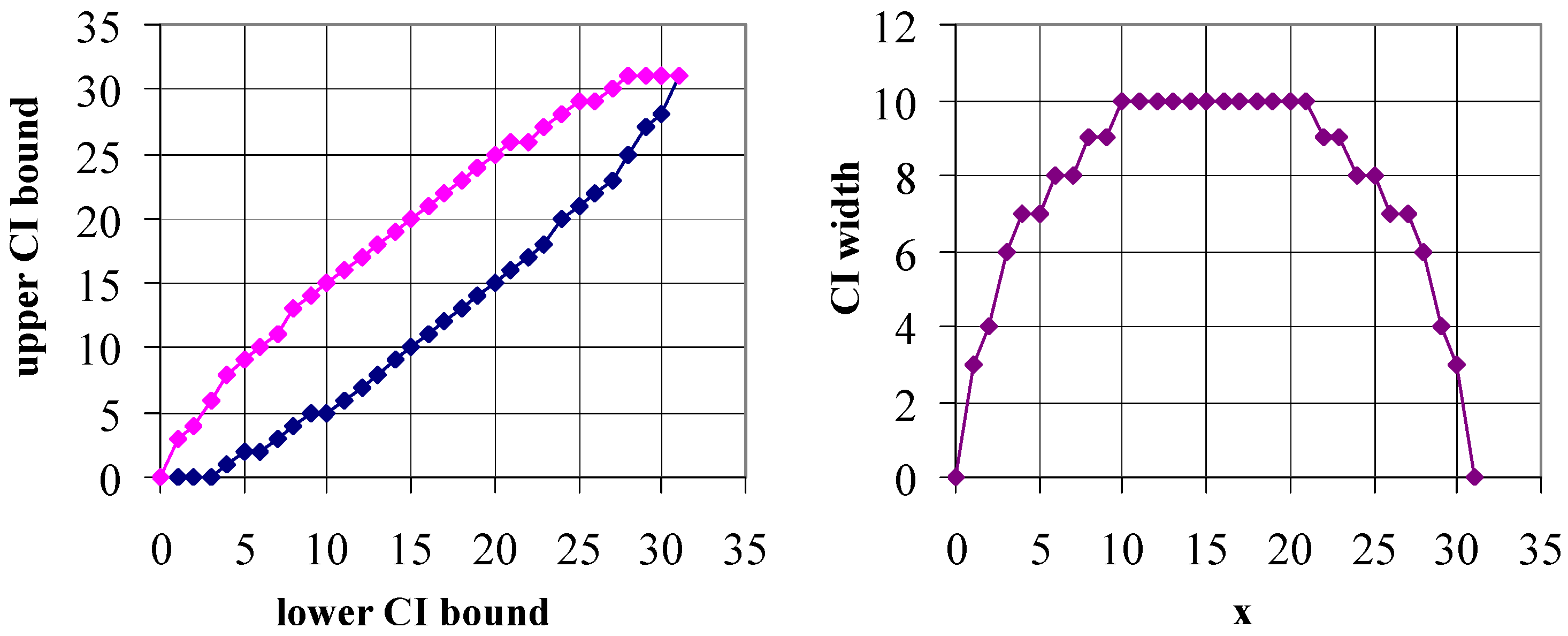
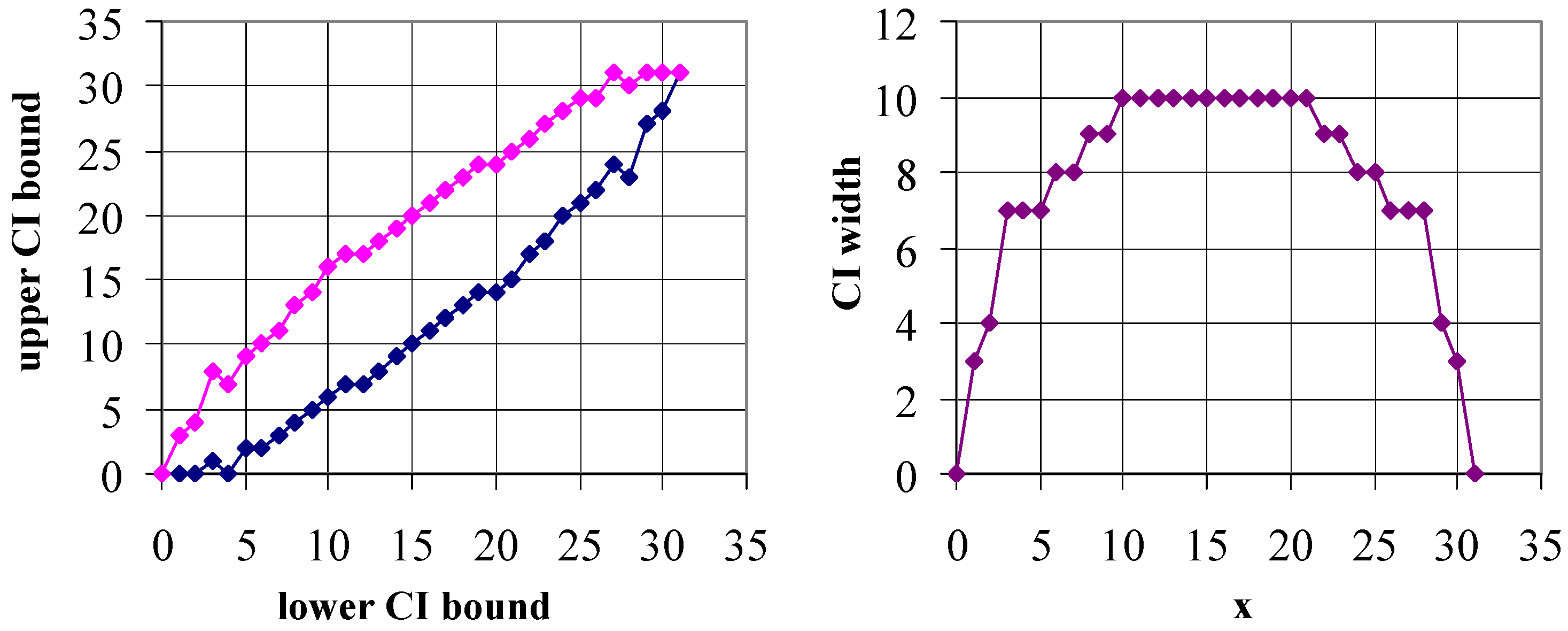
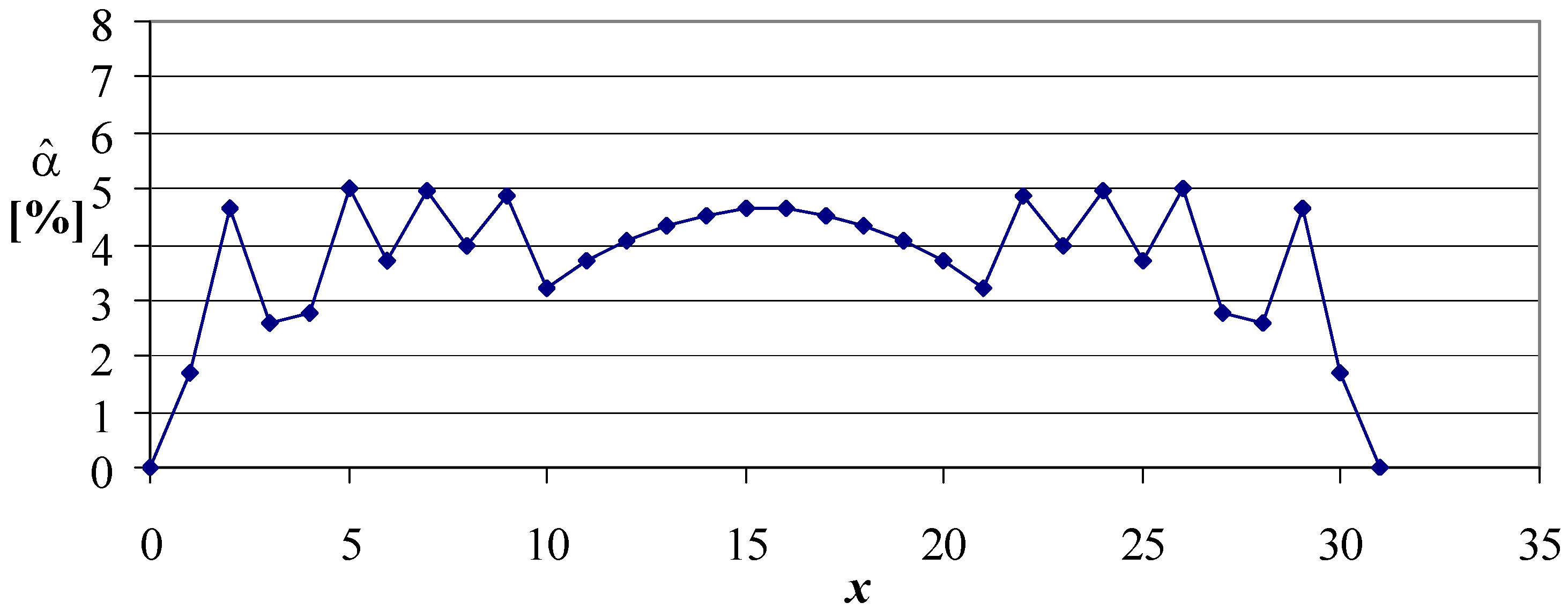
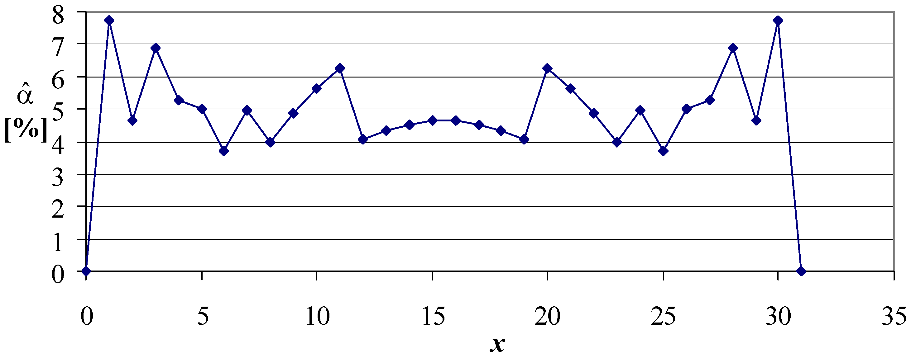
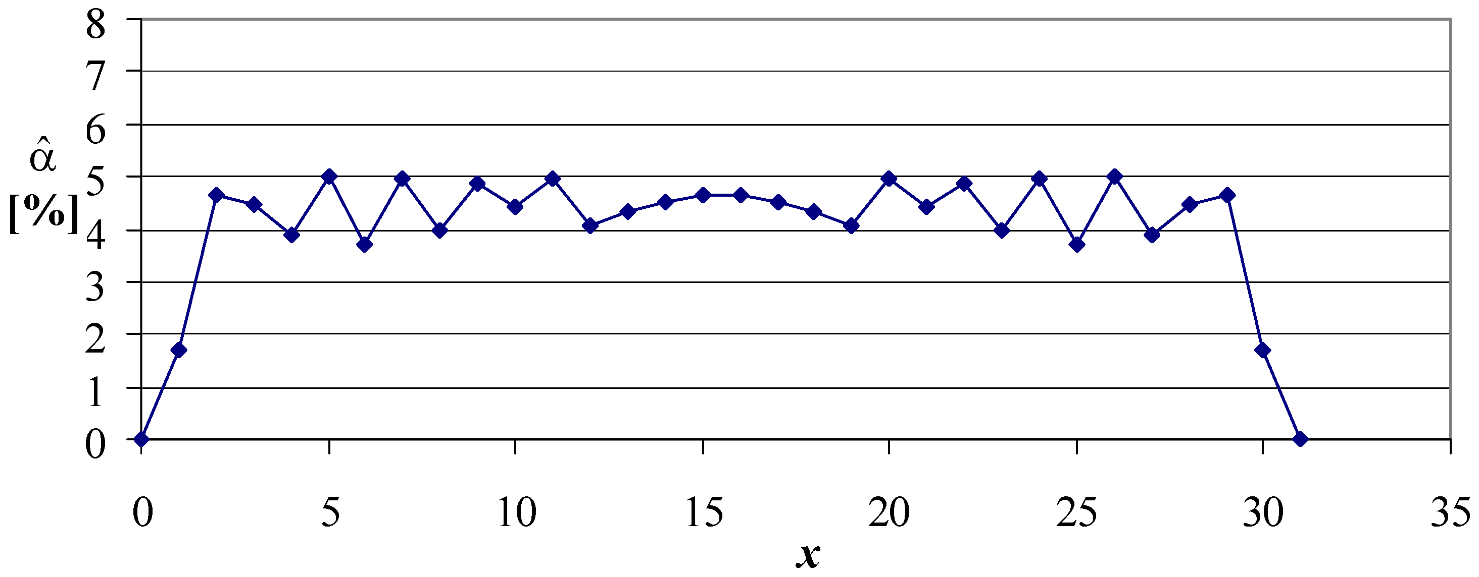
The $NI$ and $NS$ series defines a trap for any confidence interval following an extended monotony rule (if $NN$ is the best option then $N{S}_x\le N{N}_x\le N{I}_x$ for $0\le x\le m$). Why not find the best one? It is a matter of extensive search and the algorithm is of no interest, since its result is a failure. Figure 6 depicts the “optimal” solution for m = 31, $\alpha$ = 0.05 providing the smallest departure between the imposed and the actual non-coverage probability, when the intervals were constructed iteratively starting from the series of N for m = 1 ($N=\{0,1\}$); raw data in Table A4. For comparison, the Figure 7, Figure 8 and Figure 9 show the confidence intervals obtained from the proposed strategies followed by the illustration of actual non-coverage probabilities (Figure 10, Figure 11, Figure 12 and Figure 13).

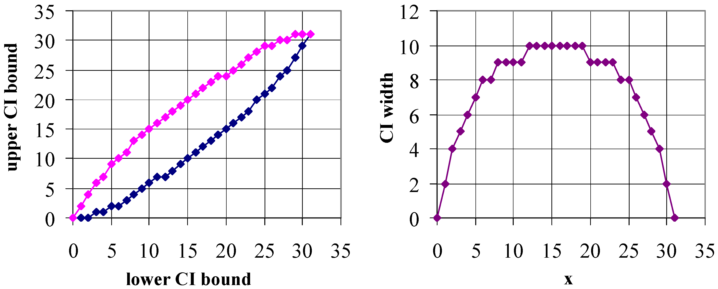
As can be observed from the above figures, the confidence interval boundaries of Algorithms 1 and 2 are monotonic, while those of Algorithm 3 are not (see Figure 9 left). Nevertheless, the confidence interval itself is monotonic and symmetric from the middle (see Figure 9 right). In contrast, the (supposed) optimum confidence interval built on monotonies (see Figure 6 right) is symmetric but not monotonic relative to the center.

Comparing Figure 6 with Figure 8 and Figure 10 with Figure 12 it can be observed that the monotonic increase of the boundaries leads to erroneous confidence intervals in the middle (Figure 6 vs. Figure 8), and is departing from the optimal (see SE($ϵ$) for Figure 10 vs. Figure 12).

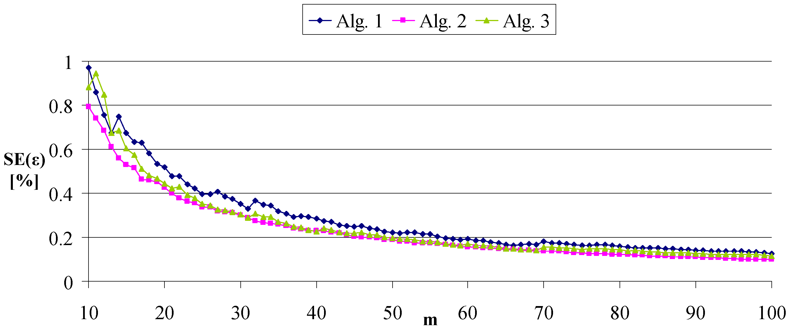
The standard error of the estimate (SE) as function of the sample size for samples from 10 to 100 shows the expected behavior of increasing precision with sample size (Figure 14).

In retrospect, the improvement proposed by Algorithm 3 vs. Algorithms 1 and 2 seems insignificant (see SE in Figure 12 vs. in Figure 13) in relation to the effects—the intervals, even if they are of monotonous width relative to the middle (Figure 8 right and Figure 9 right), and are still in a zig-zag form (see Figure 8 left and Figure 9 left).

Once we have the confidence interval for a binomially distributed variable (such as the ones proposed by the Algorithm 1 to Algorithm 3) we can derive the confidence interval for the proportion (Equation 11).

$$\begin{array}{c}\hfill \mathrm{If}[x_1,x_2]\mathrm{confidence}\mathrm{interval}\mathrm{for}x\mathrm{successes}\mathrm{from}m\mathrm{trials}\\ \hfill \mathrm{Then}\left[\frac{x_1}{m},\frac{x_2}{m}\right]\mathrm{confidence}\mathrm{interval}\mathrm{for}\frac{x}{m}\end{array}$$

(11)

Roughly the same calculations are involved when the binomial distribution (Equation (3)) is replaced with multinomial distribution (Equation (12)) thus permitting the usual factorial analysis [31] to be enriched with statistical significance.

$$f_{\mathrm{M}}(u_1,\dots ,u_k;x_1,\dots ,x_k)\leftarrow \frac{{\prod }_{i=1}^k{x}_i^{u_i}}{{\prod }_{i=1}^k{u}_i!}\frac{m!}{m^m};m\leftarrow \sum _{i=1}^k{u}_i=\sum _{i=1}^k{x}_i$$

(12)

The multinomial distribution proportion is a generalization from the binomial distribution proportion (Equation (12); when $k\leftarrow 2$ Equation (12) becomes Equation (3). Further research is required to adapt the procedures for binomial distributed samples confidence intervals calculation for multinomial distributed variables and proportions.

Since Poisson distribution can be applied to systems with a large number of possible events, each of which is rare, a future work is to adapt the approach for it.

6. Conclusions

A strategy to provide exact confidence intervals for binomial distributed variables is elaborated. Three algorithms for calculation of three alternate confidence intervals are given with examples. All proposed alternatives provide antisymmetrical confidence intervals with symmetrical true errors improving the classical asymptotic method.

References

1. Ialongo, C. Confidence interval for quantiles and percentiles. Biochem. Med. 2019, 29, 010101. [Google Scholar] [CrossRef]
2. Jäntschi, L.; Bolboacă, S.-D. Performances of Shannon’s Entropy Statistic in Assessment of Distribution of Data. Ovidius Univ. Ann. Chem. 2017, 28, 30. [Google Scholar] [CrossRef] [Green Version]
3. Jäntschi, L. A test detecting the outliers for continuous distributions based on the cumulative distribution function of the data being tested. Symmetry 2019, 11, 835. [Google Scholar] [CrossRef] [Green Version]
4. Jäntschi, L. Detecting extreme values with order statistics in samples from continuous distributions. Mathematics 2020, 8, 216. [Google Scholar] [CrossRef] [Green Version]
5. Ruggles, R.; Brodie, H. An Empirical Approach to Economic Intelligence in World War II. J. Am. Stat. Assoc. 1947, 42, 72. [Google Scholar] [CrossRef]
6. Carter, E.-M.; Potts, H.-W.-W. Predicting length of stay from an electronic patient record system: A primary total knee replacement example. BMC Med. Inform. Decis. Mak. 2014, 14, 26. [Google Scholar] [CrossRef] [Green Version]
7. Jäntschi, L. Distribution fitting 16. How many colors are actually in the field? Buasvmcn. Hortic. 2012, 69, 184. [Google Scholar]
8. Fisher, R.A. The relation between the number of species and the number of individuals in a random sample of an animal population. Part 3. A Theoretical distribution for the apparent abundance of different species. J. Anim. Ecol. 1943, 12, 54. [Google Scholar] [CrossRef]
9. Devaurs, D.A.; Gras, R. Species abundance patterns in an ecosystem simulation studied through Fisher’s logseries. Simul. Model. Pract. Theor. 2010, 18, 100–123. [Google Scholar] [CrossRef] [Green Version]
10. Frigyik, B.A.; Kapila, A.; Gupta, M.R. Introduction to the Dirichlet Distribution and Related Processes: UWEE Technical Report UWEETR-2010-0006; University of Washington: Seattle, WA, USA, 2010; pp. 18–25. [Google Scholar]
11. Dümbgen, L.; Samworth, R.J.; Wellner, J.A. Bounding distributional errors via density ratios. Bernoulli 2021, 27, 818–852. [Google Scholar] [CrossRef]
12. Bolboacă, S.-D.; Achimaş-Cadariu, B.-A. Binomial Distribution Sample Confidence Intervals Estimation 2. Proportion-like Medical Key Parameters. Leonardo Electron. J. Pract. Technol. 2003, 3, 75. [Google Scholar]
13. Newcombe, R.-G. Two–sided confidence intervals for the single proportion: Comparison of seven methods. Stat. Med. 1998, 17, 857. [Google Scholar] [CrossRef]
14. Pires, A.-M.; Amado, C. Interval estimators for a binomial proportion: Comparison of twenty methods. REVSTAT Stat. J. 2008, 6, 165. [Google Scholar]
15. Clopper, C.; Pearson, E.-S. The use of confidence or fiducial limits illustrated in the case of the binomial. Biometrika 1934, 26, 404. [Google Scholar] [CrossRef]
16. Sterne, T.E. Some Remarks on Confidence or Fiducial Limits. Biometrika 1954, 41, 275. [Google Scholar]
17. Blyth, C.R.; Still, H.A. Binomial confidence intervals. J. Am. Stat. Assoc. 1983, 78, 108. [Google Scholar] [CrossRef]
18. Casella, G. Refining Binomial Confidence Intervals. Can. J. Stat. 1986, 14, 113. [Google Scholar] [CrossRef] [Green Version]
19. Blaker, H. Confidence curves and improved exact confidence intervals for discrete distributions. Can. J. Stat. 2000, 28, 783. [Google Scholar] [CrossRef] [Green Version]
20. Bolboacă, S.-D.; Jäntschi, L. Optimized confidence intervals for binomial distributed samples. Int. J. Pure Appl. Math. 2008, 47, 1. [Google Scholar]
21. Jäntschi, L. Formulas, Algorithms and Examples for Binomial Distributed Data Confidence Interval Calculation: Excess Risk, Relative Risk and Odds Ratio. Mathematics 2021, 9, 2506. [Google Scholar] [CrossRef]
22. Sprott, D.A. What Is Optimality in Scientific Inference? Lect. Notes Monog. Ser. 2004, 44, 133–152. [Google Scholar]
23. Crow, E.L. Confidence Intervals for a Proportion. Biometrika 1956, 43, 423. [Google Scholar] [CrossRef]
24. Wang, W. Smallest confidence intervals for one binomial proportion. J. Stat. Plan. Inference 2006, 136, 4293. [Google Scholar] [CrossRef]
25. Eisenstein, J.; Chang, D.I. Case study: Improving population and individual health through health system transformation in Washington state. NAM Perspectives. Nat. Acad. Med. 2017, 4, 201704e. [Google Scholar] [CrossRef]
26. Brown, L.-D.; Cai, T.-T.; DasGupta, A. Interval Estimation for a Binomial Proportion. Stat. Sci. 2001, 16, 101. [Google Scholar] [CrossRef]
27. Agresti, A.; Coull, B.-A. Approximate is Better than “Exact” for Interval Estimation of Binomial Proportions. Am. Stat. 1998, 52, 119–126. [Google Scholar]
28. Bayes, T. An Essay Towards Solving a Problem in the Doctrine of Chances. Philos. Trans. R. Soc. Lond. 1763, 50, 370. [Google Scholar] [CrossRef]
29. Fienberg, S.-E. When Did Bayesian Inference Become “Bayesian”? Bayesian Anal. 2006, 1, 1. [Google Scholar] [CrossRef]
30. Vasil’ev, V.; Vasilyeva, M. An Accurate Approximation of the Two-Phase Stefan Problem with Coefficient Smoothing. Mathematics 2020, 8, 1924. [Google Scholar] [CrossRef]
31. Jäntschi, L.; Bálint, D.; Pruteanu, L.-L.; Bolboacă, S.-D. Elemental factorial study on one–cage pentagonal faces nanostructure congeners. Mater. Discov. 2016, 5, 14. [Google Scholar] [CrossRef]
Figure 1. Actual non-coverage probability ( α ^ , in %) as function of the binomial random variable (x) for the asymptotic interval.
Symmetry 14 01104 g001
Figure 2. Actual non-coverage probability ( α ^ , in %) as function of the binomial random variable (x) for the first “exact method” proposed (see below).
Symmetry 14 01104 g002
Figure 3. Actual non-coverage probability ( α ^ , in %) as function of the binomial random variable (x) for the second “exact method” proposed (see below).
Symmetry 14 01104 g003
Figure 4. Actual non-coverage probability ( α ^ , in %) as function of the binomial random variable (x) for the third “exact method” proposed (see below).
Symmetry 14 01104 g004
Figure 5. Lower and upper bound of four alternatives to construct the CI: Normal (Equation (5)) and the three proposed algorithms (Algorithms 1–3) when m = 10 , x = 0 , 1 , , 10 and α = 0.05 .
Symmetry 14 01104 g005
Figure 6. Optimum CIs when monotony rule is fully enacted for m = 31 and α = 0.05 (bounds in the left hand image and width in the right hand image).
Symmetry 14 01104 g006
Figure 7. Algorithm 1 CIs for m = 31 and α = 0.05 (bounds in the left hand image and width in the right hand image).
Symmetry 14 01104 g007
Figure 8. Algorithm 2 CIs for m = 31 and α = 0.05 (bounds in the left hand image and width in the right hand image).
Symmetry 14 01104 g008
Figure 9. Algorithm 3 CIs for m = 31 and α = 0.05 (bounds in the left hand image and width in the right hand image).
Symmetry 14 01104 g009
Figure 10. Optimum CIs when monotony rule is fully enacted: α ^ (in %) when α = 5% is the imposed level (m = 31; x = 0, 1, …, m; CI in Figure 6; α ^ is probably the smoothest one, SE( ϵ ) = 0.301).
Symmetry 14 01104 g010
Figure 11. Algorithm 1 CIs: α ^ (in %) when α = 5% is the imposed level (m = 31; x = 0, 1, …, m; α ^ α for all x = 0, 1, …, m; SE( ϵ ) = 0.331).
Symmetry 14 01104 g011
Figure 12. Algorithm 2 CIs: α ^ (in %) when α = 5% is the imposed level (m = 31; x = 0, 1, …, m; α ^ better than the one from Figure 10, SE( ϵ ) = 0.288).
Symmetry 14 01104 g012
Figure 13. Algorithm 3 CIs: α ^ (in %) when α = 5% is the imposed level (m = 31; x = 0, 1, …, m; α ^ α for all x = 0, 1, …, m; α ^ is better than the one from Figure 10, SE( ϵ ) = 0.287).
Symmetry 14 01104 g013
Figure 14. Standard error of α ^ (in %) for CIs from Algorithms 1–3, when α = 5% is the imposed level (m ranges from 10 to 100).
Symmetry 14 01104 g014