Visualising Departures from Symmetry and Bowker’s X² Statistic

Abstract

Sometimes, the same categorical variable is studied over different time periods or across different cohorts at the same time. One may consider, for example, a study of voting behaviour of different age groups across different elections, or the study of the same variable exposed to a child and a parent. For such studies, it is interesting to investigate how similar, or different, the variable is between the two time points or cohorts and so a study of the departure from symmetry of the variable is important. In this paper, we present a method of visualising any departures from symmetry using correspondence analysis. Typically, correspondence analysis uses Pearson’s chi-squared statistic as the foundation for all of its numerical and visual features. In the case of studying the symmetry of a variable, Bowker’s chi-squared statistic, presented in 1948, provides a simple numerical means of assessing symmetry. Therefore, this paper shall discuss how a correspondence analysis can be performed to study the symmetry (or lack thereof) of a categorical variable when Bowker’s statistic is considered. The technique presented here provides an extension to the approach developed by Michael Greenacre in 2000.

1. Introduction

Studying the departure from symmetry between categorical variables that are cross-classified to form a contingency table has been a topic of much discussion over the past few decades. There is wealth of literature that is now available that examines the measuring, modelling and application of symmetric categorical variables including, but not confined to, the contributions of Agresti [1] (Section 10.4), Anderson [2] (Section 10.2), Bove [3], De Falguerolles and van der Heijden [4], Iki, Yamamoto and Tomizawa [5], Tomizawa [6], Yamamoto [7] and Yamamoto, Shimada and Tomizawa [8]. Most recently, Arellano-Valle, Contreras-Reyes and Stehlik [9] and Nishisato [10] provides a wide ranging discussion on symmetry from the perspective of quantification theory. Such techniques are generally applied to an $S\times S$ contingency table, denoted here by $\mathbf{N}$, where a categorical variable may be examined over, for example, two time periods or between two cohorts. When interest is on assessing departures from complete or perfect symmetry in $\mathbf{N}$, further information on the symmetric (or lack thereof) nature of the variables may be gained by partitioning $\mathbf{N}$ so that

$$\mathbf{N}=\mathbf{Y}+\mathbf{K}=\frac{1}{2}\left(\mathbf{N}+{\mathbf{N}}^T\right)+\frac{1}{2}\left(\mathbf{N}-{\mathbf{N}}^T\right)$$

(1)

where $\mathbf{Y}$ is the matrix reflecting the symmetric part of $\mathbf{N}$ while $\mathbf{K}$ is the skew-symmetric part of the matrix. This partition was considered by Bove [3], Constantine and Gower [11] (Section 3), Gower [12] and Greenacre [13] for visualising row and column categories that deviate from the null hypothesis of perfect symmetry. Greenacre [13] shows how (1) can be used when performing a correspondence analysis on $\mathbf{N}$. His approach yields two visual summaries—one reflecting the symmetric structure (by performing a correspondence analysis on $\mathbf{Y}$) and another that visualises that part of the structure that is not symmetric (through a correspondence analysis of $\mathbf{K}$).

In this paper, we also consider how one may perform a correspondence analysis on a contingency table formed from the cross-classification of symmetric variables. Our strategy is different, but not completely independent, to that of Greenacre’s [13] method. The similarities of our approach and those of Greenacre [13] include basing our analysis on a weighted version of $\mathbf{K}$ that yields pairs of equivalent principal inertia values. However, the key difference of our technique when compared with Greenacre’s [13] is that we show how the approach outlined below can be performed when the underlying measure of the departure from perfect symmetry is Bowker’s [14] chi-squared statistic. By doing so, we show, for example, that there exists a link between the principal coordinates and singular values that are obtained and Bowker’s statistic.

For our discussion, this paper consists of seven further sections. Section 2 provides an overview of correspondence analysis which is typically used for visually exploring departures from complete independence between the categorical variables. In this section, we describe the application of singular value decomposition (SVD) to a transformation of a standard two-way contingency table, we define the principal coordinates needed to construct the visual summary and describe other key features. We then turn our attention to presenting an overview of the test of symmetry between the two categorical variables and the role that Bowker’s chi-squared statistic plays in such a test; see Section 3. Section 4 then shows how Bowker’s statistic can be used as the core global measure for assessing the variable’s departure from symmetry when providing a visual summary of such sources of departure using correspondence analysis. Section 5 illustrates some features of correspondence analysis when applied to Bowker’s statistic. Two examples are then presented that demonstrate the applicability of the technique. Section 6 applies this method of correspondence analysis to an artificially constructed $4\times 4$ contingency table that exhibits perfect symmetry when a constant $C=0$ is added to the $\left(2,1\right)$th cell frequency. Changes in C then provide a means of visualising the extent to which the rows and columns deviate from what is expected when the two variables are perfectly symmetric. Our second example, studied in Section 7, considers the data presented in Grover and Srinivasan [15], which looks at differences in the purchase of five brands of decaffeinated coffee across two time periods. Section 8 provides some final comments on the technique, including possible extensions and emendations that may be considered for future research. Three appendices are also included. The first two appendices derive the singular values for a contingency table of size $2\times 2$ and $3\times 3$ (both of which always yields an optimal display that consists of two dimensions). The third appendix provides a description of the R function bowkerca.exe() that performs the necessary calculations of the approach described in this paper.

2. On the Classical Approach

Before we outline our approach to the correspondence analysis of a contingency table using Bowker’s chi-squared statistic it is worth providing a broad overview of the classical technique; one may also consider, for example, Beh and Lombardo [16] for a detailed historical, methodological, practical and computational discussion of a range of correspondence analysis methods. To do so, we consider a contingency table, $\mathbf{N}$ of size $I\times J$ so that there are I row categories and J column categories. The $\left(i,j\right)$th cell frequency of $\mathbf{N}$ is denoted by $n_{ij}$ so that the total sample size is $n={\sum }_{i=1}^I{\sum }_{j=1}^J{n}_{ij}$. Denote the matrix of relative proportions by $\mathbf{P}$ where the $\left(i,j\right)$th value is $p_{ij}=n_{ij}/n$ so that the sum of these proportions across all $IJ$ cells of the table is 1. We also define the ith row marginal proportion by $p_{i•}={\sum }_{j=1}^J{p}_{ij}$ so that it is the ith element of the vector $\mathbf{r}$ and the $\left(i,i\right)$th element of the diagonal matrix ${\mathbf{D}}_R$. Similarly, the jth column marginal proportion is denoted by $p_{•j}={\sum }_{i=1}^I{p}_{ij}$, so that it is the jth element of the vector $\mathbf{c}$ and the $\left(j,j\right)$th element of the diagonal matrix ${\mathbf{D}}_C$.

To test whether the observed set of proportions, $p_{ij}$, differs from what is expected under some model with an expected value of ${\widehat{p}}_{ij}$, then Pearson’s chi-squared statistic for such a test takes the form

$$X^2=n\sum _{i=1}^S\sum _{j=1}^S\frac{{\left(p_{ij}-{\widehat{p}}_{ij}\right)}^2}{{\widehat{p}}_{ij}}.$$

(2)

For example, under the hypothesis of complete independence ${\widehat{p}}_{ij}=p_{i•}{p}_{•j}$ so that (2) becomes

$$X_I^2=n\sum _{i=1}^I\sum _{j=1}^J{r}_{ij}^2$$

(3)

where

$$r_{ij}=\frac{p_{ij}-p_{i•}{p}_{•j}}{\sqrt{p_{i•}{p}_{•j}}}$$

is the $\left(i,j\right)$th standardised (Pearson) residual and $X_I^2$ is a chi-squared random variable with $\left(I-1\right)\left(J-1\right)$ degrees of freedom. If there is a statistically significant association between the row and column variables this association can be visualised using correspondence analysis. This is achieved by first performing a SVD on the matrix of standardised residuals, such that

$${\mathbf{D}}_R^{-1/2}\left(\mathbf{P}-\mathbf{r}{\mathbf{c}}^T\right){\mathbf{D}}_C^{-1/2}=\mathbf{A}{\mathbf{D}}_{\lambda }{\mathbf{B}}^T.$$

Here, $\mathbf{A}$ and $\mathbf{B}$ are the column matrices containing the left and right singular vectors, respectively, and are constrained such that ${\mathbf{A}}^T\mathbf{A}={\mathbf{I}}_M$ and ${\mathbf{B}}^T\mathbf{B}={\mathbf{I}}_M$, where $M=min\left(I,J\right)-1$; here ${\mathbf{I}}_M$ is an $M\times M$ identity matrix. The $\left(m,m\right)$th element of the diagonal matrix ${\mathbf{D}}_{\lambda }$ is the mth singular value and these values arranged in descending order so that $1>{\lambda }_1>\dots >{\lambda }_M>0$.

A visual depiction of the association between the row and column variables can be made by simultaneously projecting the row principal coordinates and the column principal coordinates onto the same low-dimensional space which optimally consists of M dimensions; such a display is commonly referred to as a correspondence plot and typically consists of the first two dimensions (for ease of visualisation). The matrix of row and column principal coordinates are defined by

$$\begin{array}{ccc}\hfill \mathbf{F}& =& {\mathbf{D}}_R^{-1/2}\mathbf{A}{\mathbf{D}}_{\lambda }\hfill \\ \hfill \mathbf{G}& =& {\mathbf{D}}_C^{-1/2}\mathbf{B}{\mathbf{D}}_{\lambda }\hfill \end{array}$$

respectively.

Since (3) shows that Pearson’s chi-squared statistic is linearly related to the sample size, n, correspondence analysis uses $X^2/n$ as the measure of association which is termed the total inertia of the contingency table. This measure is directly related to the principal coordinates and singular values, such that

$$\begin{array}{ccc}\hfill \frac{X^2}{n}& =& \mathrm{trace}\left({\mathbf{D}}_{\lambda }^2\right)\hfill \\ & =& \mathrm{trace}\left({\mathbf{F}}^T{\mathbf{D}}_R\mathbf{F}\right)\hfill \\ & =& \mathrm{trace}\left({\mathbf{G}}^T{\mathbf{D}}_C\mathbf{G}\right).\hfill \end{array}$$

Therefore, points located at a great distance from the origin provide a visual indication of the importance that a category plays in the association structure of the variables, while the origin is the position of all of the row and column principal coordinates if there is complete independence between the variables.

We shall not provide a comprehensive account of all of the features, and related methods, of correspondence analysis. Instead, the interested reader is directed to Beh and Lombardo [16], for example, for more information.

3. On Studying the Symmetry of a Categorical Variable

Suppose we now wish to study the departure from complete symmetry of two categorical variables that share a similar structure. Let S be the number of categories contained in this variable so that the contingency table is now of size $S\times S$. Then, a test of symmetry of the variable may be undertaken by defining the null hypothesis by

$$H_0:p_{ij}=p_{ji};\forall i,j.$$

Sometimes, a study of symmetry in a contingency table may be undertaken by assessing the marginal homogeneity of the table where the null hypothesis is

$$H_0:p_{i•}=p_{•j};\forall i,j$$

but we shall say very little on this issue in the following sections.

When assessing whether there is any evidence of symmetry between the row and column variable of a contingency table, the most appropriate choice of ${\widehat{p}}_{ij}$ is

$${\widehat{p}}_{ij}=\frac{p_{ij}+p_{ji}}{2};$$

(4)

see, for example, Agresti [1] (p. 424) and Anderson [2] (p. 321). Substituting (4) into (2), and denoting the resulting statistic by $X_S^2$, yields

$$\begin{array}{ccc}\hfill X_S^2& =& \frac{n}{2}{\displaystyle \sum _{i=1}^S}{\displaystyle \sum _{j=1}^S}\frac{{\left(p_{ij}-p_{ji}\right)}^2}{p_{ij}+p_{ji}}\hfill \end{array}$$

(5)

$$\begin{array}{ccc}& =& n{\displaystyle \sum _{i>j}^S}\frac{{\left(p_{ij}-p_{ji}\right)}^2}{p_{ij}+p_{ji}}\hfill \end{array}$$

(6)

and is the chi-squared statistic derived by Bowker [14] for testing the symmetry between a row and column variable of a contingency table and has $S\left(S-1\right)/2$ degrees of freedom. When $S=2$ (6) simplifies to McNemar’s [17] statistic for testing the symmetry of two cross-classified dichotomous variables.

The simplicity of using (6) has gained wide appeal and was considered in the classic texts of Agresti [1] (p. 424), Bishop, Fienberg and Holland [18] (p. 283), Lancaster [19] (p. 236) and Plackett [20] (p. 59). However, Agresti [1] (p. 425) does point out that “it rarely fits well. When the marginal distributions differ substantially, it fits poorly”. The concern here about the poor fit when the margins of the contingency table differ substantially assumes that one is also interested in testing the independence between the categories. This is because when one assumes independence in the context of symmetry (4) becomes

$${\widehat{p}}_{ij}=\frac{p_{i•}{p}_{•j}+p_{j•}{p}_{•i}}{2}$$

and requires that $p_{i•}=p_{•i}$ for all $i=1,2,\dots ,S$, which we need not impose for testing symmetry. Perhaps what helps to clarify this point is that Lancaster [19] (p. 237) says that “more difficulties arise if…it is desired to test the homogeneity of the margins since $p_{ij}$ may not be equal to $p_{i•}{p}_{•j}$”. Since we are not concerned with testing for marginal homogeneity in this paper this “difficulty” is of no concern to us. We are also not greatly concerned with the inferential aspects of the statistic since (6) is used as a numerical basis on which correspondence analysis lies; in doing so, we are assuming, or have a priori tested and confirmed, that there is a departure from symmetry and we wish only to visualise the potential sources of this departure.

One may also consider the log-likelihood ratio statistic

$$\begin{array}{ccc}\hfill G_S^2& =& 2n{\displaystyle \sum _{i=1}^I}{\displaystyle \sum _{j=1}^I}{p}_{ij}ln\left(\frac{p_{ij}}{{\widehat{p}}_{ij}}\right)\hfill \\ & =& 2n{\displaystyle \sum _{i\ne j}}{p}_{ij}ln\left(\frac{2p_{ij}}{p_{ij}+p_{ji}}\right)\hfill \end{array}$$

as an alternative to $X_S^2$; see Bishop, Fienberg and Holland [18] (p. 283). We shall not discuss how this statistic can be used for studying departures from symmetry using correspondence analysis. However, the log-likelihood statistic, like Pearson’s statistic of (3), is a special case of the Cressie–Read family of divergence statistics [21] and Beh and Lombardo [22] provide an overview of how one may perform correspondence analysis using this divergence statistic. Future research can certainly be undertaken to study the role of $G_S^2$ in correspondence analysis when studying the symmetry of a categorical variable.

4. On Bowker’s Residuals and Departures from Symmetry

Let $\mathbf{S}$ be the matrix of the Bowker residuals where the $\left(i,j\right)$th element is

$$s_{ij}=\frac{1}{\sqrt{2}}\frac{p_{ij}-p_{ji}}{\sqrt{p_{ij}+p_{ji}}}$$

(7)

so that Bowker’s statistic, $X_S^2$ defined by (5), can be expressed as

$$\begin{array}{ccc}\hfill X_S^2& =& n{\displaystyle \sum _{i=1}^S}{\displaystyle \sum _{j=1}^S}{s}_{ij}^2\hfill \\ & =& n\mathrm{trace}\left({\mathbf{S}}^T\mathbf{S}\right)\hfill \\ & =& n\mathrm{trace}\left(\mathbf{S}{\mathbf{S}}^T\right).\hfill \end{array}$$

(8)

A feature of the matrix $\mathbf{S}$ (and $\mathbf{K}$ in (1)) is that it is an anti-symmetric, or skew-symmetric, matrix so that ${\mathbf{S}}^T=-\mathbf{S}$. Therefore, the left and right singular vectors, and the singular values, of the matrix of the Bowker residuals, $\mathbf{S}$, can be obtained from the eigen-decomposition of ${\mathbf{S}}^T\mathbf{S}$ or, equivalently, of $-{\mathbf{S}}^2$. If S is odd then there will always be a zero eigen-value and $S-1$ positive eigen-values; see Ward and Gray [23] and Gower [12] (p. 113). Ward and Gray [23] also present an algorithm that can perform the necessary eigen-decomposition and in Appendix A and Appendix B we provide a derivation that leads to closed-form solutions of the eigen-values of a $2\times 2$ and $3\times 3$ matrix of the Bowker residuals. Constantine and Gower [11] note that, since ${\mathbf{S}}^T\mathbf{S}=-{\mathbf{S}}^2$, there will be pairs of identical eigen-values. This is a feature that is also demonstrated in the appendices and described in Section 6 and Section 7.

Suppose we denote the $\left(i,j\right)$th element of $\mathbf{Y}$ and $\mathbf{K}$ from (1) by $y_{ij}$ and $k_{ij}$, respectively. Then, the $\left(i,j\right)$th Bowker residual—see (7)—can be alternatively expressed as

$$s_{ij}=\frac{1}{2}\left(p_{ij}-p_{ji}\right)÷\sqrt{\frac{1}{2}\left(p_{ij}+p_{ji}\right)}=\frac{k_{ij}}{\sqrt{y_{ij}}}.$$

(9)

Therefore, Bowker’s residuals do assess for each cell of the contingency table where departures from symmetry exist but they do so relative to the amount of symmetry that exists between the two variables. This is in contrast to Greenacre’s [13] approach which considers a residual where $k_{ij}$ is divided by the mean of the row and column marginal proportions; for the ith such proportion this is $\left(p_{i•}+p_{•i}\right)/2$ for $i=1,2,\dots ,S$.

In addition, since the numerator of $\mathbf{S}$ can be expressed in terms of $\mathbf{K}$ this ensures that Bowker’s residuals are centred at zero under perfect symmetry (a property shared with Greenacre’s [13] approach). This is important since it means that the principal coordinates that we derive in Section 5.3 are centred at the origin of the optimal correspondence plot.

5. Correspondence Analysis and Bowker’s Statistic

5.1. On the SVD of the Matrix of the Bowker Residuals

Visually detecting departures from symmetry can be undertaken using correspondence analysis. This can be achieved by first applying a SVD to $\mathbf{S}$ such that

$$\mathbf{S}=\mathbf{A}{\mathbf{D}}_{\lambda }{\mathbf{B}}^T.$$

(10)

Here, the $S\times M$ column matrix $\mathbf{A}$ contains the left singular vectors of $\mathbf{S}$ and have the property ${\mathbf{A}}^T\mathbf{A}={\mathbf{I}}_M$. Similarly, $\mathbf{B}$ is a $S\times M$ column matrix of the right singular vectors such that ${\mathbf{B}}^T\mathbf{B}={\mathbf{I}}_M$ of $\mathbf{S}$. While $M=min\left(S,S\right)-1=S-1$ for the classical approach to correspondence analysis, this is not the case for the analysis of the matrix of the Bowker residuals. Since $\mathbf{S}$ is a skew-symmetric matrix there will be S singular values when S is even and $S-1$ such values when S is odd. Therefore,

$$M=\left\{\begin{array}{c}S,\mathrm{if}S\mathrm{is}\mathrm{even}\hfill \\ S-1,\mathrm{if}S\mathrm{is}\mathrm{odd}\hfill \end{array}\right..$$

Gower [12] showed that since $\mathbf{S}$ is skew-symmetric then the SVD of the matrix, (10), is equivalent to

$$\mathbf{S}=\mathbf{A}{\mathbf{D}}_{\lambda }{\mathbf{J}}_M{\mathbf{A}}^T$$

(11)

so that

$$\mathbf{B}=\mathbf{A}{\mathbf{J}}_M^T.$$

(12)

Here ${\mathbf{J}}_M$ is a $M\times M$ block diagonal and orthogonal skew-symmetric matrix so that

$${\mathbf{J}}_M^T{\mathbf{J}}_M={\mathbf{J}}_M{\mathbf{J}}_M^T={\mathbf{I}}_M$$

(13)

where ${\mathbf{I}}_M$ is an $M\times M$ identity matrix. When $M=2$,

$${\mathbf{J}}_2=\left(\begin{array}{cc}0& 1\\ -1& 0\end{array}\right)$$

while

$${\mathbf{J}}_4=\left(\begin{array}{cccc}0& 1& 0& 0\\ -1& 0& 0& 0\\ 0& 0& 0& 1\\ 0& 0& -1& 0\end{array}\right).$$

If S is odd then the $\left(S,S\right)$th element is 1 and the rest of its row/column consists of zeros so that  

$${\mathbf{J}}_S=\left(\begin{array}{cc}{\mathbf{J}}_{S-1}& {\mathbf{0}}_{S-1}^T\\ {\mathbf{0}}_{S-1}& 1\end{array}\right)$$

where ${\mathbf{0}}_{S-1}$ is a zero vector of length $S-1$. For example,

$${\mathbf{J}}_3=\left(\begin{array}{ccc}0& 1& 0\\ -1& 0& 0\\ 0& 0& 1\end{array}\right).$$

The $M\times M$ diagonal matrix ${\mathbf{D}}_{\lambda }$ contains the singular values of $\mathbf{S}$ and are arranged in consecutive pairs of values so that $1>{\lambda }_1={\lambda }_2>{\lambda }_3={\lambda }_4>\dots \ge 0$. This feature will be discussed in the next section, but it is worth noting that the SVD presented in (11) makes use of the Murnaghan canonical form of $\mathbf{S}$; see Murnaghan and Wintner [24] and Paardekooper [25] for further information on this decomposition.

5.2. The Total Inertia

Quantifying the departure from symmetry can be undertaken by calculating the total inertia of $\mathbf{S}$ which is just Bowker’s statistic divided by the sample size, $X_S^2/n$. When $\mathbf{B}$, for example, is of full rank, then $\mathbf{B}{\mathbf{B}}^T={\mathbf{B}}^T\mathbf{B}$. Thus, using (8), the total inertia can be expressed as the sum-of-squares of the singular values such that

$$\begin{array}{ccc}\hfill {\varphi }_S^2& =& \frac{X_S^2}{n}\hfill \\ & =& \mathrm{trace}\left({\left(\mathbf{A}{\mathbf{D}}_{\lambda }{\mathbf{B}}^T\right)}^T\left(\mathbf{A}{\mathbf{D}}_{\lambda }{\mathbf{B}}^T\right)\right)\hfill \\ & =& \mathrm{trace}\left(\mathbf{B}{\mathbf{D}}_{\lambda }^2{\mathbf{B}}^T\right)\hfill \\ & =& \mathrm{trace}\left({\mathbf{D}}_{\lambda }^2\right).\hfill \end{array}$$

When visualising departures from symmetry, one may construct a correspondence plot consisting of at most M dimensions where the principal inertia (or weight) of the mth dimension is ${\lambda }_m^2$. Therefore, expressing the total inertia in terms of the matrix ${\mathbf{D}}_{\lambda }^2$ (or the elements ${\lambda }_m^2$) provides a means of determining, for each dimension, the percentage of the total departure from symmetry that exists between the row and column variables. Such a percentage is calculated by

$$100\times \frac{{\lambda }_m^2}{{\varphi }_S^2}.$$

Since ${\lambda }_1={\lambda }_2$ is the largest pair of singular values, the first and second dimensions visually provide the best (and an equivalent quality) depiction of any departure from symmetry that exists in $\mathbf{N}$. For example, when $S=5$, say, the first and second dimensions will always provide the same (and most) amount of information to the visual display, while the third and fourth dimensions will be equally weighted and display less of the departure. These four dimensions will provide an optimal display of the departure from symmetry since the fifth dimension will have a zero principal inertia value.

5.3. The Principal Coordinates

When calculating Bowker’s statistic, only the cell proportions $p_{ij}$ and $p_{ji}$ are used, not the marginal proportions; see (5) and equivalently (6). The cloud-of-points generated for the rows and columns can be obtained by aggregating these cell proportions across the row and column variables, yielding two spaces that have the same metric; this metric being $\widehat{\mathbf{D}}=\left({\mathbf{D}}_R+{\mathbf{D}}_C^T\right)/2$. Such a property is consistent, but slightly different, to the traditional approach to correspondence analysis which assesses departures from independence, not symmetry, and so assumes that the row space and column space have a metric based on the aggregation of $p_{ij}$ across the two variables. That is, the row space has the metric ${\mathbf{D}}_R$ while the column metric is ${\mathbf{D}}_C$. Thus, the metric $\widehat{\mathbf{D}}$ is the average of the row and column spaces and is consistent with the metric adopted by Greenacre [13].

To obtain a visual depiction of the departures from symmetry one may simultaneously plot the row and column principal coordinates which are defined in terms of the above matrices by

$$\begin{array}{ccc}\hfill \mathbf{F}& =& {\widehat{\mathbf{D}}}^{-1/2}\mathbf{A}{\mathbf{D}}_{\lambda }\hfill \end{array}$$

(14)

$$\begin{array}{ccc}\hfill \mathbf{G}& =& {\widehat{\mathbf{D}}}^{-1/2}\mathbf{B}{\mathbf{D}}_{\lambda }\hfill \end{array}$$

(15)

respectively.

5.4. On the Origin and Transition Formulae

The total inertia of the two-way contingency table can be expressed in terms of the principal coordinates defined by (14) and (15). For example, for the row coordinates,

$$\begin{array}{ccc}\hfill \mathrm{trace}\left({\mathbf{F}}^T\widehat{\mathbf{D}}\mathbf{F}\right)& =& \mathrm{trace}\left({\left({\widehat{\mathbf{D}}}^{-1/2}\mathbf{A}{\mathbf{D}}_{\lambda }\right)}^T\widehat{\mathbf{D}}\left({\widehat{\mathbf{D}}}^{-1/2}\mathbf{A}{\mathbf{D}}_{\lambda }\right)\right)\hfill \\ & =& \mathrm{trace}\left({\mathbf{D}}_{\lambda }^T{\mathbf{A}}^T\mathbf{A}{\mathbf{D}}_{\lambda }\right)\hfill \\ & =& \mathrm{trace}\left({\mathbf{D}}_{\lambda }^2\right)\hfill \\ & =& \frac{X_S^2}{n}.\hfill \end{array}$$

This shows that the origin coincides with the location of all row coordinates when there is perfect symmetry between variables of the contingency table. By following a similar derivation, it can also be shown that

$$\frac{X_S^2}{n}=\mathrm{trace}\left({\mathbf{G}}^T\widehat{\mathbf{D}}\mathbf{G}\right).$$

These expressions of the total inertia also show that points located far from the origin identify categories that deviate from what is expected if there was perfect symmetry.

Alternative expressions of the matrices of row and column principal coordinates can also be obtained. For example, suppose we consider (14). Then, by post-multiplying both sides by ${\mathbf{B}}^T$ and simplifying we get

$$\mathbf{F}={\widehat{\mathbf{D}}}^{-1/2}\mathbf{S}\mathbf{B}.$$

Thus, the $\left(i,m\right)$’th element of $\mathbf{F}$ is

$$\begin{array}{ccc}\hfill f_{im}& =& \frac{\sqrt{2}}{\sqrt{p_{i•}+p_{•i}}}{\displaystyle \sum _{j=1}^J}{s}_{ij}{b}_{jm}\hfill \\ & =& \frac{\sqrt{2}}{\sqrt{p_{i•}+p_{•i}}}{\displaystyle \sum _{j=1}^J}\frac{1}{\sqrt{2}}\frac{p_{ij}-p_{ji}}{\sqrt{p_{ij}+p_{ji}}}{b}_{jm}\hfill \\ & =& {\displaystyle \sum _{j=1}^J}\frac{p_{ij}-p_{ji}}{\sqrt{\left(p_{i•}+p_{•i}\right)\left(p_{ij}+p_{ji}\right)}}{b}_{jm}.\hfill \end{array}$$

Therefore, a principal coordinate will lie at the origin of the correspondence plot if there is perfect symmetry between the ith row and ith column; that is, when $p_{ij}=p_{ji}$ for all $j=1,2,\dots ,S$, thus verifying expressing the total inertia in terms of the matrix of row principal coordinates. Any departure from symmetry of the ith row from the ith column will result in the ith principal coordinate moving away from the origin. This implies that the ith column category will also move away from the origin but it will do so in a different direction from the row category. Such a feature can be verified by showing that the row and column principal coordinates are linked through the following transition formulae. By substituting (12) into (15) the matrix of column principal coordinates can be alternatively expressed as

$$\mathbf{G}={\widehat{\mathbf{D}}}^{-1/2}\mathbf{A}{\mathbf{J}}_M^T{\mathbf{D}}_{\lambda }={\widehat{\mathbf{D}}}^{-1/2}\mathbf{A}{\mathbf{D}}_{\lambda }{\mathbf{J}}_M^T.$$

Thus, the matrix of column principal coordinates can be expressed in terms of the matrix of row principal coordinates such that

$$\mathbf{G}=\mathbf{F}{\mathbf{J}}_M^T.$$

(16)

Similarly, post-multiplying both sides of (16) by ${\mathbf{J}}_M$ and using (13) leads to

$$\mathbf{F}=\mathbf{G}{\mathbf{J}}_M.$$

(17)

showing how the matrix of row principal coordinates can be expressed in terms of the matrix of column principal coordinates. Thus, for the ith row and column categories, $\left(f_{i1},f_{i2}\right)=\left(-g_{i2},g_{i1}\right)$ showing that departures from symmetry between these two categories will position their principal coordinates on opposite sides of the correspondence plot, unless there is perfect symmetry in which case both will lie at the origin.

5.5. Intra-Variable Distances

Suppose we are interested in the distance between the ith and $i^{\prime }$th row principal coordinates in a correspondence plot. It can be shown that the squared Euclidean distance between $f_{im}$ and $f_{i^{\prime }m}$ is

$$\begin{array}{ccc}\hfill d_I^2\left(i,i^{\prime }\right)& =& {\displaystyle \sum _{j=1}^S}{c}_{ij}{\left[\frac{p_{ij}+p_{i^{\prime }j}}{2}-\frac{p_{ji}+p_{j{i}^{\prime }}}{2}\right]}^2\hfill \end{array}$$

(18)

$$\begin{array}{ccc}& \hspace{1em}\hspace{1em}\hspace{1em} =& {\displaystyle \sum _{j=1}^S}{c}_{ij}{\left[\frac{p_{ij}-p_{ji}}{2}+\frac{p_{i^{\prime }j}-p_{j{i}^{\prime }}}{2}\right]}^2\hfill \end{array}$$

(19)

where  

$$c_{ij}=\frac{p_{•j}+p_{j•}}{\sqrt{\left(p_{ij}+p_{ji}\right)\left(p_{i^{\prime }j}+p_{j{i}^{\prime }}\right)}}$$

Thus, if $p_{ij}+p_{i^{\prime }j}=p_{ji}+p_{j{i}^{\prime }}$ or, equivalently, ${\widehat{p}}_{ij}={\widehat{p}}_{i^{\prime }j}$ for all $j=1,2,\dots ,S$ then the ith and $i^{\prime }$th row principal coordinates will be located in the same position in the optimal correspondence plot. Such a feature arises when the expected cell frequency (under perfect symmetry) is the same for the ith and $i^{\prime }$th rows. Alternatively, $f_{im}=f_{i^{\prime }m}$, for all $m=1,2,\dots ,S$ when $p_{ij}-p_{ji}=p_{i^{\prime }j}-p_{i{j}^{\prime }}$. This feature does not imply that there must be perfect symmetry between the ith and $i^{\prime }$th row categories, but it does arise when any departure from perfect symmetry is the same for these categories.

6. Example 1 Artificial Data

6.1. The Data

To examine how to perform a correspondence analysis on a contingency table using Bowker’s statistic (6), suppose we consider the artificial data presented in Table 1. Here, $C\ge 0$ in the $\left(2,1\right)$th cell is a non-negative integer ensuring that Table 1 maintains the features of a contingency table. For this table, Bowker’s statistic is

$$\begin{array}{ccc}\hfill X_S^2& =& {\displaystyle \sum _{i>j}^4}\frac{{\left(n_{ij}-n_{ji}\right)}^2}{n_{ij}+n_{ji}}\hfill \\ & =& \frac{{\left(n_{21}-n_{12}\right)}^2}{n_{21}+n_{12}}+\frac{{\left(n_{31}-n_{13}\right)}^2}{n_{31}+n_{13}}+\frac{{\left(n_{41}-n_{14}\right)}^2}{n_{41}+n_{14}}\hfill \\ & & +\frac{{\left(n_{32}-n_{23}\right)}^2}{n_{32}+n_{23}}+\frac{{\left(n_{42}-n_{24}\right)}^2}{n_{42}+n_{24}}+\frac{{\left(n_{43}-n_{34}\right)}^2}{n_{43}+n_{34}}\hfill \end{array}$$

(20)

$$\begin{array}{ccc}& =& \frac{C^2}{40+C}\hspace{1em}\hspace{1em}\hspace{1em}\hspace{1em}\hspace{1em}\hspace{1em}\hspace{1em}\hspace{1em}\hspace{1em}\hspace{1em}\hspace{1em}\hspace{1em}\hspace{1em}\hspace{1em}\hspace{1em} \hfill \end{array}$$

(21)

and is a chi-squared random variable with $4\times \left(4-1\right)/2=6$ degrees of freedom. Therefore, (21) shows that when $C=0$, Bowker’s chi-squared statistic is zero and Table 1 is perfectly symmetric.

Table 1. A near-symmetric artificial contingency table where C is a non-negative integer.

	C1	C2	C3	C4
R1	10	20	30	40
R2	20 + C	50	60	70
R3	30	60	20	40
R4	40	70	40	80

6.2. Preliminary Examination of the Departure from Symmetry

Departures from symmetry for Table 1 can be assessed by determining the minimum value of C so that $X_S^2>{\chi }_{\alpha }^2\left(6\right)$. That is, when

$$\frac{C^2}{40+C}>{\chi }_{\alpha }^2\left(6\right).$$

From this result, one may obtain the following quadratic equation (in terms of C)

$$C^2-{\chi }_{\alpha }^2\left(6\right)\times C-40{\chi }_{\alpha }^2\left(6\right)>0$$

which only has one valid solution

$$C=\frac{{\chi }_{\alpha }^2\left(6\right)+\sqrt{{\left({\chi }_{\alpha }^2\left(6\right)\right)}^2+160{\chi }_{\alpha }^2\left(6\right)}}{2}$$

that ensures that C is non-negative. For example, when testing symmetry using $\alpha =0.05$, ${\chi }_{0.05}^2\left(6\right)=12.59$ so that C must exceed 29.59 for the departure from symmetry to be statistically significant. For practical purposes, C must be an integer of at least 30 to ensure that the $\left(2,1\right)$th cell remains a positive integer. Hence, this cell frequency must exceed 50 for there to be a statistically significant lack of symmetry in Table 1. Thus, to demonstrate how the correspondence analysis technique described in Section 5 can be applied to Table 1 we shall be considering the following values of C; 50, 75, 100 and 150. These values of C give a Bowker statistic of 27.78, 48.91, 71.43 and 118.42, respectively, which all have a p-value that is less than 0.001.

6.3. Features of Correspondence Analysis & Symmetry

Interestingly, for Table 1, closed form expressions exist for many of the features that come from the correspondence analysis of contingency table when examining departures from symmetry. To show this, suppose consider again the matrix of the Bowker residuals, $\mathbf{S}$. For Table 1, this matrix is

$$\mathbf{S}=\left(\begin{array}{cccc}0& -\frac{C}{\sqrt{2n\left(40+C\right)}}& 0& 0\\ \frac{C}{\sqrt{2n\left(40+C\right)}}& 0& 0& 0\\ 0& 0& 0& 0\\ 0& 0& 0& 0\end{array}\right).$$

The structure of this $4\times 4$ matrix is identical to a $2\times 2$ matrix when removing the vectors of zeros in the last two rows and columns of $\mathbf{S}$. In Appendix A we show that when $\mathbf{S}$ is of size $2\times 2$, then applying a SVD to it yields the singular values

$${\lambda }_1={\lambda }_2=\frac{C}{\sqrt{2n\left(40+C\right)}}\left(=s_{21}=-s_{12}\right)$$

(22)

thereby producing two non-trivial, and identical, singular values, and one zero singular value. Thus, the sum-of-squares of these singular values gives, for Table 1, a total inertia of

$${\varphi }_S^2={\lambda }_1^2+{\lambda }_2^2+{\lambda }_3^2=\frac{C^2}{n\left(40+C\right)}.$$

Note that this is equivalent to (21) divided by the sample size n. Since $n=680+C$ then the total inertia can be expressed in terms of C by

$${\varphi }_S^2\left(C\right)=\frac{C^2}{\left(680+C\right)\left(40+C\right)}$$

so that, for Table 1, $0\le {\varphi }_S^2\left(C\right)<1$ for $C\ge 0$.

Since there are only two, equivalent, non-trivial singular values, a two-dimensional correspondence plot will produce an optimal display of the departure from symmetry of Table 1 regardless of the value of C; the principal inertia of these two dimensions is ${\lambda }_1$ each. Thus, both dimensions of the optimal display will visually describe exactly half of the departure from symmetry which is quantified by ${\varphi }_S^2\left(C\right)$. Note that from (22) the first two singular values of $\mathbf{S}$ from Table 1 can be expressed as

$${\lambda }_1={\lambda }_2=\frac{C}{\sqrt{2\left(680+C\right)\left(40+C\right)}}$$

so that

$${\mathbf{D}}_{\lambda }=\frac{C}{\sqrt{2\left(680+C\right)\left(40+C\right)}}\left(\begin{array}{cc}1& 0\\ 0& 1\end{array}\right)$$

while, the first two non-trivial left and right singular vectors of $\mathbf{S}$ are

$$\mathbf{A}=\left(\begin{array}{cc}0& -1\\ -1& 0\\ 0& 0\\ 0& 0\end{array}\right)\mathrm{and}\mathbf{B}=\mathbf{A}{\mathbf{J}}_2^T=\left(\begin{array}{cc}-1& 0\\ 0& 1\\ 0& 0\\ 0& 0\end{array}\right),$$

respectively. The matrix $\widehat{\mathbf{D}}$ is

$$\widehat{\mathbf{D}}=\left(\begin{array}{cccc}\frac{200+C}{2\left(680+C\right)}& 0& 0& 0\\ 0& \frac{400+C}{2\left(680+C\right)}& 0& 0\\ 0& 0& \frac{150}{680+C}& 0\\ 0& 0& 0& \frac{230}{680+C}\end{array}\right)$$

so that

$${\widehat{\mathbf{D}}}^{-1/2}=\sqrt{680+C}\left(\begin{array}{cccc}\sqrt{\frac{2}{200+C}}& 0& 0& 0\\ 0& \sqrt{\frac{2}{400+C}}& 0& 0\\ 0& 0& \frac{1}{\sqrt{150}}& 0\\ 0& 0& 0& \frac{1}{\sqrt{230}}\end{array}\right).$$

Therefore, after some matrix manipulation, the matrix containing the row principal coordinates in the optimal two-dimensional correspondence plot can be expressed in terms of C and some constants (dependent on the cell frequencies of Table 1) such that

$$\mathbf{F}=\frac{C}{\sqrt{40+C}}\left(\begin{array}{cc}0& -\sqrt{\frac{1}{200+C}}\\ -\sqrt{\frac{1}{400+C}}& 0\\ 0& 0\\ 0& 0\end{array}\right).$$

(23)

By following a similar derivation, the matrix of column principal coordinates is

$$\mathbf{G}=\frac{C}{\sqrt{40+C}}\left(\begin{array}{cc}-\sqrt{\frac{1}{200+C}}& 0\\ 0& \sqrt{\frac{1}{400+C}}\\ 0& 0\\ 0& 0\end{array}\right).$$

(24)

Thus, (23) and (24) satisfy (16) and (17). The zeros in the third and fourth rows of $\mathbf{F}$ and $\mathbf{G}$ are because there is perfect symmetry between the third and fourth rows and columns of Table 1. So, the position of these points in the correspondence plot lie at the origin, irrespective of the choice of $C\ge 0$. When $C=0$, all principal coordinates for the row and column categories will lie at the origin since Table 1 exhibits perfect symmetry. Therefore, changes in C will lead to changes in the configuration depicted in the correspondence plot. For example, suppose $C=50$ so that, for Table 1, $n_{21}=70$. Then, the key features of the correspondence analysis when an examination of the departures from symmetry are being made using Bowker’s statistic can be simply calculated as follows:

$$\begin{array}{ccc}\hfill X_S^2& =& \frac{{50}^2}{40+50}=27.778\hfill \\ \hfill {\lambda }_1& =& {\lambda }_2=\frac{50}{\sqrt{2\left(680+50\right)\left(40+50\right)}}=0.138\hfill \\ \hfill f_{12}& =& -\frac{50}{\sqrt{\left(40+50\right)\times \left(200+50\right)}}=-0.333\hfill \\ \hfill f_{21}& =& -\frac{50}{\sqrt{\left(40+50\right)\left(400+50\right)}}=-0.248\hfill \\ \hfill g_{11}& =& -\frac{50}{\sqrt{\left(40+50\right)\left(200+50\right)}}=-0.333\hfill \\ \hfill g_{22}& =& \frac{50}{\sqrt{\left(40+50\right)\times \left(400+50\right)}}=0.248.\hfill \end{array}$$

A summary of these quantities for $C=50,75,100$ and 150 is given in Table 2.

Table 2. Select output from the correspondence analysis of Table 1 when studying departures from symmetry; $C=50,75,100$ and 150.

	C
Output	50	75	100	150
$X_S^2$	27.778	48.913	71.429	118.421
${\varphi }_S\left(C\right)$	0.038	0.065	0.092	0.143
${\lambda }_1$	0.138	0.180	0.214	0.267
$f_{12}$	−0.333	−0.422	−0.488	−0.582
$f_{21}$	−0.248	−0.321	−0.378	−0.464
$g_{11}$	−0.333	−0.422	−0.488	−0.582
$g_{22}$	0.248	0.321	0.378	0.464

Supplementing the numerical summaries that appear in Table 2 are the two-dimensional correspondence plots of Figure 1, Figure 2, Figure 3 and Figure 4. These figures, and their accompanying numerical features, can be obtained using the R function bowkerca.exe() that is described in Appendix C of this paper. Figure 1 shows such a plot for $C=50$, Figure 2 is the correspondence plot for $C=75$, Figure 3 is the plot for $C=100$ while the two-dimensional correspondence plot of Table 1 when $C=150$ is given by Figure 4. Based on the statements we made above, it should be of no surprise to see that these four plots show that its two dimensions visually describes exactly half of any departures from symmetry that exist between the variables of Table 1. Thus, each of the four correspondence plots is optimal in its visual depiction of such depatures; since ${\lambda }_1$ and ${\lambda }_2$ are equivalent for all values of C. These correspondence plots also show that C3, C4, R3 and R4 all share the same position at the origin since there is no departure from perfect symmetry for these categories. However, the position of R1, R2, C1 and C2 lie further from the origin as C increases since these categories increasingly deviate from perfect symmetry as C increases.

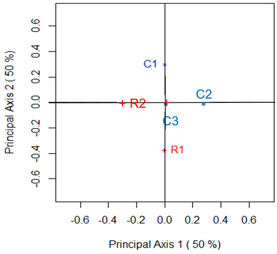
Figure 1. Correspondence plot that visually examines the departure from symmetry for Table 1; $C=50$.

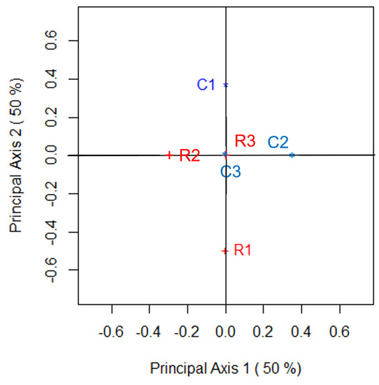
Figure 2. Correspondence plot that visually examines the departure from symmetry for Table 1; $C=75$.

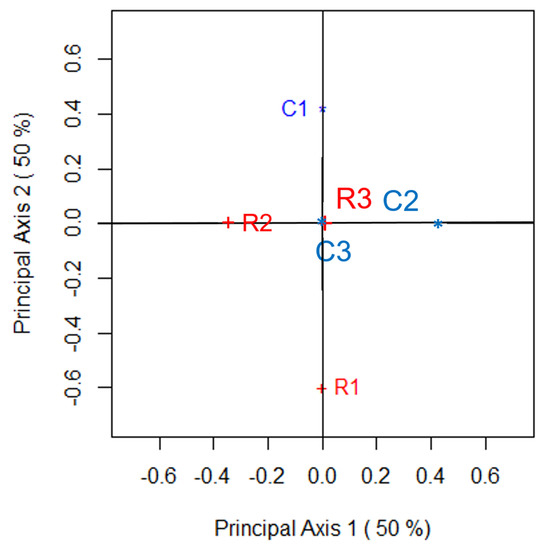
Figure 3. Correspondence plot that visually examines the departure from symmetry for Table 1; $C=100$.

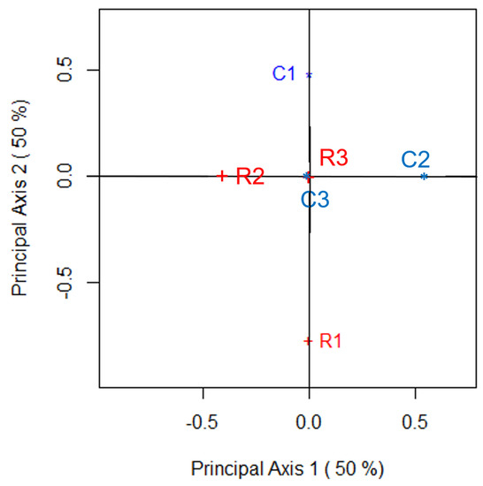
Figure 4. Correspondence plot that visually examines the departure from symmetry for Table 1; $C=150$.

While R1 and C2 are unaffected by changes in C, since symmetry is assessed by considering the difference between the $\left(2,1\right)$th and $\left(1,2\right)$th cell frequencies (or proportions), any departure from symmetry does impact their relative position from each other in the correspondence plot. This can be observed by noting that, along the second dimension,

$$\frac{f_{12}}{g_{22}}=-\sqrt{\frac{400+C}{200+C}}$$

is not independent of C. For $C>0$, $f_{12}$ and $g_{22}$ will always remain on opposite sides of the first dimension with $f_{12}$ being at most $\sqrt{2}$ units further away from the origin than $g_{22}$; as $C\to \infty$$f_{12}\to -g_{22}$.

We can gain an understanding of how the position of R1 and C1, say, in the optimal (two-dimensional) correspondence plot compare for $C>0$. Since $f_{12}<0$ and $g_{11}<0$, R1 will lie along the second dimension, while C1 will lie along the first dimension showing that their relative proximity from each other increases as C increases; note that we are not interpreting this row/column proximity in terms of a quantifiable distance measure. However, we can quantify how the relative position of R1 and C1 change by noting the ratio between these two coordinates is $f_{12}/g_{11}=1$ for all values of C. Therefore, R1 and C1 will move the same number of units away from the origin as C increases.

7. Example 2 on the Purchase of Decaffeinated Coffee

We now focus our attention on a $5\times 5$ contingency table considered by Agresti [26] (Table 8.5) whose original data came from Grover and Srinivasan [15]; see Table 3. For these data, 541 individuals were surveyed about their choice of purchase of five brands of decaffeinated coffee. Each of the participants were asked to record the brand they bought on their first and subsequent purchase. If every participant of the study bought the same brand of coffee on their first and second purchase then the contingency table would exhibit perfect symmetry. However, this was not the case, and so one may investigate where the departures from symmetry lie. In doing so, one can identify brands that had a similar purchasing pattern on the first and second purchase and those that did not.

Table 3. A simple $5\times 5$ table where we test for symmetry using CA.

	Second Purchase
First	High Pt	Taster’s	Sanka	Nescafé	Brim	Total
Purchase	(hp)	(ta)	(sa)	(ne)	(br)
High Point (HP)	93	17	44	7	10	171
Taster’s Choice (TC)	9	46	11	0	9	75
Sanka (SA)	17	11	155	9	12	204
Nescafé	6	4	9	15	2	36
Brim	10	4	12	2	27	55
Total	135	82	231	33	60	541

A test of symmetry can be performed and doing so yields a Bowker’s statistic of $20.265$. With $5\times \left(5-1\right)/2=10$ degrees of freedom, this statistic has a p-value of $0.027$ showing that there are departures from symmetry present in the data. An evaluation of where departures from symmetry lie in Table 3 can be made by observing the skew-symmetric matrix $\mathbf{S}$ which is

$$\mathbf{S}=\left(\begin{array}{ccccc}\hfill 0& \hfill 0.048& \hfill 0.105& \hfill 0.008& \hfill 0.000\\ \hfill -0.048& \hfill 0& \hfill 0& \hfill -0.061& \hfill 0.042\\ \hfill -0.105& \hfill 0& \hfill 0& \hfill 0& \hfill 0\\ \hfill -0.008& \hfill 0.061& \hfill 0& \hfill 0& \hfill 0\\ \hfill 0& \hfill -0.042& \hfill 0& \hfill 0& \hfill 0\end{array}\right).$$

Observing the relative size of the $s_{ij}$ values of this matrix shows that the greatest source of departure from symmetry appears to be for the coffee brand “High Point” while “Brim” is the coffee brand that deviates least from symmetry (although not perfectly). A visual depiction of the departures from symmetry that are present in Table 3 can be made by performing the correspondence analysis approach described above. Appendix C shows how the R function bowkerca.exe() can be used to perform this analysis on Table 3. This analysis gives the following two pairs of non-trivial singular values

$${\lambda }_1={\lambda }_2=0.1215\mathrm{and}{\lambda }_3={\lambda }_4=0.0641$$

so that their sum-of-squares gives the total inertia

$$\frac{X_S^2}{n}=0.{1215}^2+0.{1215}^2+0.{0641}^2+0.{0641}^2=0.0377.$$

A visual depiction of the departure from symmetry is given by Figure 5. The quality of this two-dimensional correspondence is excellent and accounts for

$$100\times \frac{0.{1215}^2+0.{1215}^2}{0.0377}=78.242\%$$

of the departure from symmetry that exists in Table 3. The row and column principal coordinates depicted in Figure 5 are

$$\mathbf{F}=\left(\begin{array}{cc}\hfill 0& \hfill -0.213\\ \hfill 0.186& \hfill 0.016\\ \hfill 0.155& \hfill 0\\ \hfill 0.044& \hfill -0.140\\ \hfill -0.007& \hfill 0.075\end{array}\right)\mathbf{G}=\left(\begin{array}{cc}\hfill -0.213& \hfill 0\\ \hfill 0.016& \hfill -0.186\\ \hfill 0& \hfill -0.155\\ \hfill -0.140& \hfill -0.044\\ \hfill 0.075& \hfill 0.007\end{array}\right),$$

respectively, and satisfy (16) and (17).

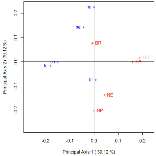
Figure 5. Correspondence plot that visually examines the departure from symmetry for Table 1; $C=150$.

The following points can be made from the configuration in Figure 5 on departures from symmetry in Table 3. Keeping in mind that this correspondence plot captures slightly more than three-quarters of the departures from symmetry in Table 3

• the purchase of the five coffee brands is different across the first and second purchases and so reflects the departure from symmetry that Bowker’s statistic shows,
• the greatest departure from symmetry is for the coffee brand “High Point” since “HP” and “hp” lie furthest from the origin than any of the four remaining brands. Thus, it is this brand that has undergone the greatest difference in purchasing preference over the two time periods,
• the coffee brands are ordered as follows based on the greatest to least departure from perfect symmetry: “High Point”, “Taster’s Choice”, ”Sanka”, “Nescafé” and “Brim”,
• therefore, “Brim” is the coffee brand that has the most similar purchasing pattern across the two time periods when the brands were purchased.  

Furthermore, Figure 5 shows that

• the purchasing preferences of the brands “Sanka” and “Taster’s Choice” are very similar on their first purchase as well as on their second purchase. This can be seen because of the close proximity of “sa” and “tc” on the left of the plot, and “SA” and “TC” on the right of the plot,
• the purchasing preferences of the brands “High Point” and “Nescafé” are similar (although not as similar as “SA” and “TC”) within each of the two purchases.

8. Discussion

When studying departures from symmetry between the categorical variables of a two-way contingency table there are many different techniques that can be considered. A common thread amongst many of them (especially over the past few decades) has been to partition the contingency table into a symmetric part ($\mathbf{Y}$) and an asymmetric, or skew-symmetric, part ($\mathbf{K}$) as (1) shows. While such a partition has appeared in the correspondence analysis literature, to the best of our knowledge the above technique is the first to formally link a meaningful measure of asymmetry when visualising departures from symmetry. Specifically, this paper has shown how Bowker’s statistic [14] plays a pivotal role in quantifying such departures in the context of correspondence analysis. Importantly, we also showed that by using Bowker’s statistic, we are able to capture departures from perfect symmetry relative to the amount of symmetry that lies between the variables.

In preparing this paper, we considered metrics that differ to those we described above. Like Greenacre [13], we adopted a metric involving the mean row-column marginal proportion. However, since Bowker’s statistic is independent of the row and column marginal information, consideration was given to $\widehat{\mathbf{P}}=\left(\mathbf{P}+{\mathbf{P}}^T\right)/2$. While using such a metric does not lead to the exact total inertia, it does provide an excellent approximation to it in some cases. It also provides additional features not available with the metric adopted above and so this is an interesting avenue to pursue in the future.

There are further extensions of the technique described above that can be considered at a later time. One such extension, and one that we raised at the end of Section 3, is to investigate the role of the Cressie–Read family of divergence statistics [21] for visualising departures from perfect symmetry using correspondence analysis. Doing so then will mean that one can consider “symmetry” (as opposed to “independence”) versions of the special cases of this family of divergence statistics, such as $G_S^2$, the Freeman–Tukey statistic [27] and other association measures, as alternatives to Bowker’s $X^2$ statistic. One can then consider measures of accuracy such as those described by Hubert and Arabie [28] for assessing how different members of this family compare.

Another possible avenue for future research is to extend the above technique in the case where one categorical variable is defined as a predictor variable and the other is its response variable. Such an approach provides a visual means of identifying departures from perfect symmetry using non-symmetrical correspondence analysis. While the approach described above is confined to examining departures from perfect symmetry between two cross-classified categorical variables, another natural extension is to consider adapting the above technique to analyse multi-way contingency tables. There is scope to investigate how this can be achieved in the context of multiple and multi-way correspondence analysis [6]. However, this extension, and the others we described, will be left for consideration at a later date.

References

- Agresti, A. Categorical Data Analysis, 2nd ed.; Wiley: New York, NY, USA, 2002. [Google Scholar]
- Anderson, E.B. The Statistical Analysis of Categorical Data; Springer: Berlin/Heidelberg, Germany, 1991. [Google Scholar]
- Bove, G. Asymmetrical multidimensional scaling and correspondence analysis for square tables. Stat. Appl. 1992, 4, 587–598. [Google Scholar]
- De Falguerolles, A.; van der Heijden, P.G.M. Reduced rank quasi-symmetry and quasi-skew symmetry: A generalized bi-linear model approach. Ann. Fac. Sci. Toulouse 2002, 11, 507–524. [Google Scholar] [CrossRef]
- Iki, K.; Yamamoto, K.; Tomizawa, S. Quasi-diagonal exponent symmetry model for square contingency tables with ordered categories. Stat. Probab. Lett. 2014, 92, 33–38. [Google Scholar] [CrossRef]
- Tomizawa, S. Two kinds of measures of departure from symmetry in square contingency tables having nominal categories. Stat. Sin. 1994, 4, 325–334. [Google Scholar]
- Yamamoto, H. A measure of departure from symmetry for multi-way contingency tables with nominal categories. Jpn. J. Biom. 2004, 25, 69–88. [Google Scholar] [CrossRef][Green Version]
- Yamamoto, K.; Shimada, F.; Tomizawa, S. Measure of departure from symmetry for the analysis of collapsed square contingency tables with ordered categories. J. Appl. Stat. 2015, 42, 866–875. [Google Scholar] [CrossRef]
- Arellano-Valle, R.B.; Contreras-Reyes, J.E.; Stehlik, M. Generalized skew-normal negentropy and its application to fish condition factor time series. Entropy 2017, 19, 528. [Google Scholar] [CrossRef]
- Nishisato, S. Optimal Quantification and Symmetry; Springer: Singapore, 2022. [Google Scholar]
- Constantine, A.G.; Gower, J.C. Graphical representation of asymmetry. Appl. Stat. 1978, 27, 297–304. [Google Scholar] [CrossRef]
- Gower, J.C. The analysis of asymmetry and orthogonality. In Recent Developments in Statistics; Barra, J.R., Brodeau, F., Romer, G., van Cutsem, B., Eds.; North-Holland: Amsterdam, The Netherlands, 1977; pp. 109–123. [Google Scholar]
- Greenacre, M. Correspondence analysis of square asymmetric matrices. J. R. Stat. Soc. Ser. C Appl. Stat. 2000, 49, 297–310. [Google Scholar] [CrossRef]
- Bowker, A.H. A test for symmetry in contingency tables. J. Am. Stat. Assoc. 1948, 43, 572–598. [Google Scholar] [CrossRef] [PubMed]
- Grover, R.; Srinivasan, V. A simultaneous approach to market segmentation and market structuring. J. Mark. Res. 1987, 24, 129–153. [Google Scholar] [CrossRef]
- Beh, E.J.; Lombardo, R. Correspondence Analysis: Theory, Practice and New Strategies; Wiley: Chichester, UK, 2014. [Google Scholar]
- McNemar, Q. Note on the sampling error of the difference between correlated proportions or percentages. Psychometrika 1947, 12, 153–157. [Google Scholar] [CrossRef] [PubMed]
- Bishop, Y.M.; Fienberg, S.E.; Holland, P.W. Discrete Multivariate Analysis: Theory and Practice; MIT Press: Cambridge, MA, USA, 1975. [Google Scholar]
- Lancaster, H.O. The Chi-squared Distribution; Wiley: Sydney, Australia, 1969. [Google Scholar]
- Plackett, R.L. The Analysis of Categorical Data; Charles Griffin and Company, Limited: London, UK, 1974. [Google Scholar]
- Cressie, N.A.C.; Read, T.R.C. Multinomial goodness-of-fit tests. J. R. Stat. Soc. Ser. B 1984, 46, 440–464. [Google Scholar] [CrossRef]
- Beh, E.J.; Lombardo, R. Correspondence Analysis and the Cressie–Read Family of Divergence Statistics. National Institute for Applied Statistics Reasearch Australia (NIASRA) Working Paper Series. 2022. Available online: https://www.uow.edu.au/niasra/publications/ (accessed on 19 May 2022).
- Ward, R.C.; Gray, L.J. Eigensystem computation for skew-symmetric matrices and a class of symmetric matrices. Acm Trans. Math. Softw. 1978, 4, 278–285. [Google Scholar] [CrossRef]
- Murnaghan, F.D.; Wintner, A. A canonical form for real matrices under orthogonal transformations. Proc. Natl. Acad. Sci. USA 1931, 17, 417–420. [Google Scholar] [CrossRef] [PubMed]
- Paardekooper, M.H.C. An eigenvalue algorithm for skew-symmetric matrices. Numer. Math. 1971, 17, 189–202. [Google Scholar] [CrossRef]
- Agresti, A. An Introduction to Categorical Data Analysis, 3rd ed.; Wiley: New York, NY, USA, 2019. [Google Scholar]
- Freeman, M.F.; Tukey, J.W. Transformations related to the angular and square root. Ann. Math. Stat. 1950, 21, 607–611. [Google Scholar] [CrossRef]
- Hubert, L.; Arabie, P. Comparing partitions. J. Classif. 1985, 2, 193–218. [Google Scholar] [CrossRef]
Publisher’s Note: MDPI stays neutral with regard to jurisdictional claims in published maps and institutional affiliations. |
© 2022 by the authors. Licensee MDPI, Basel, Switzerland. This article is an open access article distributed under the terms and conditions of the Creative Commons Attribution (CC BY) license (https://creativecommons.org/licenses/by/4.0/).