
TACDFSL: Task Adaptive Cross Domain Few-Shot Learning

Abstract
:1. Introduction
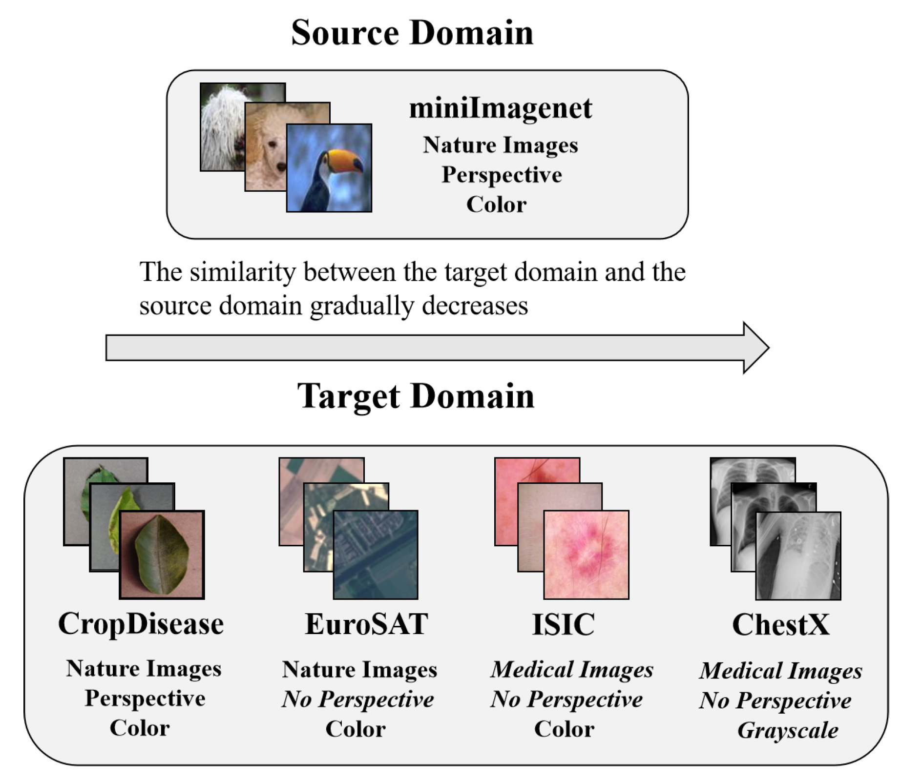
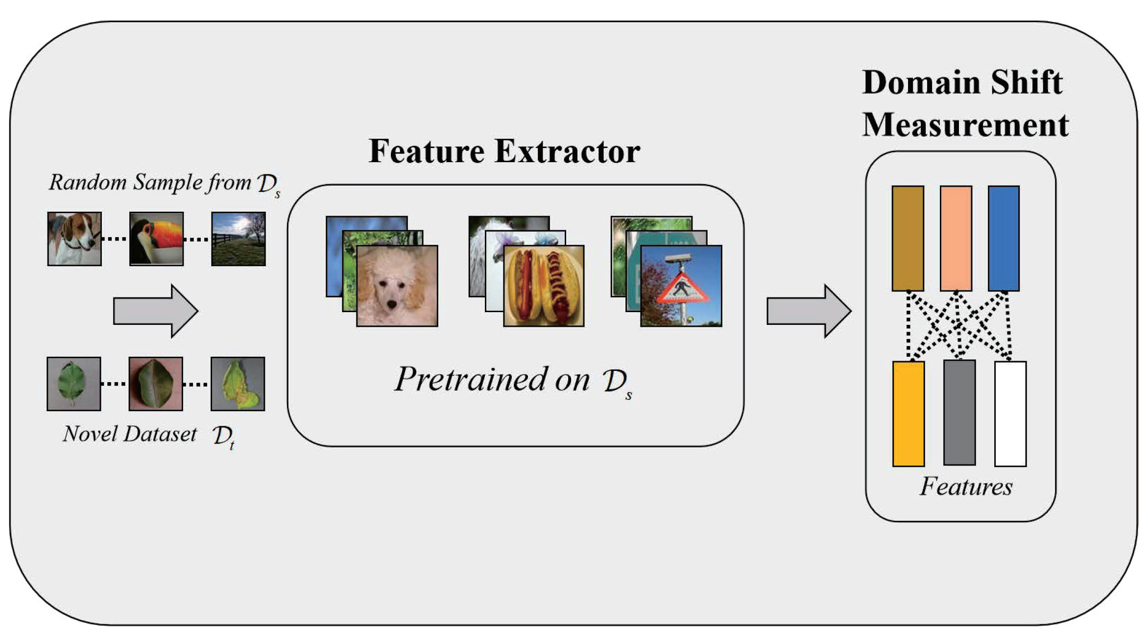
- For CDFSL, the domain shift between the source domain and the target domain is a key problem and domain shift is essentially a marginal distribution difference. However, the marginal distribution of the domain is implicit and unknown, so from the perspective of sample features, an empirical marginal distribution which is suitable for CDFSL is proposed, that is, WDMDS (Wasserstein Distance for Measuring Domain Shift) and MMDMDS (Maximum Mean Discrepancy for Measuring Domain Shift).
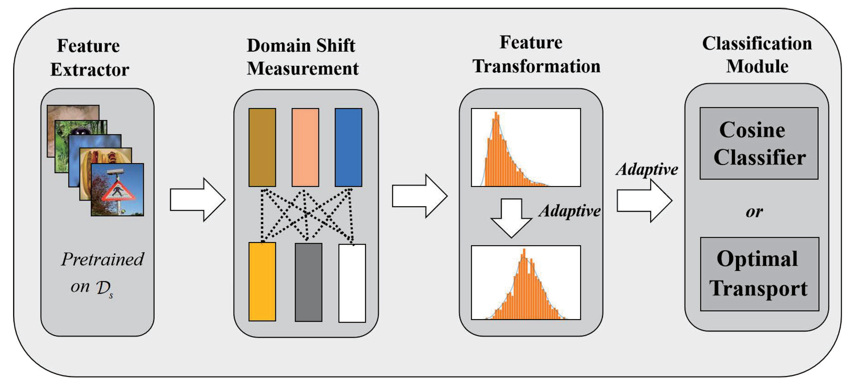
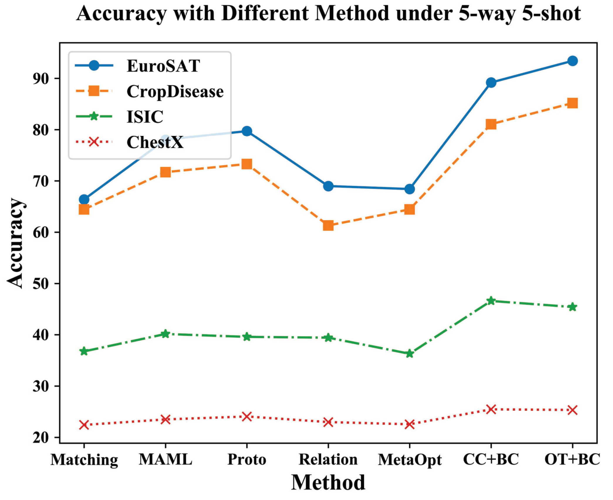
- Because of the large domain shift, the meta-learning-based method is not suitable for CDFSL. The rotation method to pre-train the feature extractor and fine-tune the novel task on the classifier is adopted, so that the model can fast and effectively generalize to novel tasks. The effectiveness of different classifiers on different datasets for CDFSL is compared. The research finds that selecting a classifier based on the basis of the empirical marginal distribution between domains is necessary. Hence, the Task Adaptive Cross Domain Few-Shot Learning (TACDFSL) is proposed.
- An adaptive feature distribution transformation is used to correct the left-biased feature distribution obtained by the convolutional neural network, which effectively improves image classification accuracy.
2. Related Work
3. Methodology
3.1. Feature Extractor
3.2. Empirical Marginal Distribution for CDFSL
3.2.1. Wasserstein Distance for Measuring Domain Shift (WDMDS)
3.2.2. Maximum Mean Discrepancy for Measuring Domain Shift (MMDMDS)
3.3. Adaptive Feature Distribution Transformation
3.4. Classifier Selection for CDFSL
3.4.1. Cosine Classifier
3.4.2. Optimal Transport
4. Experiments
4.1. Performance Evaluation with TACDFSL
4.2. Discussion
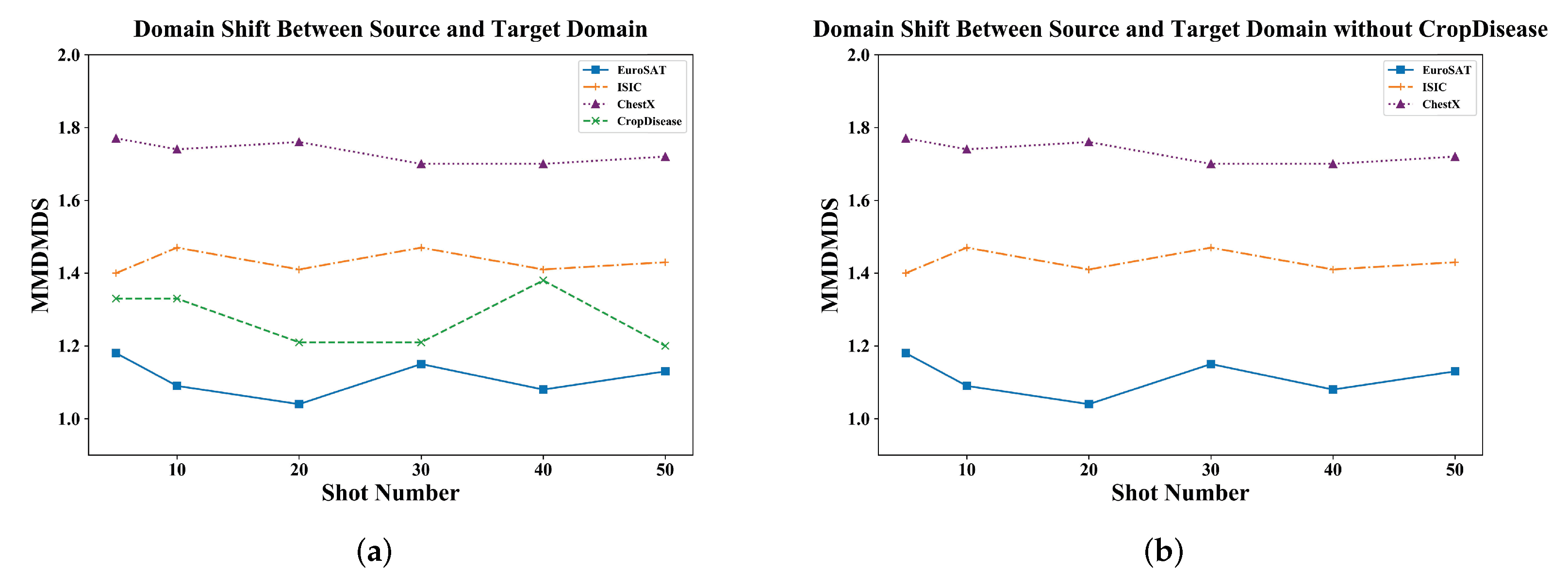
4.2.1. Measuring Domain Shift
4.2.2. Adaptive Feature Distribution Transformation Ablation Study
5. Conclusions
Author Contributions
Funding
Institutional Review Board Statement
Informed Consent Statement
Data Availability Statement
Conflicts of Interest
Abbreviations
| FSL | Few-Shot Learning |
| CDFSL | Cross Domain Few-Shot Learning |
| TACDFSL | Task Adaptive Cross Domain Few-Shot Learning |
| WDMDS | Wasserstein Distance for Measuring Domain Shift |
| MMDMDS | Maximum Mean Discrepancy for Measuring Domain Shift |
| CC | Cosine Classifier |
| OT | Optimal Transport |
References
- Fan, Z.; Yu, J.G.; Liang, Z. Fgn: Fully guided network for few-shot instance segmentation. In Proceedings of the 2020 IEEE/CVF Conference on Computer Vision and Pattern Recognition, Seattle, WA, USA, 13–19 June 2020; pp. 9172–9181. [Google Scholar]
- Ganea, D.A.; Boom, B.; Poppe, R. Incremental few-shot instance segmentation. In Proceedings of the 2021 IEEE/CVF Conference on Computer Vision and Pattern Recognition, Nashville, TN, USA, 20–25 June 2021; pp. 1185–1194. [Google Scholar]
- Simon, C.; Koniusz, P.; Nock, R. Adaptive subspaces for few-shot learning. In Proceedings of the 2020 IEEE/CVF Conference on Computer Vision and Pattern Recognition, Seattle, WA, USA, 13–19 June 2020; pp. 4136–4145. [Google Scholar]
- Jeong, T.; Kim, H. OOD-MAML: Meta-learning for few-shot out-of-distribution detection and classification. In Proceedings of the 2020 Conference on Neural Information Processing Systems, Online, 6–12 December 2020; Volume 33, pp. 3907–3916. [Google Scholar]
- Zhao, Y.; Wang, L.; Tian, Y. Few-shot neural architecture search. In Proceedings of the 2021 International Conference on Machine Learning, Online, 18–24 July 2021; pp. 12707–12718. [Google Scholar]
- Vinyals, O.; Blundell, C.; Lillicrap, T. Matching networks for one shot learning. In Proceedings of the Annual Conference on Neural Information Processing Systems, Barcelona, Spain, 5–10 December 2016; Volume 29. [Google Scholar]
- Snell, J.; Swersky, K.; Zemel, R. Prototypical networks for few-shot learning. In Proceedings of the Annual Conference on Neural Information Processing Systems, Long Beach, CA, USA, 4–9 December 2017; Volume 30. [Google Scholar]
- Sung, F.; Yang, Y.; Zhang, L. Learning to compare: Relation network for few-shot learning. In Proceedings of the 2018 IEEE/CVF Conference on Computer Vision and Pattern Recognition, Salt Lake City, UT, USA, 18–23 June 2018; pp. 1199–1208. [Google Scholar]
- Garcia, V.; Bruna, J. Few-shot learning with graph neural networks. In Proceedings of the 6th International Conference on Learning Representation, Vancouver, BC, Canada, 30 April–3 May 2018. [Google Scholar]
- Finn, C.; Abbeel, P.; Levine, S. Model-agnostic meta-learning for fast adaptation of deep networks. In Proceedings of the 2017 International Conference on Machine Learning, Sydney, Australia, 6–11 August 2017; pp. 1126–1135. [Google Scholar]
- Zhong, X.; Gu, C.; Huang, W. Complementing representation deficiency in few-shot image classification: A meta-learning approach. In Proceedings of the 25th International Conference on Pattern Recognition, Milan, Italy, 10–15 January 2021; pp. 2677–2684. [Google Scholar]
- Rajasegaran, J.; Khan, S.; Hayat, M. An incremental task-agnostic meta-learning approach. In Proceedings of the 2020 Conference on Computer Vision and Pattern Recognition, Seattle, WA, USA, 13–19 June 2020; pp. 13588–13597. [Google Scholar]
- Sugandh, U.; Khari, M.; Nigam, S. The integration of blockchain and IoT edge devices for smart agriculture: The challenges and use cases. Adv. Comput. 2022. [Google Scholar] [CrossRef]
- Sugandh, U.; Khari, M.; Nigam, S. How Blockchain Technology Can Transfigure the Indian Agriculture Sector: A Review. In Handbook of Green Computing and Blockchain Technologies; CRC Press: Boca Raton, FL, USA, 2022; pp. 69–88. [Google Scholar]
- Srivastava, S.; Khari, M.; Crespo, R.G.; Chaudhary, G.; Arora, P. Concepts and Real-Time Applications of Deep Learning; Springer International Publishing: Cham, Switzerland, 2021. [Google Scholar]
- Tseng, H.Y.; Lee, H.Y. Cross-Domain Few-Shot Classification via Learned Feature-Wise Transformation. In Proceedings of the 8th International Conference on Learning Representations, Addis Ababa, Ethiopia, 26–30 April 2020. [Google Scholar]
- Wah, C.; Branson, S.; Welinder, P. The Caltech-UCSD Birds-200-2011 Dataset; California Institute of Technology: Pasadena, CA, USA, 2011. [Google Scholar]
- Chen, W.Y.; Liu, Y.C.; Kira, Z. A closer look at few-shot classification. In Proceedings of the 7th International Conference on Learning Representations, New Orleans, LA, USA, 6–9 May 2019. [Google Scholar]
- Guo, Y.; Codella, N.C.; Karlinsky, L. A broader study of cross-domain few-shot learning. In Proceedings of the 2020 European Conference on Computer Vision, Glasgow, UK, 23–28 August 2020; pp. 124–141. [Google Scholar]
- Deng, J.; Dong, W.; Socher, R. A large-scale hierarchical image database. In Proceedings of the 2009 Conference on Computer Vision and Pattern Recognition, Miami, FL, USA, 20–25 June 2009; pp. 248–255. [Google Scholar]
- Mohanty, S.P.; Hughes, D.P.; Salathé, M. Using deep learning for image-based plant disease detection. Front. Plant Sci. 2016, 7, 1419. [Google Scholar] [CrossRef] [PubMed] [Green Version]
- Helber, P.; Bischke, B.; Dengel, A. Eurosat: A novel dataset and deep learning benchmark for land use and land cover classification. IEEE J. Sel. Top. Appl. Earth Obs. Remote Sens. 2019, 12, 2217–2226. [Google Scholar] [CrossRef] [Green Version]
- Tschandl, P.; Rrsendahl, C.; Kittler, H. The ham10000 dataset, a large collection of multi-source dermatoscopic images of common pigmented skin lesions. Sci. Data 2018, 5, 1–9. [Google Scholar] [CrossRef] [PubMed]
- Wang, X.; Peng, Y.; LU, L. Chestx-ray8: Hospital-scale chest x-ray database and benchmarks on weakly-supervised classification and localization of common thorax diseases. In Proceedings of the 2017 Conference on Computer Vision and Pattern Recognition, Honolulu, HI, USA, 21–26 July 2017; pp. 2097–2106. [Google Scholar]
- Rusu, A.A.; Rao, D.; Sygnowski, J. Meta-learning with latent embedding optimization. In Proceedings of the 7th International Conference on Learning Representations, New Orleans, LA, USA, 6–9 May 2019. [Google Scholar]
- Vuorio, R.; Sun, S.H.; Hu, H. Multimodal model-agnostic meta-learning via task-aware modulation. In Proceedings of the 2019 Conference on Neural Information Processing Systems, Vancouver, BC, Canada, 8–14 December 2019; Volume 32. [Google Scholar]
- Tseng, H.Y.; De, M.S.; Tremblay, J. Few-shot viewpoint estimation. In Proceedings of the 31st British Machine Vision Virtual Conference, Online, 7–10 September 2020. [Google Scholar]
- Wang, Y.X.; Girshick, R.; Hebert, M. Low-shot learning from imaginary data. In Proceedings of the 2018 Conference on Computer Vision and Pattern Recognition, Salt Lake City, UT, USA, 18–22 June 2018; pp. 7278–7286. [Google Scholar]
- Alfassy, A.; Karlinsky, L.; Aides, A. Laso: Label-set operations networks for multi-label few-shot learning. In Proceedings of the 2019 Conference on Computer Vision and Pattern Recognition, Long Beach, CA, USA, 16–20 June 2019; pp. 6548–6557. [Google Scholar]
- Mangla, P.; Kumari, N.; Sinha, A. Charting the right manifold: Manifold mixup for few-shot learning. In Proceedings of the 2022 Winter Conference on Applications of Computer Vision, Waikoloa, HI, USA, 4–8 January 2022; pp. 2218–2227. [Google Scholar]
- Hu, Y.; Gripon, V.; Pateux, S. Leveraging the feature distribution in transfer-based few-shot learning. In Proceedings of the 2021 International Conference on Learning Representations, Vienna, Austria, 3–7 May 2021; pp. 487–499. [Google Scholar]
- Yang, S.; Liu, L.; Xu, M. Free lunch for few-shot learning: Distribution calibration. In Proceedings of the 2021 International Conference on Learning Representations, Vienna, Austria, 3–7 May 2021. [Google Scholar]
- Phoo, C.P.; Hariharan, B. Self-training for few-shot transfer across extreme task differences. In Proceedings of the 2021 International Conference on Learning Representations, Vienna, Austria, 3–7 May 2021. [Google Scholar]
- Wang, A.; Liu, C.; Xue, D. Hyperspectral Image Classification Based on Cross-Scene Adaptive Learning. Symmetry 2021, 13, 1817. [Google Scholar] [CrossRef]
- Hsu, H.K.; Yao, C.H.; Tsai, Y.H. Progressive domain adaptation for object detection. In Proceedings of the 2020 Winter Conference on Applications of Computer Vision, Snowmass Village, CO, USA, 2–5 March 2020; pp. 749–757. [Google Scholar]
- Wang, F.; Chai, G.; Li, Q. An Efficient Deep Unsupervised Domain Adaptation for Unknown Malware Detection. Symmetry 2022, 14, 296. [Google Scholar] [CrossRef]
- Fickinger, A.; Cohen, S.; Russell, S. Cross-Domain Imitation Learning via Optimal Transport. In Proceedings of the 2022 International Conference on Learning Representations, Online, 25–29 April 2022. [Google Scholar]
- Rubner, Y.; Tomasi, C.; Guibas, L.J. The earth mover’s distance as a metric for image retrieval. Int. J. Comput. Vis. 2000, 40, 99–121. [Google Scholar] [CrossRef]
- Borgwardt, K.M.; Gretton, A.; Rasch, M.J. Integrating structured biological data by kernel maximum mean discrepancy. Bioinformatics 2006, 22, e49–e57. [Google Scholar] [CrossRef] [PubMed] [Green Version]
- Gretton, A.; Sejdinovic, D.; Strathmann, H. Optimal kernel choice for large-scale two-sample tests. In Proceedings of the 2012 Annual Conference on Neural Information Processing Systems, Lake Tahoe, NV, USA, 3–8 December 2021; Volume 25. [Google Scholar]
- Duan, L.; Tsang, I.W.; Xu, D. Domain transfer multiple kernel learning. IEEE Trans. Pattern Anal. Mach. Intell. 2012, 34, 465–479. [Google Scholar] [CrossRef] [PubMed]
- Box, G.E.P.; Cox, D.R. An analysis of transformations. J. R. Stat. Soc. Ser. B Stat. Methodol. 1964, 26, 211–243. [Google Scholar] [CrossRef]


| CropDisease 5-Way | EuroSAT5-Way | |||||
| Methods | 5-Shot | 20-Shot | 50-Shot | 5-Shot | 20-Shot | 50-Shot |
| MatchingNet † | 66.39 ± 0.78 | 76.38 ± 0.67 | 58.53 ± 0.73 | 64.45 ± 0.63 | 77.10 ± 0.57 | 54.44 ± 0.67 |
| MatchingNet+FWT † | 62.74 ± 0.90 | 74.90 ± 0.71 | 75.68 ± 0.78 | 56.04 ± 0.65 | 63.38 ± 0.69 | 62.75 ± 0.76 |
| MAML † | 78.05 ± 0.68 | 89.75 ± 0.42 | - | 71.70 ± 0.72 | 81.95 ± 0.55 | - |
| ProtoNet † | 79.72 ± 0.67 | 88.15 ± 0.51 | 90.81 ± 0.43 | 73.29 ± 0.71 | 82.27 ± 0.57 | 80.48 ± 0.57 |
| ProtoNet+FWT † | 72.72 ± 0.70 | 85.82 ± 0.51 | 87.17 ± 0.50 | 67.34 ± 0.76 | 75.74 ± 0.70 | 78.64 ± 0.57 |
| RelationNet † | 68.99 ± 0.75 | 80.45 ± 0.64 | 85.08 ± 0.53 | 61.31 ± 0.72 | 74.43 ± 0.66 | 74.91 ± 0.58 |
| RelationNet+FWT † | 64.91 ± 0.79 | 78.43 ± 0.59 | 81.14 ± 0.56 | 61.16 ± 0.70 | 69.40 ± 0.64 | 73.84 ± 0.60 |
| MetaOpt † | 68.41 ± 0.73 | 82.89 ± 0.54 | 91.76 ± 0.38 | 64.44 ± 0.73 | 79.19 ± 0.62 | 83.62 ± 0.58 |
| Backbone | 80.61 ± 0.70 | 89.61 ± 0.48 | 91.97 ± 0.43 | 76.74 ± 0.66 | 83.74 ± 0.52 | 86.49 ± 0.47 |
| CC + Box-Cox | 89.20 ± 0.54 | 95.24 ± 0.33 | 96.78 ± 0.26 | 81.08 ± 0.61 | 88.72 ± 0.40 | 91.40 ± 0.36 |
| OT + Box-Cox | 93.42 ± 0.55 | 95.49 ± 0.39 | 95.88 ± 0.35 | 85.19 ± 0.67 | 87.87 ± 0.49 | 89.07 ± 0.43 |
| ISIC 5-Way | ChestX 5-Way | |||||
| Methods | 5-Shot | 20-Shot | 50-Shot | 5-Shot | 20-Shot | 50-Shot |
| MatchingNet † | 36.74 ± 0.53 | 45.72 ± 0.53 | 54.58 ± 0.65 | 22.40 ± 0.70 | 23.61 ± 0.86 | 22.12 ± 0.88 |
| MatchingNet+FWT † | 30.40 ± 0.48 | 32.01 ± 0.48 | 33.17 ± 0.43 | 21.26 ± 0.31 | 23.23 ± 0.37 | 23.01 ± 0.34 |
| MAML † | 40.13 ± 0.58 | 52.36 ± 0.57 | - | 23.48 ± 0.96 | 27.53 ± 0.43 | - |
| ProtoNet † | 39.57 ± 0.57 | 49.50 ± 0.55 | 51.99 ± 0.52 | 24.05 ± 1.01 | 28.21 ± 1.15 | 29.32 ± 1.12 |
| ProtoNet+FWT † | 38.87 ± 0.52 | 43.78 ± 0.47 | 49.84 ± 0.51 | 23.77 ± 0.42 | 26.87 ± 0.43 | 30.12 ± 0.46 |
| RelationNet † | 39.41 ± 0.58 | 41.77 ± 0.49 | 49.32 ± 0.51 | 22.96 ± 0.88 | 26.63 ± 0.92 | 28.45 ± 1.20 |
| RelationNet+FWT † | 35.54 ± 0.55 | 43.31 ± 0.51 | 46.38 ± 0.53 | 22.74 ± 0.40 | 26.75 ± 0.41 | 27.56 ± 0.40 |
| MetaOpt † | 36.28 ± 0.50 | 49.42 ± 0.60 | 54.80 ± 0.54 | 22.53 ± 0.91 | 25.53 ± 1.02 | 29.35 ± 0.99 |
| Backbone | 37.42 ± 0.54 | 44.67 ± 0.53 | 49.79 ± 0.55 | 23.88 ± 0.41 | 27.04 ± 0.45 | 30.78 ± 0.50 |
| CC + Box-Cox | 46.57 ± 0.61 | 56.18 ± 0.59 | 61.59 ± 0.56 | 25.44 ± 0.46 | 30.08 ± 0.52 | 32.92 ± 0.52 |
| OT + Box-Cox | 45.39 ± 0.67 | 53.15 ± 0.59 | 56.68 ± 0.58 | 25.32 ± 0.48 | 29.17 ± 0.52 | 31.75 ± 0.51 |
| CropDisease 5-Way | EuroSAT 5-Way | |||||||
| Methods | 1-Shot | 5-Shot | 20-Shot | 50-Shot | 1-Shot | 5-Shot | 20-Shot | 50-Shot |
| WDMDS | 1.10 ± 0.01 | 1.00 ± 0.00 | - | - | 0.89 ± 0.01 | 0.87 ± 0.01 | - | - |
| MMDMDS | - | 1.33 ± 0.01 | 1.21 ± 0.01 | 1.20 ± 0.01 | - | 1.18 ± 0.01 | 1.04 ± 0.01 | 1.13 ± 0.01 |
| ISIC 5-Way | ChestX 5-Way | |||||||
| Methods | 1-Shot | 5-Shot | 20-Shot | 50-Shot | 1-Shot | 5-Shot | 20-Shot | 50-Shot |
| WDMDS | 0.97 ± 0.01 | 0.95 ± 0.00 | - | - | 1.14 ± 0.01 | 1.07 ± 0.00 | - | - |
| MMDMDS | - | 1.40 ± 0.01 | 1.41 ± 0.01 | 1.43 ± 0.01 | - | 1.77 ± 0.00 | 1.76 ± 0.00 | 1.72 ± 0.00 |
| Dataset | 5-Shot | 10-Shot | 20-Shot | 30-Shot | 40-Shot | 50-Shot |
|---|---|---|---|---|---|---|
| CropDisease | 1.33 ± 0.01 | 1.33 ± 0.01 | 1.21 ± 0.01 | 1.21 ± 0.01 | 1.38 ± 0.01 | 1.20 ± 0.01 |
| EuroSAT | 1.18 ± 0.01 | 1.09 ± 0.01 | 1.04 ± 0.01 | 1.15 ± 0.01 | 1.08 ± 0.01 | 1.13 ± 0.01 |
| ISIC | 1.40 ± 0.01 | 1.47 ± 0.01 | 1.41 ± 0.01 | 1.47 ± 0.01 | 1.41 ± 0.01 | 1.43 ± 0.01 |
| ChestX | 1.77 ± 0.00 | 1.74 ± 0.00 | 1.76 ± 0.00 | 1.70 ± 0.00 | 1.70 ± 0.00 | 1.72 ± 0.00 |
| CropDisease 5-Way | EuroSAT 5-Way | |||||
| Methods | 5-Shot | 20-Shot | 50-Shot | 5-Shot | 20-Shot | 50-Shot |
| CC | 86.31 ± 0.63 | 93.67 ± 0.36 | 95.84 ± 0.26 | 80.49 ± 0.66 | 88.12 ± 0.46 | 90.76 ± 0.37 |
| CC + Box-Cox | 89.20 ± 0.54 | 95.24 ± 0.33 | 96.78 ± 0.26 | 81.62 ± 0.60 | 88.95 ± 0.40 | 91.40 ± 0.36 |
| OT | 88.06 ± 0.74 | 90.80 ± 0.55 | 92.50 ± 0.44 | 80.68 ± 0.78 | 84.53 ± 0.60 | 86.39 ± 0.54 |
| OT + Box-Cox | 93.42 ± 0.55 | 95.49 ± 0.39 | 95.88 ± 0.35 | 85.19 ± 0.67 | 87.87 ± 0.49 | 89.07 ± 0.43 |
| ISIC 5-Way | ChestX 5-Way | |||||
| Methods | 5-Shot | 20-Shot | 50-Shot | 5-Shot | 20-Shot | 50-Shot |
| CC | 42.11 ± 0.59 | 52.88 ± 0.59 | 57.86 ± 0.56 | 24.60 ± 0.40 | 29.61 ± 0.50 | 32.30 ± 0.55 |
| CC + Box-Cox | 46.57 ± 0.61 | 56.18 ± 0.59 | 61.59 ± 0.56 | 25.44 ± 0.46 | 30.08 ± 0.52 | 32.92 ± 0.52 |
| OT | 38.60 ± 0.65 | 44.36 ± 0.60 | 47.98 ± 0.59 | 23.56 ± 0.44 | 26.81 ± 0.46 | 28.96 ± 0.48 |
| OT + Box-Cox | 45.39 ± 0.67 | 53.15 ± 0.59 | 56.68 ± 0.58 | 25.32 ± 0.48 | 29.17 ± 0.52 | 31.75 ± 0.51 |
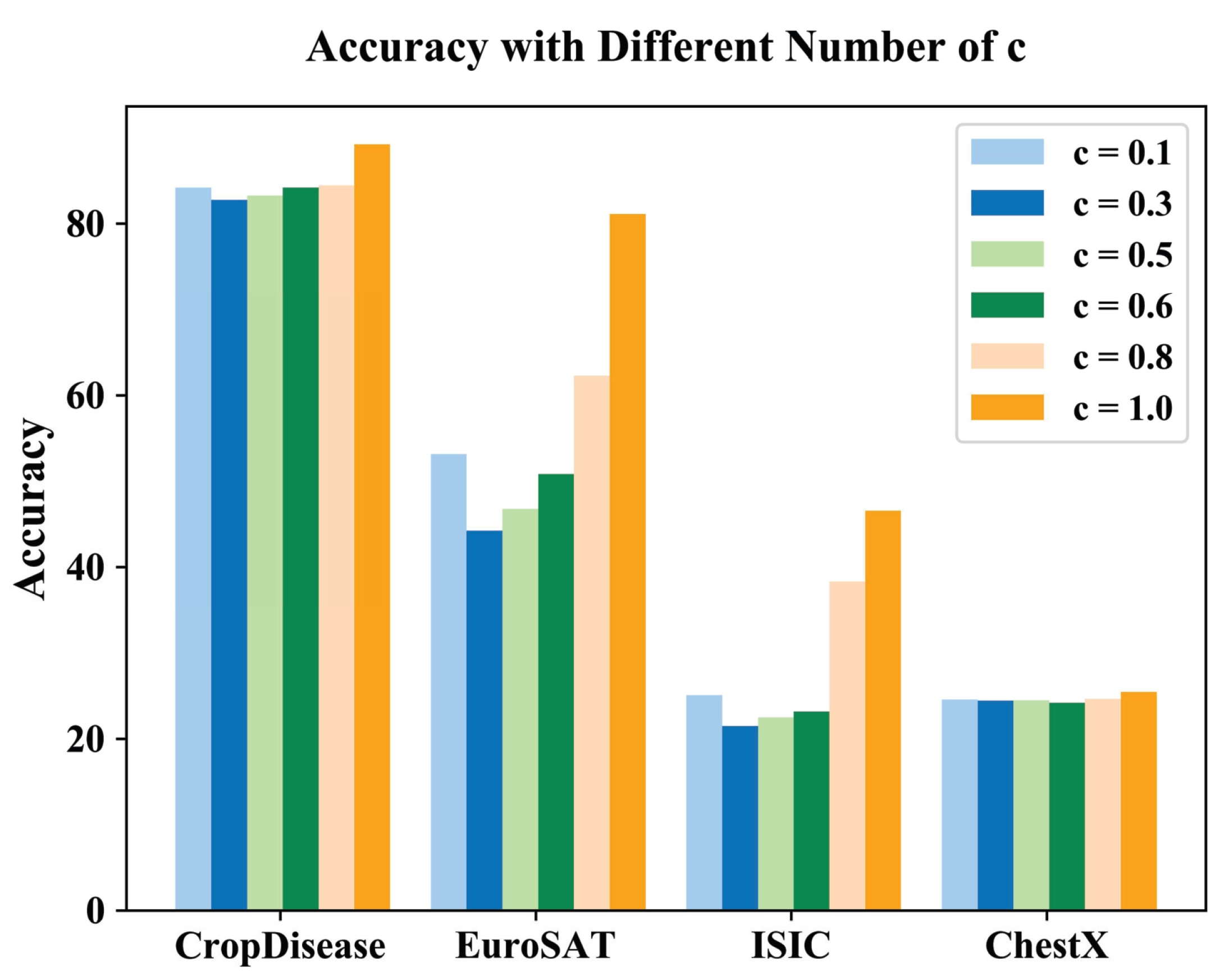
| 5-Shot | 10-Shot | 20-Shot | 30-Shot | 40-Shot | 50-Shot | |
|---|---|---|---|---|---|---|
| Dataset | ||||||
| CropDisease | 84.18 ± 0.68 | 82.75 ± 0.73 | 83.25 ± 0.73 | 84.20 ± 0.70 | 84.45 ± 0.74 | 89.20 ± 0.54 |
| EuroSAT | 53.14 ± 0.89 | 44.24 ± 0.88 | 46.78 ± 0.87 | 50.81 ± 0.88 | 62.26 ± 0.87 | 81.08 ± 0.61 |
| ISIC | 25.04 ± 0.42 | 21.46 ± 0.30 | 22.47 ± 0.32 | 23.14 ± 0.39 | 38.33 ± 0.57 | 46.57 ± 0.61 |
| ChestX | 24.54 ± 0.40 | 24.40 ± 0.41 | 24.45 ± 0.41 | 24.18 ± 0.40 | 24.62 ± 0.41 | 25.44 ± 0.46 |
Publisher’s Note: MDPI stays neutral with regard to jurisdictional claims in published maps and institutional affiliations. |
© 2022 by the authors. Licensee MDPI, Basel, Switzerland. This article is an open access article distributed under the terms and conditions of the Creative Commons Attribution (CC BY) license (https://creativecommons.org/licenses/by/4.0/).
Share and Cite
Zhang, Q.; Jiang, Y.; Wen, Z. TACDFSL: Task Adaptive Cross Domain Few-Shot Learning. Symmetry 2022, 14, 1097. https://doi.org/10.3390/sym14061097
Zhang Q, Jiang Y, Wen Z. TACDFSL: Task Adaptive Cross Domain Few-Shot Learning. Symmetry. 2022; 14(6):1097. https://doi.org/10.3390/sym14061097
Chicago/Turabian StyleZhang, Qi, Yingluo Jiang, and Zhijie Wen. 2022. "TACDFSL: Task Adaptive Cross Domain Few-Shot Learning" Symmetry 14, no. 6: 1097. https://doi.org/10.3390/sym14061097
APA StyleZhang, Q., Jiang, Y., & Wen, Z. (2022). TACDFSL: Task Adaptive Cross Domain Few-Shot Learning. Symmetry, 14(6), 1097. https://doi.org/10.3390/sym14061097