
Bayesian Inferential Approaches and Bootstrap for the Reliability and Hazard Rate Functions under Progressive First-Failure Censoring for Coronavirus Data from Asymmetric Model

 ,
,  ,
,  , ,
, ,
Abstract
1. Introduction
- WFr follows the Weibull inverse exponential model.
- WFr is the exponential Frechet model.
- WFr refers to the Weibull inverse Rayleigh model.
- WFr reduces to the exponential inverse Rayleigh model.
- WFr follows the exponential inverse exponential model.
2. Maximum Likelihood Inference
- Begin with a guess initial values and set .
- Calculate and the observed Fisher information matrix given in Section 2.1.
- Update as
- Set and then go back to Step 1.
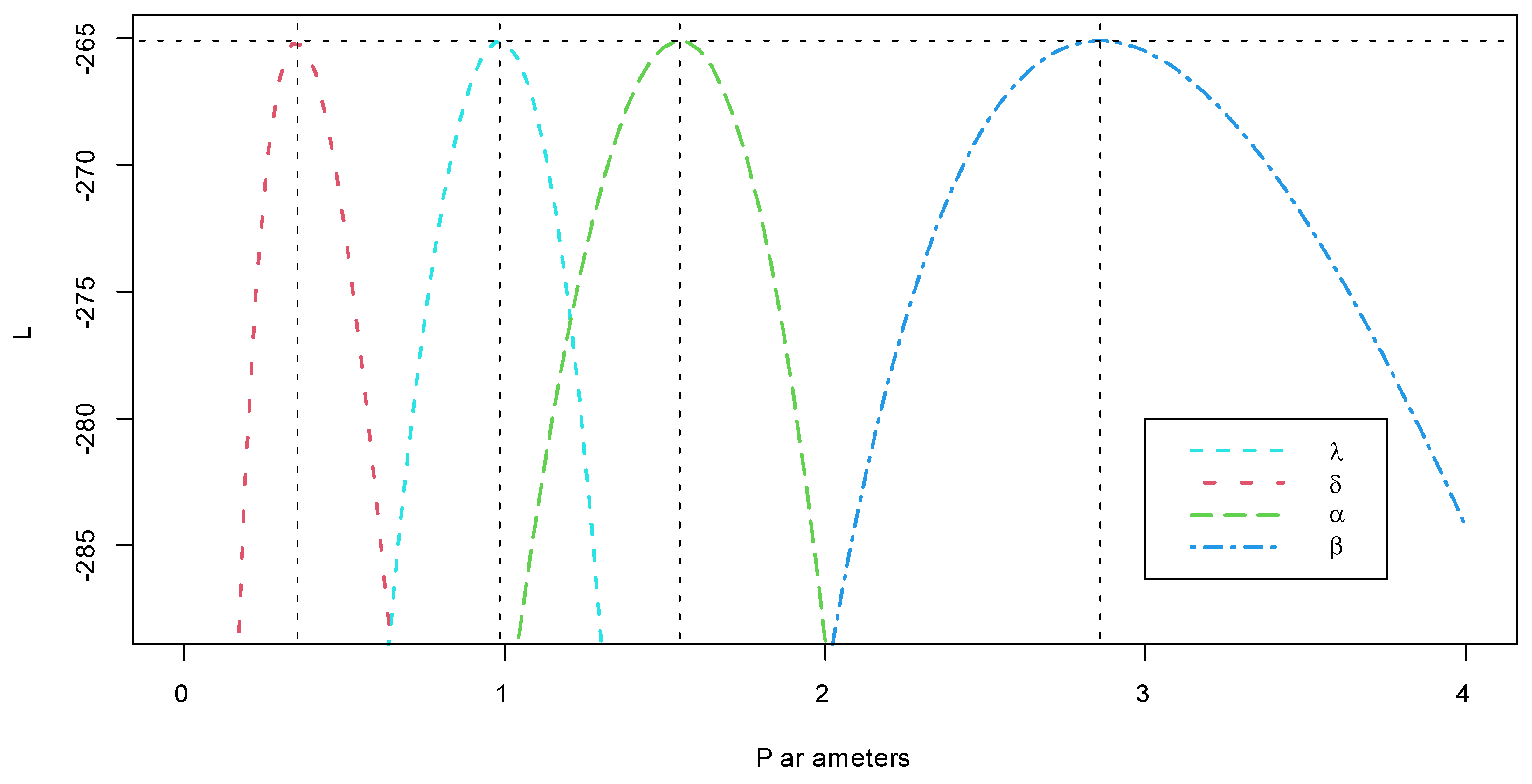
- Continue the iterative steps until is smaller than a threshold value. The final estimates of and are the MLE of the parameters, denoted as and .
2.1. Asymptotic Confidence Intervals
3. Parametric Bootstrap Methods
3.1. Percentile Bootstrap
- From the original data , compute the MLEs of the unknown parameters and by solving the nonlinear Equations (6)–(10), denoted the estimates as .
- Use and to generate PFFC sample with the same values of and compute the bootstrap estimates .
- Repeat Step 2 N times; then, we have
- Arrange all components in ascending order; the bootstrap estimates are .
- Let be the CDF of . Define for given x. Then, two-side percentile confidence intervals of given by
3.2. Bootstrap-t
- 1,2.
- The same as the percentile bootstrap.
- 3.
- Compute the t-statistics where obtained using the FIM for , , , and delta method for and .
- 4.
- Repeat Steps 2, 3, 4 N times; then, we have .
- 5.
- Let be the CDF of . Define for given x. Then, two-side bootstrap-t confidence intervals of , , , or given by
4. Bayes Inference
- Use the MLEs as the initial value, denoted by and .
- Set
- Generate from Gamma .
- Using M-H algorithm, generate and from and , respectively, with the normal distributions , and .
- (a)
- Generate from from and from .
- (b)
- Evaluate the acceptance probabilities
- (c)
- Generate a and from a Uniform distribution.
- (d)
- If , accept the proposal and set , else set .
- (e)
- If , accept the proposal and set , else set .
- (f)
- If , accept the proposal and set , else set .
- Compute and as
- Set .
- Reiterate Steps (3)–(6) M times. The first simulated varieties are ignored to remove the affection of the selection of initial value and to guarantee the convergence. Then, the selected sample is and for sufficiently large M, forms an approximate posterior sample which can be used to develop the Bayesian inference.
- Under SE and LINEX loss functions, the approximate Bayes estimate of (where and ) can be obtained bywhere is the burn-in period and and .
- To compute the CRIs of , order as . Then, the CRIs of can be given by
5. Simulation Study
- CS I:
- for
- CS II:
- for if m odd; for if m even.
- CS III:
- for
- The Bayes estimates have the smallest MSEs and ALs for the unknown quantities , , , and . Hence, Bayes estimates performed better than the MLEs and bootstrap methods.
- The Bootstrap methods performed better than the ML method of in terms of the MSEs and ALs. Moreover, boot-t performs better than boot-p in terms of the MSEs and ALs.
- The Bayes estimate under LINEX with provides better estimates for because of having the smallest MSEs.
- The Bayes estimates of under LINEX for the choice performed better than their estimates for the choice in the sense of having smaller MSEs.
- From all of the tables, we observe that as the group size k increases, the MSEs and ALs associated with increase.
- For fixed sample sizes and observed failures, the first scheme I is the best scheme in the sense of having smaller MSEs and ALs.
- The MLE, bootstrap and Bayesian methods have very close estimates and their ACIs have quite high CPs (around ). Moreover, the Bayesian CRIs have the highest CPs.
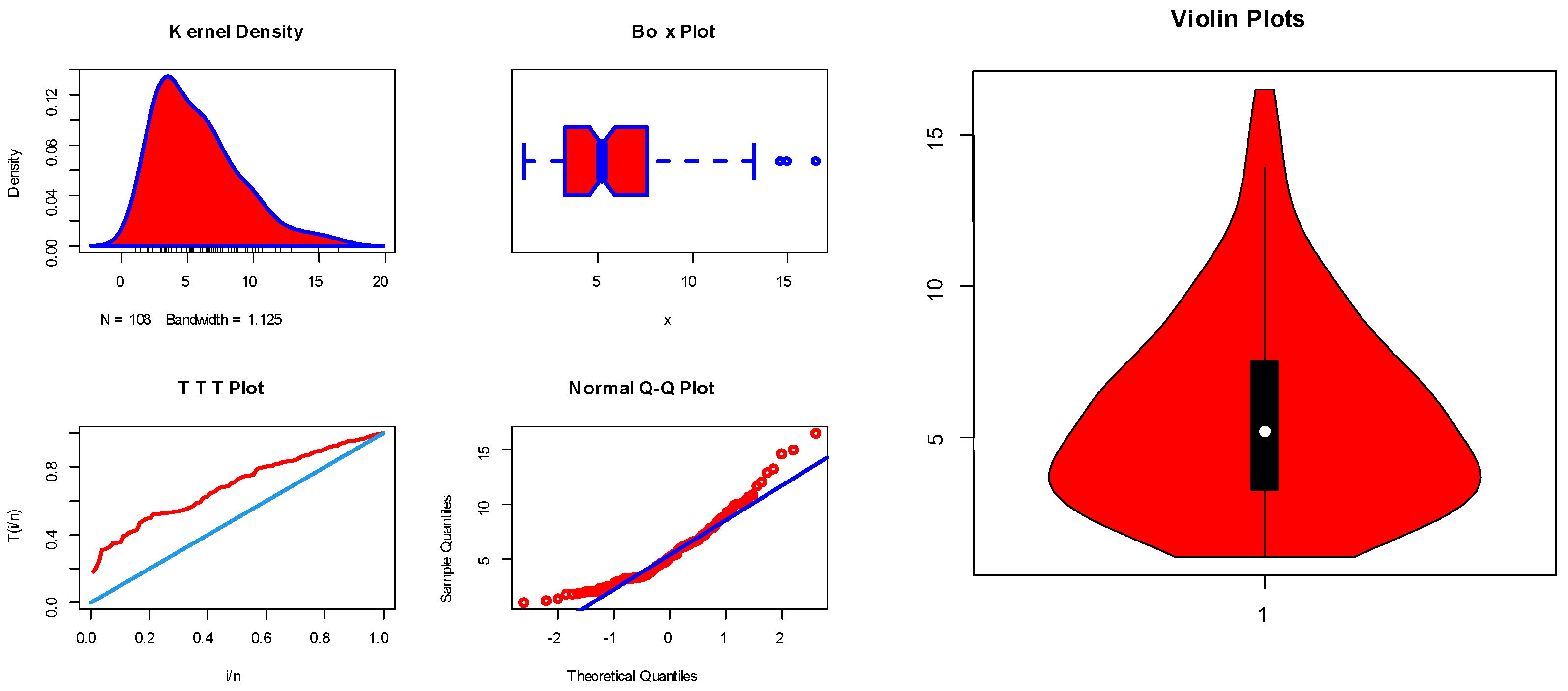
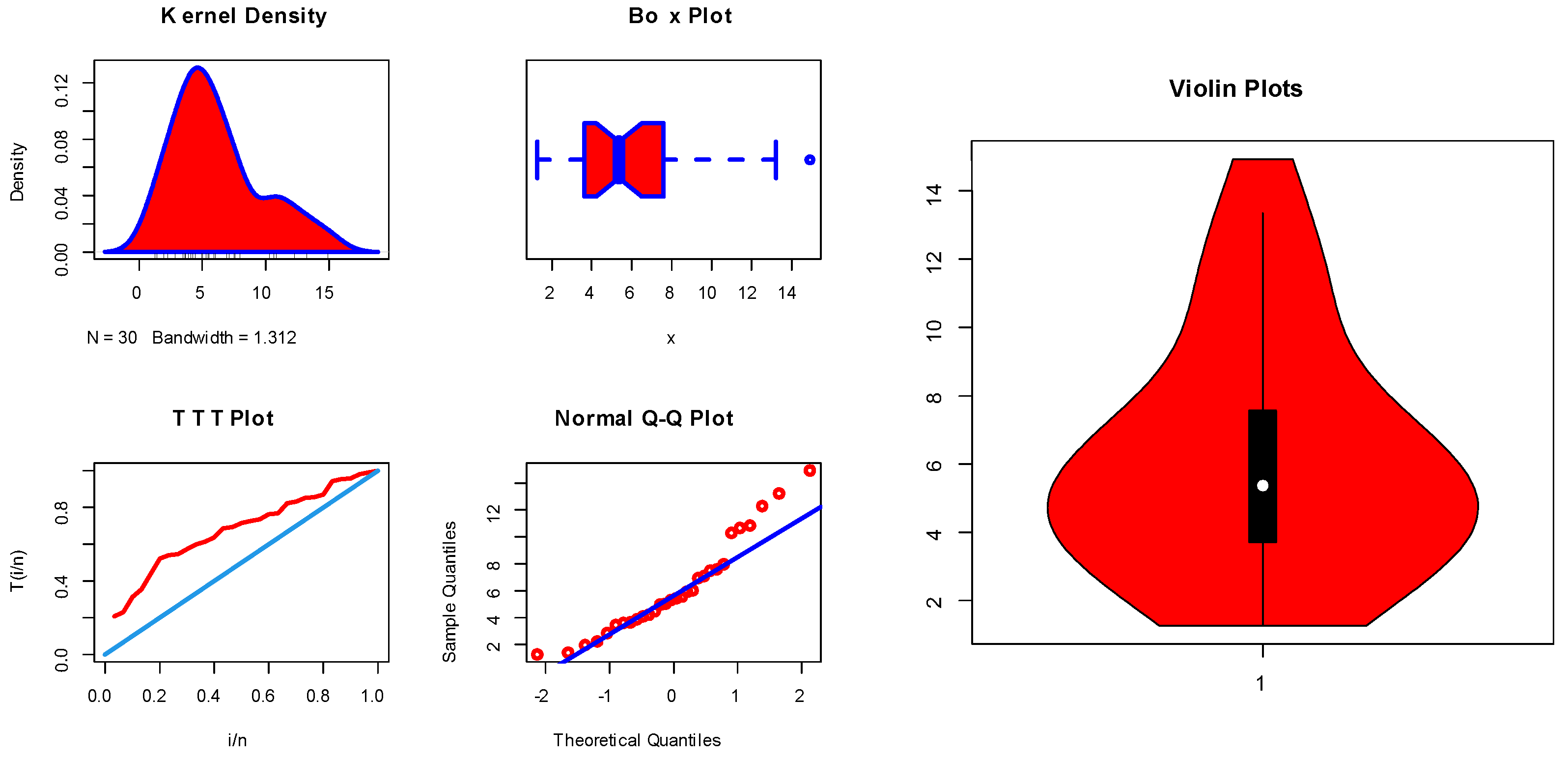
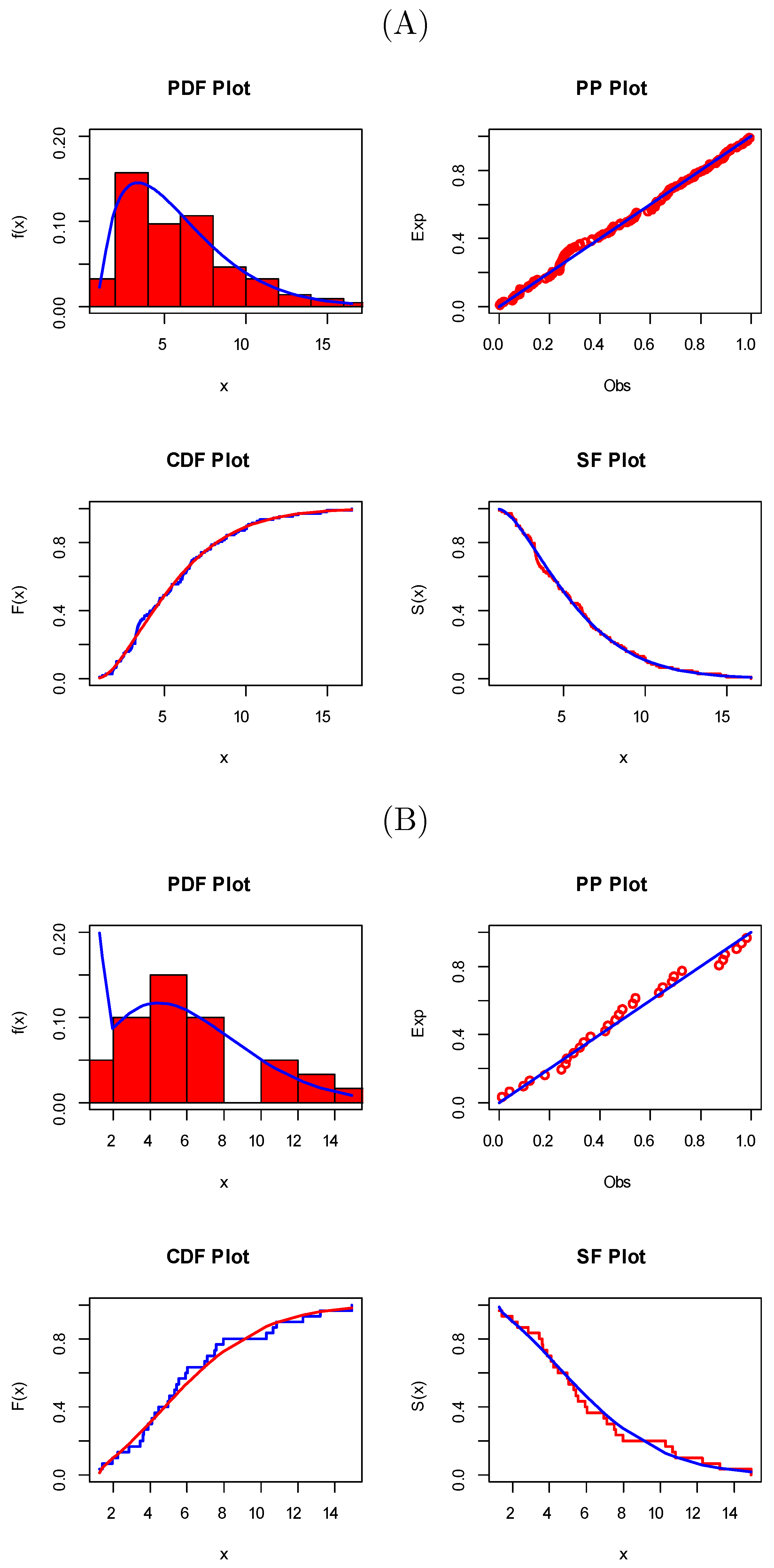
6. Applications of COVID-19 Data
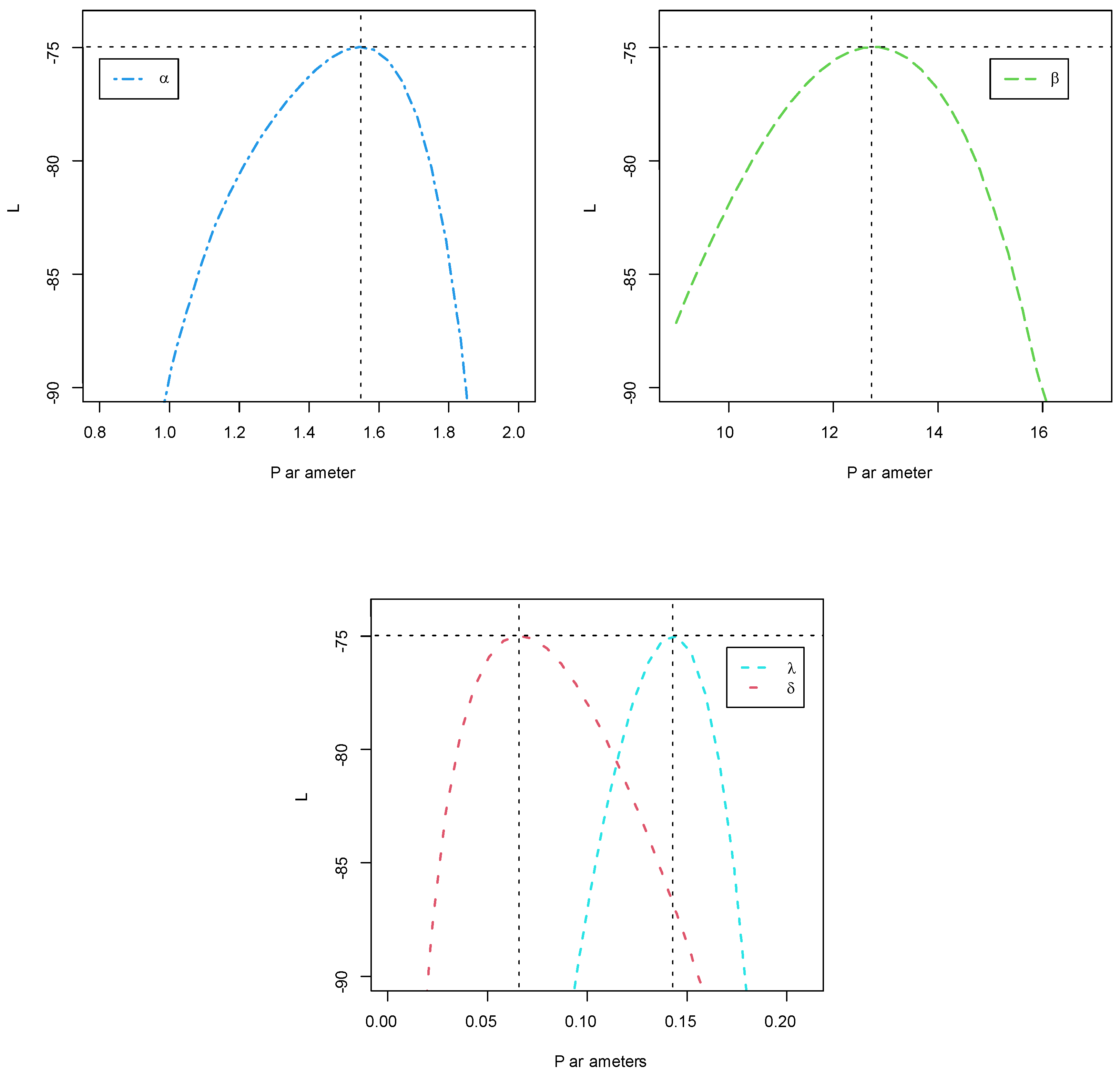
- The model under study fits the data very well, and this is quite clear from the figures.
- The estimation of the four methods is somewhat similar, with very slight differences, which gives a good impression to the reader.
- Approximate confidence intervals are good, and all point estimates fall within them. In addition, there are slight differences in the lengths of the intervals, as expected.
7. Conclusions
Author Contributions
Funding
Institutional Review Board Statement
Informed Consent Statement
Data Availability Statement
Acknowledgments
Conflicts of Interest
References
- Balakrishnan, N.; Sandhu, R.A. A simple simulation algorithm for generating progressively type-II censored samples. Am. Stat. 1995, 49, 229–230. [Google Scholar]
- Fu, J.; Xu, A.; Tang, Y. Objective Bayesian analysis of Pareto distribution under progressive Type-II censoring. Stat. Probab. Lett. 2012, 82, 1829–1836. [Google Scholar] [CrossRef]
- Chen, P.; Xu, A.; Ye, Z. Generalized fiducial inference for accelerated life tests with Weibull distribution and progressively type-II censoring. IEEE Trans. Reliab. 2016, 65, 1737–1744. [Google Scholar] [CrossRef]
- Xu, A.; Zhou, S.; Tang, Y. A unified model for system reliability evaluation under dynamic operating conditions. IEEE Trans. Reliab. 2021, 70, 65–72. [Google Scholar] [CrossRef]
- Luo, C.; Shen, L.; Xu, A. Modelling and estimation of system reliability under dynamic operating environments and lifetime ordering constraints. Reliab. Eng. Syst. Saf. 2022, 218, 108136. [Google Scholar] [CrossRef]
- EL-Sagheer, R.M.; Shokr, E.M.; Mahmoud, M.A.W.; El-Desouky, B.S. Inferences for Weibull Fréchet distribution using a Bayesian and Non-Bayesian methods on gastric cancer survival times. Comput. Math. Methods Med. 2021, 9965856. [Google Scholar] [CrossRef] [PubMed]
- Wu, J.-W.; Hung, W.-L.; Tsai, C.-H. Estimation of the parameters of the Gompertz distribution under the first failure-censored sampling plan. Statistics 2003, 37, 517–525. [Google Scholar] [CrossRef]
- Wu, S.J.; Kuş, C. On estimation based on progressive first-failure-censored sampling. Comput. Stat. Data Anal. 2009, 10, 3659–3670. [Google Scholar] [CrossRef]
- Haj Ahmad, H.; Salah, M.M.; Eliwa, M.S.; Ali Alhussain, Z.; Almetwally, E.M.; Ahmed, E.A. Bayesian and non-Bayesian inference under adaptive type-II progressive censored sample with exponentiated power Lindley distribution. J. Appl. Stat. 2021. [Google Scholar] [CrossRef]
- Abushal, T.A. Estimation of the unknown parameters for the compound Rayleigh distribution based on progressive first-failure-censored sampling. Open J. Stat. 2011, 1, 161–171. [Google Scholar] [CrossRef][Green Version]
- Soliman, A.A.; Abd-Ellah, A.H.; Abou-Elheggag, N.A.; Modhesh, A.A. Estimation of the coefficient of variation for non-normal model using progressive first-failure-censoring data. J. Appl. Stat. 2012, 12, 2741–2758. [Google Scholar] [CrossRef]
- Soliman, A.A.; Abd-Ellah, A.H.; Abou-Elheggag, N.A.; EL-Sagheer, R.M. Estimation Based on Progressive First-Failure Censored Sampling with Binomial Removals. Intell. Inf. Manag. 2013, 5, 117–125. [Google Scholar] [CrossRef][Green Version]
- Mahmoud, M.A.W.; Soliman, A.A.; AAAbd-Ellah, A.H.; EL-Sagheer, R.M. Bayesian Inference and Prediction using Progressive First-Failure Censored from Generalized Pareto Distribution. J. Stat. Appl. Probab. 2013, 3, 269–279. [Google Scholar] [CrossRef]
- Ahmed, E.A.; Ali Alhussain, Z.; Salah, M.M.; Haj Ahmed, H.; Eliwa, M.S. Inference of progressively type-II censored competing risks data from Chen distribution with an application. J. Appl. Stat. 2020, 47, 2492–2524. [Google Scholar] [CrossRef]
- Xie, Y.; Gui, W. Statistical inference of the lifetime performance index with the Log-Logistic distribution based on progressive first-failure-censored data. Symmetry 2020, 12, 937. [Google Scholar] [CrossRef]
- Shi, X.; Shi, Y. Inference for Inverse Power Lomax distribution with progressive first-failure censoring. Entropy 2021, 23, 1099. [Google Scholar] [CrossRef]
- Afify, A.Z.; Yousof, H.M.; Cordeiro, G.M.; Ortega, E.M.; Nofal, Z.M. The Weibull Frechet distribution and its applications. J. Appl. Stat. 2016, 43, 2608–2626. [Google Scholar] [CrossRef]
- EL-Sagheer, R.M. Estimation of parameters of Weibull–Gamma distribution based on progressively censored data. Stat. Pap. 2018, 59, 725–757. [Google Scholar] [CrossRef]
- Greene, W.H. Econometric Analysis, 4th ed.; Prentice-Hall: New York, NY, USA, 2000. [Google Scholar]
- Meeker, W.Q.; Escobar, L.A. Statistical Methods for Reliability Data; Wiley: New York, NY, USA, 1998. [Google Scholar]
- DiCiccio, T.J.; Efron, B. Bootstrap confidence intervals. Stat. Sci. 1996, 11, 189–212. [Google Scholar] [CrossRef]
- Hall, P. Theoretical comparison of bootstrap confidence intervals. Ann. Stat. 1988, 16, 927–953. [Google Scholar] [CrossRef]
- Reiser, M.; Yao, L.; Wang, X.; Wilcox, J.; Gray, S. A Comparison of Bootstrap Confidence Intervals for Multi-Level Longitudinal Data Using Monte-Carlo Simulation, in ‘Monte-Carlo Simulation-Based Statistical Modeling’; Springer: Berlin/Heidelberg, Germany, 2017; pp. 367–403. [Google Scholar]
- Besseris, G.J. Evaluation of robust scale estimators for modified Weibull process capability indices and their bootstrap confidence intervals. Comput. Ind. Eng. 2019, 128, 135–149. [Google Scholar] [CrossRef]
- EL-Sagheer, R.M.; Eliwa, M.S.; Alqahtani, K.M.; EL-Morshedy, M. Asymmetric randomly censored mortality distribution: Bayesian framework and parametric bootstrap with application to COVID-19 data. J. Math. 2022. [Google Scholar] [CrossRef]
- Tierney, L. Markov chains for exploring posterior distributions (with discussion). Ann. Stat. 1994, 22, 1701–1722. [Google Scholar]
- Almongy, H.M.; Almetwally, E.M.; Aljohani, H.M.; Alghamdi, A.S.; Hafez, E.H. A new extended rayleigh distribution with applications of COVID-19 data. Results Phys. 2021, 23, 104012. [Google Scholar] [CrossRef] [PubMed]


| (k, n, m) | SC | MLE | Bootstrap | Bayesian | |||
|---|---|---|---|---|---|---|---|
| Boot-p | Boot-t | SE | LINEX | ||||
| I | 0.00413 | 0.00384 | 0.00352 | 0.00331 | 0.00313 | 0.00289 | |
| II | 0.00492 | 0.00493 | 0.00474 | 0.00452 | 0.00425 | 0.00372 | |
| III | 0.00526 | 0.00530 | 0.00513 | 0.00482 | 0.00467 | 0.00443 | |
| I | 0.00384 | 0.00371 | 0.00332 | 0.00324 | 0.00274 | 0.00248 | |
| II | 0.00435 | 0.00429 | 0.00391 | 0.00378 | 0.00346 | 0.00326 | |
| III | 0.00467 | 0.00462 | 0.00449 | 0.00399 | 0.00378 | 0.00352 | |
| I | 0.00238 | 0.00236 | 0.00219 | 0.00208 | 0.00201 | 0.00189 | |
| II | 0.00257 | 0.00249 | 0.00239 | 0.00232 | 0.00228 | 0.00215 | |
| III | 0.00295 | 0.00288 | 0.00273 | 0.00265 | 0.00259 | 0.00239 | |
| I | 0.00522 | 0.00523 | 0.00458 | 0.00425 | 0.00412 | 0.00399 | |
| II | 0.00593 | 0.00584 | 0.00529 | 0.00497 | 0.00469 | 0.00448 | |
| III | 0.00619 | 0.00618 | 0.00586 | 0.00553 | 0.00513 | 0.00494 | |
| I | 0.00459 | 0.00461 | 0.00385 | 0.00367 | 0.00351 | 0.00336 | |
| II | 0.00472 | 0.00471 | 0.00452 | 0.00436 | 0.00404 | 0.00384 | |
| III | 0.00515 | 0.00508 | 0.00477 | 0.00454 | 0.00441 | 0.00419 | |
| I | 0.00312 | 0.00299 | 0.00287 | 0.00266 | 0.00259 | 0.00228 | |
| II | 0.00375 | 0.00368 | 0.00347 | 0.00334 | 0.00325 | 0.00249 | |
| III | 0.00428 | 0.00421 | 0.00384 | 0.00371 | 0.00364 | 0.00291 | |
| (k, n, m) | SC | MLE | Bootstrap | Bayesian | |||
|---|---|---|---|---|---|---|---|
| Boot-p | Boot-t | SE | LINEX | ||||
| I | 0.00799 | 0.00785 | 0.00771 | 0.00753 | 0.00748 | 0.00713 | |
| II | 0.00825 | 0.00823 | 0.00794 | 0.00775 | 0.00762 | 0.00746 | |
| III | 0.00886 | 0.00881 | 0.00854 | 0.00834 | 0.00817 | 0.00792 | |
| I | 0.00722 | 0.00718 | 0.00699 | 0.00675 | 0.00664 | 0.00625 | |
| II | 0.00763 | 0.00755 | 0.00712 | 0.00699 | 0.00687 | 0.00652 | |
| III | 0.00796 | 0.00785 | 0.00764 | 0.00733 | 0.00729 | 0.00706 | |
| I | 0.00561 | 0.00557 | 0.00513 | 0.00498 | 0.00486 | 0.00445 | |
| II | 0.00615 | 0.00608 | 0.00579 | 0.00564 | 0.00558 | 0.00498 | |
| III | 0.00669 | 0.00661 | 0.00617 | 0.00599 | 0.00584 | 0.00537 | |
| I | 0.00854 | 0.00847 | 0.00812 | 0.00798 | 0.00782 | 0.00746 | |
| II | 0.00884 | 0.00878 | 0.00835 | 0.00824 | 0.00823 | 0.00785 | |
| III | 0.00922 | 0.00918 | 0.00896 | 0.00881 | 0.00867 | 0.00842 | |
| I | 0.00813 | 0.00811 | 0.00785 | 0.00778 | 0.00761 | 0.00713 | |
| II | 0.00842 | 0.00842 | 0.00814 | 0.00805 | 0.00793 | 0.00762 | |
| III | 0.00884 | 0.00879 | 0.00856 | 0.00847 | 0.00839 | 0.00786 | |
| I | 0.00751 | 0.00749 | 0.00724 | 0.00705 | 0.00692 | 0.00665 | |
| II | 0.00792 | 0.00783 | 0.00764 | 0.00751 | 0.00726 | 0.00689 | |
| III | 0.00833 | 0.00828 | 0.00814 | 0.00783 | 0.00775 | 0.00744 | |
| (k, n, m) | SC | MLE | Bootstrap | Bayesian | |||
|---|---|---|---|---|---|---|---|
| Boot-p | Boot-t | SE | LINEX | ||||
| I | 0.00954 | 0.00947 | 0.00912 | 0.00911 | 0.00883 | 0.00856 | |
| II | 0.00982 | 0.00978 | 0.00954 | 0.00946 | 0.00932 | 0.00897 | |
| III | 0.01102 | 0.01087 | 0.00986 | 0.00978 | 0.00969 | 0.00942 | |
| I | 0.00912 | 0.00908 | 0.00883 | 0.00879 | 0.00854 | 0.00817 | |
| II | 0.00955 | 0.00951 | 0.00942 | 0.00935 | 0.00894 | 0.00876 | |
| III | 0.00984 | 0.00982 | 0.00961 | 0.00954 | 0.00925 | 0.00913 | |
| I | 0.00823 | 0.00817 | 0.00806 | 0.00783 | 0.00775 | 0.00737 | |
| II | 0.00865 | 0.00855 | 0.00839 | 0.00810 | 0.00808 | 0.00777 | |
| III | 0.00899 | 0.00892 | 0.00875 | 0.00863 | 0.00841 | 0.00813 | |
| I | 0.00994 | 0.00982 | 0.00954 | 0.00949 | 0.00945 | 0.00916 | |
| II | 0.01243 | 0.01239 | 0.00994 | 0.00975 | 0.00964 | 0.00943 | |
| III | 0.01354 | 0.01351 | 0.01162 | 0.00993 | 0.00984 | 0.00971 | |
| I | 0.00947 | 0.00945 | 0.00925 | 0.00918 | 0.00914 | 0.00873 | |
| II | 0.00984 | 0.00985 | 0.00961 | 0.00954 | 0.00943 | 0.00915 | |
| III | 0.01195 | 0.01179 | 0.01101 | 0.00994 | 0.00982 | 0.00960 | |
| I | 0.00911 | 0.00907 | 0.00883 | 0.00879 | 0.00869 | 0.00826 | |
| II | 0.00945 | 0.00941 | 0.00926 | 0.00911 | 0.00903 | 0.00874 | |
| III | 0.00989 | 0.00987 | 0.00962 | 0.00955 | 0.00947 | 0.00914 | |
| (k, n, m) | SC | MLE | Bootstrap | Bayesian | |||
|---|---|---|---|---|---|---|---|
| Boot-p | Boot-t | SE | LINEX | ||||
| I | 0.04128 | 0.04064 | 0.03944 | 0.03784 | 0.03694 | 0.03351 | |
| II | 0.04456 | 0.04441 | 0.04291 | 0.04123 | 0.04098 | 0.03756 | |
| III | 0.04922 | 0.04913 | 0.04621 | 0.04523 | 0.04428 | 0.04154 | |
| I | 0.03788 | 0.03781 | 0.03599 | 0.03387 | 0.03317 | 0.02999 | |
| II | 0.04245 | 0.04234 | 0.04045 | 0.03911 | 0.03894 | 0.03541 | |
| III | 0.04623 | 0.04512 | 0.04459 | 0.04230 | 0.04155 | 0.03864 | |
| I | 0.02541 | 0.02511 | 0.02317 | 0.02274 | 0.02199 | 0.01884 | |
| II | 0.02845 | 0.02756 | 0.02547 | 0.02489 | 0.02397 | 0.02103 | |
| III | 0.03254 | 0.03184 | 0.02987 | 0.02754 | 0.02699 | 0.02480 | |
| I | 0.05233 | 0.05178 | 0.04865 | 0.04796 | 0.04785 | 0.04211 | |
| II | 0.05536 | 0.05524 | 0.05261 | 0.05012 | 0.05001 | 0.04699 | |
| III | 0.05866 | 0.05736 | 0.05527 | 0.05324 | 0.05311 | 0.04986 | |
| I | 0.04864 | 0.04799 | 0.04562 | 0.04467 | 0.04413 | 0.03950 | |
| II | 0.05155 | 0.05132 | 0.04835 | 0.04793 | 0.04681 | 0.04356 | |
| III | 0.05687 | 0.05646 | 0.05345 | 0.05189 | 0.05099 | 0.04786 | |
| I | 0.02945 | 0.02874 | 0.02614 | 0.02416 | 0.02354 | 0.02147 | |
| II | 0.03255 | 0.03187 | 0.03002 | 0.02994 | 0.02758 | 0.02540 | |
| III | 0.03761 | 0.03697 | 0.03354 | 0.03300 | 0.03214 | 0.02893 | |
| (k, n, m) | SC | MLE | Bootstrap | Bayesian | |||
|---|---|---|---|---|---|---|---|
| Boot-p | Boot-t | SE | LINEX | ||||
| I | 0.00224 | 0.00221 | 0.00210 | 0.00199 | 0.00195 | 0.00189 | |
| II | 0.00245 | 0.00241 | 0.00233 | 0.00211 | 0.00205 | 0.00195 | |
| III | 0.00271 | 0.00275 | 0.00267 | 0.00255 | 0.00239 | 0.00210 | |
| I | 0.00201 | 0.00199 | 0.00193 | 0.00191 | 0.00189 | 0.00171 | |
| II | 0.00235 | 0.00232 | 0.00205 | 0.00203 | 0.00198 | 0.00183 | |
| III | 0.00253 | 0.00254 | 0.00235 | 0.00224 | 0.00218 | 0.00197 | |
| I | 0.00159 | 0.00149 | 0.00135 | 0.00131 | 0.00129 | 0.00119 | |
| II | 0.00176 | 0.00171 | 0.00152 | 0.00149 | 0.00138 | 0.00127 | |
| III | 0.00202 | 0.00198 | 0.00176 | 0.00169 | 0.00155 | 0.00139 | |
| I | 0.00331 | 0.00332 | 0.00314 | 0.00298 | 0.00298 | 0.00271 | |
| II | 0.00361 | 0.00361 | 0.00354 | 0.00314 | 0.00314 | 0.00305 | |
| III | 0.00401 | 0.00411 | 0.00382 | 0.00367 | 0.00365 | 0.00342 | |
| I | 0.00255 | 0.00249 | 0.00235 | 0.00227 | 0.00227 | 0.00199 | |
| II | 0.00269 | 0.00268 | 0.00254 | 0.00248 | 0.00247 | 0.00212 | |
| III | 0.00293 | 0.00287 | 0.00278 | 0.00265 | 0.00264 | 0.00240 | |
| I | 0.00198 | 0.00191 | 0.00185 | 0.00185 | 0.00181 | 0.00164 | |
| II | 0.00221 | 0.00213 | 0.00204 | 0.00190 | 0.00190 | 0.00171 | |
| III | 0.00251 | 0.00249 | 0.00238 | 0.00238 | 0.00237 | 0.00219 | |
| (k, n, m) | SC | MLE | Bootstrap | Bayesian | |||
|---|---|---|---|---|---|---|---|
| Boot-p | Boot-t | SE | LINEX | ||||
| I | 0.00112 | 0.00110 | 0.00105 | 0.00100 | 0.00099 | 0.00078 | |
| II | 0.00129 | 0.00125 | 0.00115 | 0.00109 | 0.00106 | 0.00091 | |
| III | 0.00139 | 0.00138 | 0.00125 | 0.00116 | 0.00111 | 0.0099 | |
| I | 0.00101 | 0.00101 | 0.00097 | 0.00091 | 0.00091 | 0.00071 | |
| II | 0.00120 | 0.00122 | 0.00110 | 0.00101 | 0.00101 | 0.00082 | |
| III | 0.00133 | 0.00131 | 0.00127 | 0.00125 | 0.00115 | 0.00093 | |
| I | 0.00089 | 0.00088 | 0.00083 | 0.00081 | 0.00082 | 0.00067 | |
| II | 0.00095 | 0.00094 | 0.00089 | 0.00089 | 0.00090 | 0.00078 | |
| III | 0.00101 | 0.0099 | 0.0096 | 0.00095 | 0.00095 | 0.00086 | |
| I | 0.00125 | 0.00124 | 0.00121 | 0.00121 | 0.00120 | 0.00191 | |
| II | 0.00146 | 0.00144 | 0.00136 | 0.00132 | 0.00132 | 0.00119 | |
| III | 0.00175 | 0.00168 | 0.00154 | 0.00142 | 0.00141 | 0.00128 | |
| I | 0.00115 | 0.00114 | 0.00106 | 0.00106 | 0.00105 | 0.00092 | |
| II | 0.00123 | 0.00123 | 0.00118 | 0.00117 | 0.00117 | 0.00112 | |
| III | 0.00145 | 0.00144 | 0.00138 | 0.00137 | 0.00135 | 0.00127 | |
| I | 0.00101 | 0.00101 | 0.00091 | 0.00089 | 0.00089 | 0.00075 | |
| II | 0.00117 | 0.00116 | 0.00099 | 0.00097 | 0.00095 | 0.00086 | |
| III | 0.00135 | 0.00133 | 0.00110 | 0.00109 | 0.00108 | 0.00093 | |
| (k, n, m) | SC | MLE | Bootstrap | Bayes | MLE | Bootstrap | Bayes | ||
| ACI | Boot-p | Boot-t | CRI | ACI | Boot-p | Boot-t | CRI | ||
| I | 1.1245 | 1.0899 | 1.0745 | 0.9987 | 2.5263 | 2.1891 | 1.9466 | 1.6469 | |
| 0.9254 | 0.9341 | 0.9294 | 0.9466 | 0.9241 | 0.9233 | 0.9456 | 0.9541 | ||
| II | 1.2954 | 1.1123 | 1.1118 | 1.0894 | 2.6451 | 2.3654 | 2.1457 | 1.9546 | |
| 0.9355 | 0.9455 | 0.9399 | 0.9471 | 0.9345 | 0.9256 | 0.9388 | 0.9491 | ||
| III | 1.3781 | 1.2457 | 1.2018 | 1.1101 | 2.7491 | 2.5331 | 2.2478 | 2.1564 | |
| 0.9289 | 0.9511 | 0.9342 | 0.9522 | 0.9287 | 0.9293 | 0.9238 | 0.9487 | ||
| I | 1.1146 | 1.0647 | 1.0532 | 0.9145 | 2.4136 | 1.9845 | 1.7941 | 1.5342 | |
| 0.9426 | 0.9452 | 0.9366 | 0.9688 | 0.9299 | 0.9374 | 0.9461 | 0.9588 | ||
| II | 1.2346 | 1.0914 | 1.0698 | 1.0245 | 2.5461 | 2.2145 | 1.9963 | 1.7645 | |
| 0.9234 | 0.9345 | 0.9284 | 0.9544 | 0.9324 | 0.9287 | 0.9356 | 0.9455 | ||
| III | 1.2935 | 1.1141 | 1.1126 | 1.0963 | 2.6314 | 2.4665 | 2.1328 | 1.9746 | |
| 0.9194 | 0.9234 | 0.9199 | 0.9763 | 0.9297 | 0.9366 | 0.9388 | 0.9541 | ||
| I | 0.9984 | 0.9832 | 0.8843 | 0.7536 | 2.2146 | 1.7478 | 1.5399 | 1.3457 | |
| 0.9148 | 0.9248 | 0.9362 | 0.9612 | 0.9354 | 0.9247 | 0.9455 | 0.9593 | ||
| II | 1.0874 | 1.0228 | 0.9874 | 0.8345 | 2.3498 | 1.8999 | 1.6794 | 1.5617 | |
| 0.9541 | 0.9312 | 0.9433 | 0.9542 | 0.9411 | 0.9399 | 0.9541 | 0.9641 | ||
| III | 1.2012 | 1.1099 | 1.1096 | 0.9144 | 2.5666 | 2.2456 | 1.8974 | 1.7224 | |
| 0.9258 | 0.9235 | 0.9347 | 0.9366 | 0.9320 | 0.9388 | 0.9421 | 0.9510 | ||
| I | 1.3442 | 1.2457 | 1.1157 | 1.1099 | 2.8941 | 2.7462 | 2.3471 | 1.9946 | |
| 0.9422 | 0.9461 | 0.9541 | 0.9655 | 0.9294 | 0.9323 | 0.9410 | 0.9500 | ||
| II | 1.4457 | 1.3564 | 1.2434 | 1.1187 | 2.9361 | 2.9002 | 2.5941 | 2.2340 | |
| 0.9199 | 0.9278 | 0.9471 | 0.9547 | 0.9342 | 0.9326 | 0.9478 | 0.9544 | ||
| III | 1.4963 | 1.4100 | 1.3210 | 1.2914 | 2.9833 | 2.9541 | 2.6574 | 2.4562 | |
| 0.9197 | 0.9236 | 0.9473 | 0.9631 | 0.9411 | 0.9514 | 0.9399 | 0.9481 | ||
| I | 1.2354 | 1.1135 | 1.1086 | 1.0894 | 2.6124 | 2.5841 | 2.4189 | 2.139 | |
| 0.9411 | 0.9345 | 0.9154 | 0.9594 | 0.9399 | 0.9432 | 0.9477 | 0.9521 | ||
| II | 1.3547 | 1.2936 | 1.11365 | 1.1094 | 2.7942 | 2.7155 | 2.6084 | 2.3667 | |
| 0.9344 | 0.9247 | 0.9536 | 0.9496 | 0.9412 | 0.9324 | 0.9487 | 0.9527 | ||
| III | 1.4612 | 1.3745 | 1.2364 | 1.1102 | 2.8354 | 2.7941 | 2.6263 | 2.4110 | |
| 0.9418 | 0.9510 | 0.9355 | 0.9543 | 0.9147 | 0.9214 | 0.9248 | 0.9392 | ||
| I | 1.2031 | 1.1978 | 1.1311 | 0.9965 | 2.3451 | 2.22147 | 2.0145 | 1.9746 | |
| 0.9399 | 0.9344 | 0.9255 | 0.9468 | 0.9398 | 0.9322 | 0.9475 | 0.9532 | ||
| II | 1.3124 | 1.2347 | 1.2004 | 1.1139 | 2.4652 | 2.3654 | 2.1657 | 2.0197 | |
| 0.9438 | 0.9512 | 0.9478 | 0.9587 | 0.9412 | 0.9539 | 0.9511 | 0.9746 | ||
| III | 1.3924 | 1.2963 | 1.2594 | 1.2077 | 2.5631 | 2.4719 | 2.2948 | 2.1345 | |
| 0.9214 | 0.9398 | 0.9455 | 0.9641 | 0.9281 | 0.9278 | 0.9356 | 0.9523 | ||
| (k, n, m) | SC | MLE | Bootstrap | Bayes | MLE | Bootstrap | Bayes | ||
| ACI | Boot-p | Boot-t | CRI | ACI | Boot-p | Boot-t | CRI | ||
| I | 3.2478 | 3.2147 | 3.1148 | 2.2462 | 8.6443 | 7.5468 | 7.2631 | 6.1946 | |
| 0.9248 | 0.9387 | 0.9347 | 0.9544 | 0.9298 | 0.9248 | 0.9389 | 0.9536 | ||
| II | 3.5247 | 3.3456 | 3.2467 | 2.3233 | 8.8561 | 7.7314 | 7.5615 | 6.3210 | |
| 0.9354 | 0.9288 | 0.9412 | 0.9611 | 0.9451 | 0.9381 | 0.9256 | 0.9498 | ||
| III | 3.7356 | 3.6564 | 3.4326 | 2.4854 | 8.9232 | 7.8765 | 7.6694 | 6.5328 | |
| 0.9199 | 0.9366 | 0.9255 | 0.9498 | 0.9193 | 0.9288 | 0.9481 | 0.9611 | ||
| I | 3.0124 | 2.9991 | 2.8974 | 1.9998 | 8.5326 | 7.2657 | 6.8364 | 5.7698 | |
| 0.9288 | 0.9149 | 0.9258 | 0.9399 | 0.9288 | 0.9266 | 0.9387 | 0.9642 | ||
| II | 3.2321 | 3.2110 | 3.1342 | 2.2110 | 8.6345 | 7.4458 | 7.0326 | 5.9461 | |
| 0.9487 | 0.9511 | 0.9347 | 0.9555 | 0.9475 | 0.9354 | 0.9492 | 0.9782 | ||
| III | 3.4298 | 3.3457 | 3.2645 | 2.3214 | 8.7456 | 7.5472 | 7.2884 | 6.1632 | |
| 0.9411 | 0.9482 | 0.9541 | 0.9614 | 0.9265 | 0.9199 | 0.9325 | 0.9611 | ||
| I | 2.6312 | 2.4871 | 2.4357 | 1.7245 | 8.1457 | 6.8635 | 6.1473 | 5.2654 | |
| 0.9388 | 0.9287 | 0.9571 | 0.9632 | 0.9473 | 0.9355 | 0.9456 | 0.952 | ||
| II | 2.7564 | 2.5634 | 2.5166 | 1.9846 | 8.2465 | 6.9984 | 6.3145 | 5.4231 | |
| 0.9277 | 0.9237 | 0.9345 | 0.9544 | 0.9498 | 0.9514 | 0.9256 | 0.9558 | ||
| III | 2.8553 | 2.7651 | 2.7033 | 2.1144 | 8.3658 | 7.1984 | 6.5327 | 5.5321 | |
| 0.9398 | 0.9412 | 0.9425 | 0.9499 | 0.9354 | 0.9355 | 0.9281 | 0.9521 | ||
| (k, n, m) | SC | MLE | Bootstrap | Bayes | MLE | Bootstrap | Bayes | ||
| ACI | Boot-p | Boot-t | CRI | ACI | Boot-p | Boot-t | CRI | ||
| I | 3.6178 | 3.5148 | 3.3149 | 2.6460 | 8.9443 | 7.8469 | 7.7632 | 6.5942 | |
| 0.9397 | 0.9398 | 0.9475 | 0.9577 | 0.9500 | 0.9344 | 0.9387 | 0.9499 | ||
| II | 3.7123 | 3.6478 | 3.5124 | 2.7341 | 9.0456 | 8.0113 | 7.9635 | 6.7251 | |
| 0.9278 | 0.9385 | 0.9422 | 0.9524 | 0.9326 | 0.9487 | 0.9286 | 0.9621 | ||
| III | 3.8254 | 3.7694 | 3.6324 | 2.8211 | 9.1236 | 8.2654 | 8.0321 | 6.8654 | |
| 0.9541 | 0.9497 | 0.9514 | 0.9578 | 0.9156 | 0.9236 | 0.9244 | 0.9762 | ||
| I | 3.3245 | 3.2568 | 3.1456 | 2.2754 | 8.6624 | 7.3548 | 6.9365 | 5.9699 | |
| 0.9199 | 0.9287 | 0.9345 | 0.9487 | 0.9345 | 0.9288 | 0.9356 | 0.9566 | ||
| II | 3.4358 | 3.3457 | 3.2147 | 2.3645 | 8.7635 | 7.4553 | 7.1247 | 6.2354 | |
| 0.9315 | 0.9288 | 0.9487 | 0.9514 | 0.9243 | 0.9265 | 0.9199 | 0.9499 | ||
| III | 3.5684 | 3.4935 | 3.3978 | 2.4391 | 8.8365 | 7.5647 | 7.3546 | 6.4321 | |
| 0.9484 | 0.9347 | 0.3981 | 0.9577 | 0.9255 | 0.9366 | 0.9478 | 0.9516 | ||
| I | 3.1457 | 3.1147 | 2.8224 | 1.9974 | 8.3458 | 7.0636 | 6.4472 | 5.5651 | |
| 0.9500 | 0.9487 | 0.9390 | 0.9535 | 0.9366 | 0.9264 | 0.9287 | 0.9578 | ||
| II | 3.2586 | 3.2114 | 3.0051 | 2.2457 | 8.4652 | 7.1879 | 6.5541 | 5.6234 | |
| 0.9294 | 0.9411 | 0.9388 | 0.9547 | 0.9392 | 0.9481 | 0.9356 | 0.9614 | ||
| III | 3.3451 | 3.3347 | 3.1963 | 2.3551 | 8.5326 | 7.3365 | 6.7654 | 5.7653 | |
| 0.9379 | 0.9299 | 0.9378 | 0.9499 | 0.9421 | 0.9387 | 0.9456 | 0.9526 | ||
| r(t) | h(t) | ||||||||
|---|---|---|---|---|---|---|---|---|---|
| (k, n, m) | SC | MLE | Bootstrap | Bayes | MLE | Bootstrap | Bayes | ||
| ACI | Boot-p | Boot-t | CRI | ACI | Boot-p | Boot-t | CRI | ||
| I | 0.6532 | 0.6333 | 0.6154 | 0.5642 | 0.3565 | 0.3354 | 0.3125 | 0.2547 | |
| 0.9399 | 0.9421 | 0.9485 | 0.9651 | 0.9410 | 0.9389 | 0.9348 | 0.9587 | ||
| II | 0.6698 | 0.6475 | 0.6235 | 0.5723 | 0.3654 | 0.3462 | 0.3247 | 0.2645 | |
| 0.9189 | 0.9245 | 0.9366 | 0.9546 | 0.9243 | 0.9246 | 0.9423 | 0.9641 | ||
| III | 0.6754 | 0.6587 | 0.6378 | 0.5836 | 0.3765 | 0.3564 | 0.3312 | 0.2765 | |
| 0.9245 | 0.9289 | 0.9355 | 0.9487 | 0.9123 | 0.9188 | 0.9265 | 0.9499 | ||
| I | 0.6324 | 0.6054 | 0.5732 | 0.5236 | 0.3148 | 0.2987 | 0.2634 | 0.2198 | |
| 0.9412 | 0.9493 | 0.9568 | 0.9712 | 0.92478 | 0.9251 | 0.9238 | 0.9514 | ||
| II | 0.6436 | 0.6135 | 0.5846 | 0.5366 | 0.3254 | 0.3158 | 0.2794 | 0.2365 | |
| 0.9256 | 0.9245 | 0.9356 | 0.9614 | 0.9245 | 0.9345 | 0.9356 | 0.9651 | ||
| III | 0.6536 | 0.6245 | 0.5964 | 0.5476 | 0.3365 | 0.3298 | 0.2897 | 0.2476 | |
| 0.9136 | 0.9254 | 0.9289 | 0.9566 | 0.9298 | 0.9356 | 0.9324 | 0.9558 | ||
| I | 0.5864 | 0.5668 | 0.5463 | 0.4977 | 0.2736 | 0.2699 | 0.2298 | 0.1899 | |
| 0.9456 | 0.9345 | 0.9362 | 0.9584 | 0.9314 | 0.9216 | 0.9245 | 0.9499 | ||
| II | 0.5932 | 0.5736 | 0.5559 | 0.5146 | 0.2836 | 0.2796 | 0.2345 | 0.1997 | |
| 0.9246 | 0.9258 | 0.9356 | 0.9583 | 0.9256 | 0.9361 | 0.9384 | 0.9544 | ||
| III | 0.6123 | 0.5864 | 0.5678 | 0.5346 | 0.2936 | 0.2874 | 0.2455 | 0.2195 | |
| 0.9156 | 0.9184 | 0.9365 | 0.9511 | 0.9199 | 0.9236 | 0.9326 | 0.9562 | ||
| I | 0.6835 | 0.6736 | 0.6455 | 0.5947 | 0.3964 | 0.3857 | 0.3526 | 0.2945 | |
| 0.9365 | 0.9387 | 0.9314 | 0.9614 | 0.9265 | 0.9366 | 0.9214 | 0.9745 | ||
| II | 0.6998 | 0.6835 | 0.6545 | 0.6014 | 0.4110 | 0.3984 | 0.3676 | 0.3009 | |
| 0.9322 | 0.9423 | 0.9411 | 0.9498 | 0.9347 | 0.9348 | 0.9365 | 0.9633 | ||
| III | 0.7136 | 0.6936 | 0.6634 | 0.6201 | 0.4265 | 0.4105 | 0.3765 | 0.3187 | |
| 0.9187 | 0.9265 | 0.9199 | 0.9547 | 0.9321 | 0.9354 | 0.9399 | 0.9584 | ||
| I | 0.6655 | 0.6355 | 0.6134 | 0.5633 | 0.3623 | 0.3564 | 0.3254 | 0.2551 | |
| 0.9256 | 0.9264 | 0.9345 | 0.9582 | 0.9265 | 0.9324 | 0.9478 | 0.9614 | ||
| II | 0.6774 | 0.6468 | 0.6247 | 0.5763 | 0.3765 | 0.3658 | 0.3304 | 0.2669 | |
| 0.9288 | 0.9235 | 0.9451 | 0.9547 | 0.9351 | 0.9415 | 0.9387 | 0.9526 | ||
| III | 0.6836 | 0.6523 | 0.6348 | 0.5863 | 0.3864 | 0.3784 | 0.3466 | 0.2863 | |
| 0.9284 | 0.9123 | 0.9354 | 0.9645 | 0.9247 | 0.9481 | 0.9369 | 0.9485 | ||
| I | 0.6168 | 0.5967 | 0.5763 | 0.5275 | 0.3265 | 0.3198 | 0.2796 | 0.2187 | |
| 0.9471 | 0.9395 | 0.9455 | 0.9610 | 0.9512 | 0.9498 | 0.9399 | 0.9587 | ||
| II | 0.6258 | 0.6145 | 0.5889 | 0.5302 | 0.3359 | 0.3257 | 0.2900 | 0.2341 | |
| 0.9345 | 0.9289 | 0.9356 | 0.9584 | 0.9245 | 0.9355 | 0.9387 | 0.9612 | ||
| III | 0.6321 | 0.6235 | 0.5994 | 0.5467 | 0.3462 | 0.3364 | 0.3166 | 0.2499 | |
| 0.9263 | 0.9265 | 0.9371 | 0.9498 | 0.9187 | 0.9325 | 0.9289 | 0.9499 | ||
| Data | (k, n, m) | Parameter | MLE | Bootstrap | Bayesian | |||
|---|---|---|---|---|---|---|---|---|
| Boot-p | Boot-t | SE | LINEX | |||||
| 2.8565 | 2.6784 | 2.5899 | 2.7112 | 2.7047 | 2.4999 | |||
| 1.5481 | 1.4977 | 1.4723 | 1.5189 | 1.4566 | 1.4119 | |||
| 0.9851 | 0.9963 | 0.9664 | 0.9547 | 0.9687 | 0.9489 | |||
| 0.3532 | 0.3751 | 0.3465 | 0.3398 | 0.3456 | 0.3297 | |||
| 0.9997 | 0.9767 | 0.9567 | 0.9767 | 0.9744 | 0.9653 | |||
| 0.0041 | 0.0045 | 0.0039 | 0.0042 | 0.0043 | 0.0038 | |||
| 1.5034 | 1.5149 | 1.4957 | 1.4768 | 1.4722 | 1.4701 | |||
| 5.0484 | 5.1556 | 4.9974 | 4.9643 | 4.9107 | 4.8777 | |||
| 0.0504 | 0.0506 | 0.0501 | 0.0497 | 0.0499 | 0.04875 | |||
| 0.5779 | 0.6144 | 0.5997 | 0.5668 | 0.5757 | 0.5638 | |||
| 0.9987 | 0.9887 | 0.9767 | 0.9856 | 0.9777 | 0.9686 | |||
| 0.0031 | 0.0027 | 0.0025 | 0.0024 | 0.0023 | 0.0021 | |||
| Method | ||||||
|---|---|---|---|---|---|---|
| Interval | Length | Interval | Length | Interval | Length | |
| [1.2485,4.4645] | 3.2160 | [0.0523,8.1486] | 8.0963 | [0.1205,3.0907] | 2.9702 | |
| [1.3234,4.7217] | 3.3983 | [0.2357,7.6541] | 7.4184 | [0.2456,3.2641] | 3.0185 | |
| [0.9984,4.1568] | 3.1584 | [0.0584,6.7542] | 6.6958 | [0.0874,2.8456] | 2.7582 | |
| [1.0749,4.2559] | 3.1810 | [0.1425,5.3622] | 5.2197 | [0.1005,2.5312] | 2.4307 | |
| Interval | Length | Interval | Length | Interval | Length | |
| [0.0485,0.6579] | 0.6094 | [0.9918,1.0076] | 0.0158 | [0.0008,1.0076] | 1.0068 | |
| [0.0524,0.6149] | 0.5625 | [0.9484,1.0099] | 0.0615 | [0.0009,0.9456] | 0.9447 | |
| [0.0147,0.6037] | 0.5890 | [0.9473,1.0087] | 0.0614 | [0.0007,0.9249] | 0.9242 | |
| [0.0099,0.5831] | 0.5732 | [0.9402,1.0035] | 0.0633 | [0.0004,0.9189] | 0.9185 | |
| Method | ||||||
|---|---|---|---|---|---|---|
| Interval | Length | Interval | Length | Interval | Length | |
| [0.6567,2.3502] | 1.6935 | [1.2560,9.3527] | 8.0967 | [0.0017,0.2025] | 0.2008 | |
| [0.6241,2.2633] | 1.6392 | [1.5476,9.8475] | 8.2999 | [0.0014,0.2361] | 0.2347 | |
| [0.5147,2.1685] | 1.6538 | [1.8947,9.7566] | 7.8619 | [0.0011,0.2287] | 0.2276 | |
| [0.4566,2.0472] | 1.5906 | [1.9965,8.1253] | 6.1288 | [0.0009,0.2154] | 0.2145 | |
| Interval | Length | Interval | Length | Interval | Length | |
| [0.0826,1.9817] | 1.8991 | [0.9517,1.0023] | 0.0506 | [0.0005,1.0047] | 1.0042 | |
| [0.1145,2.1475] | 2.0330 | [0.9454,1.0025] | 0.0571 | [0.0003,0.9599] | 0.9596 | |
| [0.0967,1.9987] | 1.9020 | [0.9321,0.9997] | 0.0676 | [0.0003,0.9467] | 0.9464 | |
| [0.0845,1.9632] | 1.8787 | [0.9254,0.9873] | 0.0619 | [0.0002,0.9354] | 0.9352 | |
Publisher’s Note: MDPI stays neutral with regard to jurisdictional claims in published maps and institutional affiliations. |
© 2022 by the authors. Licensee MDPI, Basel, Switzerland. This article is an open access article distributed under the terms and conditions of the Creative Commons Attribution (CC BY) license (https://creativecommons.org/licenses/by/4.0/).
Share and Cite
EL-Sagheer, R.M.; Almuqrin, M.A.; El-Morshedy, M.; Eliwa, M.S.; Eissa, F.H.; Abdo, D.A. Bayesian Inferential Approaches and Bootstrap for the Reliability and Hazard Rate Functions under Progressive First-Failure Censoring for Coronavirus Data from Asymmetric Model. Symmetry 2022, 14, 956. https://doi.org/10.3390/sym14050956
EL-Sagheer RM, Almuqrin MA, El-Morshedy M, Eliwa MS, Eissa FH, Abdo DA. Bayesian Inferential Approaches and Bootstrap for the Reliability and Hazard Rate Functions under Progressive First-Failure Censoring for Coronavirus Data from Asymmetric Model. Symmetry. 2022; 14(5):956. https://doi.org/10.3390/sym14050956
Chicago/Turabian StyleEL-Sagheer, Rashad M., Muqrin A. Almuqrin, Mahmoud El-Morshedy, Mohamed S. Eliwa, Fathy H. Eissa, and Doaa A. Abdo. 2022. "Bayesian Inferential Approaches and Bootstrap for the Reliability and Hazard Rate Functions under Progressive First-Failure Censoring for Coronavirus Data from Asymmetric Model" Symmetry 14, no. 5: 956. https://doi.org/10.3390/sym14050956
APA StyleEL-Sagheer, R. M., Almuqrin, M. A., El-Morshedy, M., Eliwa, M. S., Eissa, F. H., & Abdo, D. A. (2022). Bayesian Inferential Approaches and Bootstrap for the Reliability and Hazard Rate Functions under Progressive First-Failure Censoring for Coronavirus Data from Asymmetric Model. Symmetry, 14(5), 956. https://doi.org/10.3390/sym14050956