Predictive Modelling of Statistical Downscaling Based on Hybrid Machine Learning Model for Daily Rainfall in East-Coast Peninsular Malaysia

Abstract

In recent years, climate change has demonstrated the volatility of unexpected events such as typhoons, flooding, and tsunamis that affect people, ecosystems and economies. As a result, the importance of predicting future climate has become even direr. The statistical downscaling approach was introduced as a solution to provide high-resolution climate projections. An effective statistical downscaling scheme aimed to be developed in this study is a two-phase machine learning technique for daily rainfall projection in the east coast of Peninsular Malaysia. The proposed approaches will counter the emerging issues. First, Principal Component Analysis (PCA) based on a symmetric correlation matrix is applied in order to rectify the issue of selecting predictors for a two-phase supervised model and help reduce the dimension of the supervised model. Secondly, two-phase machine learning techniques are introduced with a predictor selection mechanism. The first phase is a classification using Support Vector Classification (SVC) that determines dry and wet days. Subsequently, regression estimates the amount of rainfall based on the frequency of wet days using Support Vector Regression (SVR), Artificial Neural Networks (ANNs) and Relevant Vector Machines (RVMs). The comparison between hybridization models’ outcomes reveals that the hybrid of SVC and RVM reproduces the most reasonable daily rainfall prediction and considers high-precipitation extremes. The hybridization model indicates an improvement in predicting climate change predictions by establishing a relationship between the predictand and predictors.

1. Introduction

Climate change’s impact on the hydrological cycle will result in extreme weather events such as flooding and tsunamis. In Malaysia, the most devastating climate change impact experienced is flooding. Floods have a terrible impact on people because they disrupt their daily activities, and the effects can last for weeks. Hence, due to the volatility in the extreme cases of unforeseen climate change events in the region in recent years, the importance of predicting future climate at regional and local levels has become even direr. Nowadays, the application of downscaling in climate change data has become popular due to its capability of extracting the relationship between local climate and atmospheric variables to predict upcoming events. The downscaling of global climate change projections has been developed to serve the needs of decision-makers who require local climate information for impact assessments. General circulation models (GCMs), which are commonly used for climate projections, have a coarse resolution and thus cannot be used to assess climate change impacts at local or regional scales [1]. GCM output can be downscaled via dynamical and statistical means that vary in sophistication and applicability. Based on research, more studies are commonly using statistical downscaling compared to dynamical statistics [2] because statistical downscaling projections are less computationally intensive than dynamical downscaling. Statistical downscaling can also improve spatial details and minimize systematic biases [3]. It is also popular due to its low computation requirements and straightforwardness [4].

The statistical downscaling approach aims to build an empirical relationship between coarse-scale weather parameters and high-resolution findings [5]. There are three types of statistical downscaling approaches: regression-based, weather-classification-based and weather generators. Regression-based statistical downscaling approaches have surpassed the other two approaches in popularity because of their processability [6]. In the study by [7], the regression-based approach was developed using machine learning techniques due to their ability to learn from data and apply them to computer algorithms. Machine learning’s main purpose is to recognize patterns in data which can be used to treat problems that are not visible [8]. Machine learning is broadly classified into two types: supervised learning and unsupervised learning. There are two techniques in supervised learning techniques, classification and regression, and unsupervised learning has a clustering technique [9].

Numerous downscaling models and software were developed in previous literature, which documented the performance comparison of downscaling approaches based on machine learning techniques and traditional analytic methods. In a downscaling e, they found that General Programming (GP)-based downscaling models performed better than Multiple Linear Regression (MLR)-based models in simulated daily minimum temperatures [10]. After that, the study by [11] discovered that a Least Square Support Vector Machine (LSSVM) surpassed MLR in capturing the trend of streamflow during validation, though both techniques over-predicted most of the streamflow. A study of temperature downscaling found that SVM-based models performed slightly better than ANN- and MLR-based models at simulating temperature [12]. According to the above studies, downscaling models formed using machine learning techniques outperform downscaling models formed using methods of traditional statistical regression.

Single-machine learning (SMM) models have been used for years to predict hydrological events, such as storms [13], rainfall/runoff, and further global circulation phenomena [14,15] including the effects of coupled atmosphere, ocean, and floods [16]. In spite of SMM’s ability to predict a wide range of flooding scenarios, they frequently require hydro-geomorphological monitoring data, which necessitates intensive computation, making short-term forecasting impractical [17]. In addition, numerous studies suggest that short-term predictions based on physical models are inadequate [18], as in the case of flooding predictions in Queensland, Australia in 2010 [19]. The numerical prediction models [20] used to advance deterministic calculations were found to be unreliable due to systematic errors [21]. However, major advances in SMM rainfall prediction for flood-prone areas have recently been reported as a result of hybrid methods.

In recent years, the combination of classification and regression methods of machine learning has received attention in various studies. Chen et al. [22] developed a two-stage method for daily precipitation forecasting using existing machine learning approaches, such as SVMs and multivariate models, and compared their performance. The study involves hydrological data from Taiwan’s Shihmen reservoir basin, which has a summer and winter sea-son. Moreover, the precipitation forecasting models for dry and wet days were modelled, respectively. According to the findings, the SVM model is better at delivering accurate results and can cope with extreme events better than multivariate analysis for both dry and wet days. However, the model does not demonstrate the ability to deal with hydrological data for countries with tropical seasons, such as Malaysia, that have significantly different characteristics of climate data. Due to that also, the focus of this study is on hybrid models. Furthermore, the study by [1] used a hybrid model to downscale the daily rainfall consisting of robust Random Forest (RF) for classification and SVM for regression. The results show that the hybrid model outperforms the RF and SVM downscaling models in terms of the Nash–Sutcliffe efficiency. As a result of the above studies, it is clear that the combination method helps in improving the ability and performance of the models in the final analysis.

Hydrologists are constantly dealing with large datasets because they frequently use time series data. The time series data are the data collected at a specific time such as daily, hourly, weekly, monthly and annually [23]. It will consist of high-dimensional data with a multiply of variables or attributes. The high-dimensionality of the data increases the time to create the training dataset and algorithms required to solve the function prediction problem [24]. Other than that, it is harder to extract values and interpret information from large datasets during the capturing and analysis processes [25], resulting in poor analysis model performance. Hence, dimension reduction, such as Maximum Covariance Analysis (MCA), Independent Component Analysis and Principal Component Analysis (PCA), was implemented as a method to reduce the number of input variables in a dataset or to reduce the dimensionality of the data. The importance of using the dimension reduction method in high-dimensional data is improving the accuracy of the classification model while lowering the cost of computational [26]. Furthermore, employing the dimensional reduction strategy will assist us in extracting the small set of valuable features that describe the large dataset [27].

This study aims to develop a framework for combining classification and regression methodologies with machine learning techniques for climate prediction in East-coast Peninsular Malaysia using statistical downscaling techniques. The classification method was designed by Support Vector Classification (SVC) and jointly by the regression method based on Support Vector Regression (SVR), Artificial Neural Networks (ANNs) and Relevance Vector Machines (RVMs). Principal Component Analysis was used to ensure that the dataset provides meaningful results by reducing dimensional data and assisting in the selection of the predictors (atmospheric variables) for analysis. The following section provides a detailed description of data, followed by several sections presenting the methodology, the discussion of the results and finally the conclusion.

2. Materials and Methods

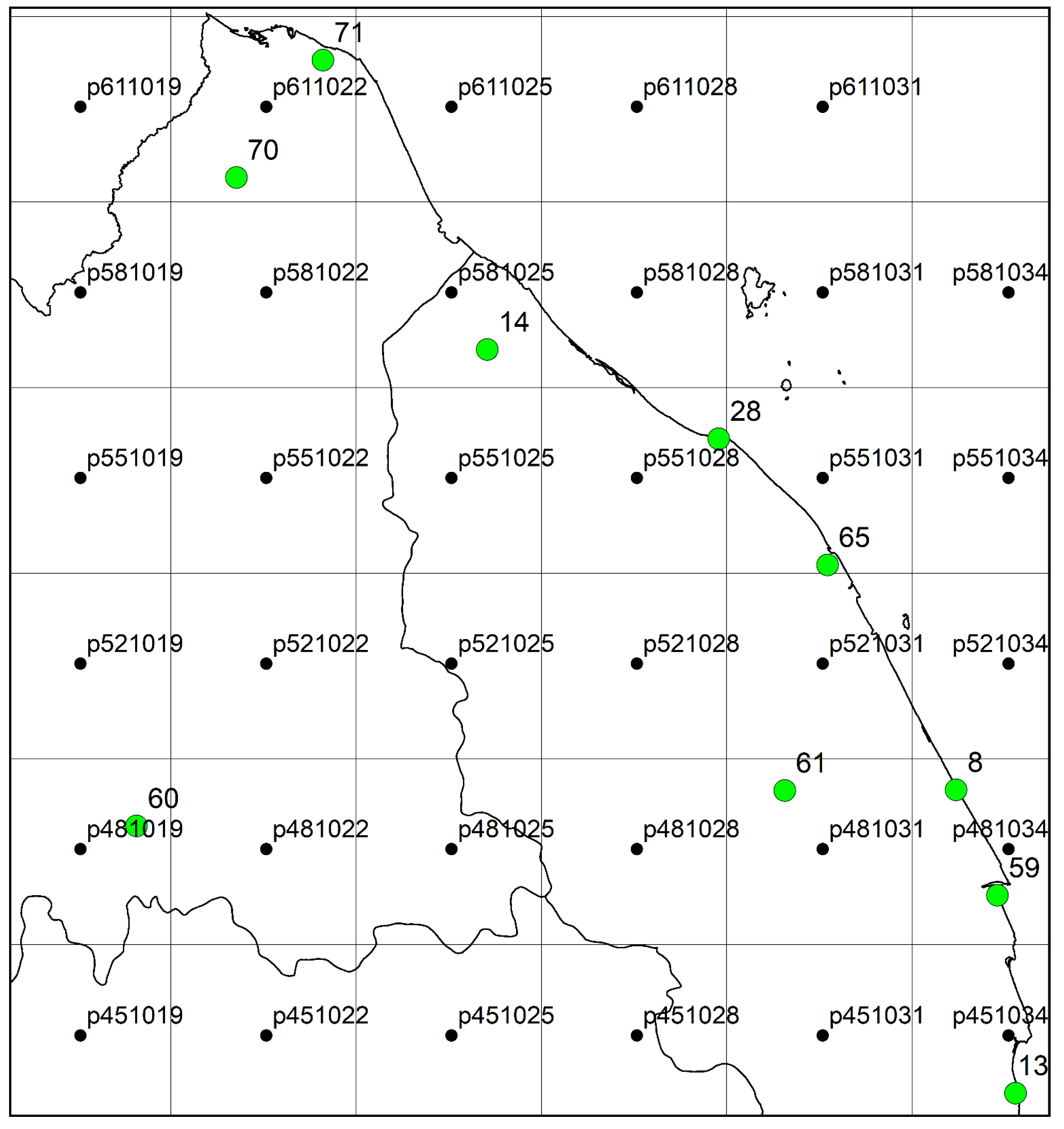
2.1. Study Area

Peninsular Malaysia lies in the equatorial zones of northern latitude between 1° and 7° N and eastern longitude from 100° to 103° E. The weather in Peninsular Malaysia is hot and humid all year. Generally, the climate in Malaysia is influenced by winds blowing from the Indian Ocean known as the southwest monsoon wind that occur from May to September, and winds blowing from the South China Sea known as the northeast monsoon wind, occurring from November to March. The study focuses on Peninsular Malaysia’s Kelantan and Terengganu states, located on the east coast of Peninsular Malaysia. As shown in Figure 1, the green dots represent stations of observation of rainfall on the ground, while the black dots represent those of atmospheric observation. The atmospheric stations are represented in the grid scale. For the case study, 10 rainfall observation stations located across east-coast Peninsular Malaysia were chosen. Conversely, the eight stations were chosen based on their proximity to the nearest atmospheric grid. For example, if two ground stations (codes 70 and 71) shared the same atmospheric station, the ground station closest to the atmospheric grid that is code 71 was chosen. The details of selected stations is shown in

Table 1. Geographical coordinates of nine match stations in east-coast Peninsular Malaysia between rainfall and atmospheric stations.

No.	Code of Atmospheric Station	Code of Ground Station	Name of Ground Station	Longitude	Latitude
1	P611022	71	Kota Bharu	102.28	6.17
2	P551028	28	Kg Merang, Setiu	102.29	5.68
3	P581025	14	Sek. Keb, Kg Jabi	102.56	5.68
4	P551031	65	Stor JPS Kuala Terengganu	103.13	5.32
5	P481019	60	Gua Musang	101.97	4.88
6	P481031	61	Kg. Menerong	103.06	4.94
7	P481034	59	Sek. Men. Sultan Omar, Dungun	103.42	4.76
8	P451034	13	Sek. Keb. Kemasek	103.45	4.43

.

2.2. Predictor and Predictand

The data used in this study include atmospheric data (predictors) and daily rainfall data (predictands) at selected stations stated in Table 1. Daily rainfall data series from 1998 to 2007 were obtained from the Department of Irrigation and Drainage (DID). The total number of daily rainfall measurements without missing values is 32,869, and the unit of daily rainfall is listed as millimetres per day (mm/day), which is the depth of rainwater (mm) accumulated in a 24 h period (day). The descriptive statistics of predictand data were represented by the mean of data being 7.39, the standard deviation being 20.45, the skewness of data being 6.45 and the kurtosis of data being 62.64. The result of skewness illustrates that the shape of predictand distribution for nine stations is positively skewed and indicates that the value of mean is more than median. Moreover, the value of kurtosis shows the data have a heavier tail compared to the tail of a normal distribution.

In this study, the large-scale atmospheric variables from the National Centers of Environment Prediction (NCEP) Climate Forecast System Reanalysis (CFSR) dataset are candidates for predictors. A set of six large-scale atmospheric variables was converted by using Fishnet Polygon and the list of predictors is shown in

Table 2. The six large-scale atmospheric reanalysis NCEP-CFSR variables.

Variable	Unit	Mean	Standard Deviation	Skewness	Kurtosis
Minimum temperature	°C	30.05	2.71	−0.05	0.36
Maximum temperature	°C	22.33	2.21	−0.05	0.24
Precipitation	mm	9.49	14.03	5.12	44.94
Wind	knot	1.52	0.80	2.10	6.49
Relative humidity	%	0.83	0.08	−0.39	−0.35
Solar	W/m2	20.37	5.93	−1.26	1.04

. Additionally, Table 2 also includes the descriptive statistics such as mean, standard deviation, skewness and kurtosis of predictor data. The predictor data employed in this study gathered a total of 27,470 days and 5.5% of missing values.

Section 2.3 delves into the theory behind all of the models used in this study and Section 2.4 details the application of all techniques in development of statistical downscaling model.

2.3. Theory of Models Used

2.3.1. Random Forest (RF)

RF is a generalization algorithm for Decision Tree ensembles that uses bagging to combine different random predictors in order to gather predictors [28]. They accommodate complexity while avoiding over-generalization of the training data [29]. Breiman [30] introduced RF, which can be used for classification and regression and has been used in the context of missing data.

Let us assume that dataset $X=X_1, X_2, X_3,\dots ,X_p$ is an $n\times p$ dimensional data matrix. Moreover, $X_s$ contains all the missing values at entries $i_{miss}^{\left(s\right)}\subseteq \left\{1,\dots ,n\right\}$. Then, the imputation approach should be repeated until a stopping criterion is reached. The stopping criterion $\left(\gamma \right)$ is met when the difference between the last imputed data matrix and the previous data increases for the first time, with respect to each variable. Differences for the set of continuously varying variables, $N$ is defined as

$${\Delta }_N=\frac{{{\displaystyle \sum }}_{j\in N}{\left(x_{new}^{imp}-x_{old}^{imp}\right)}^2}{{{\displaystyle \sum }}_{j\in N}{\left(x_{new}^{imp}\right)}^2}$$

(1)

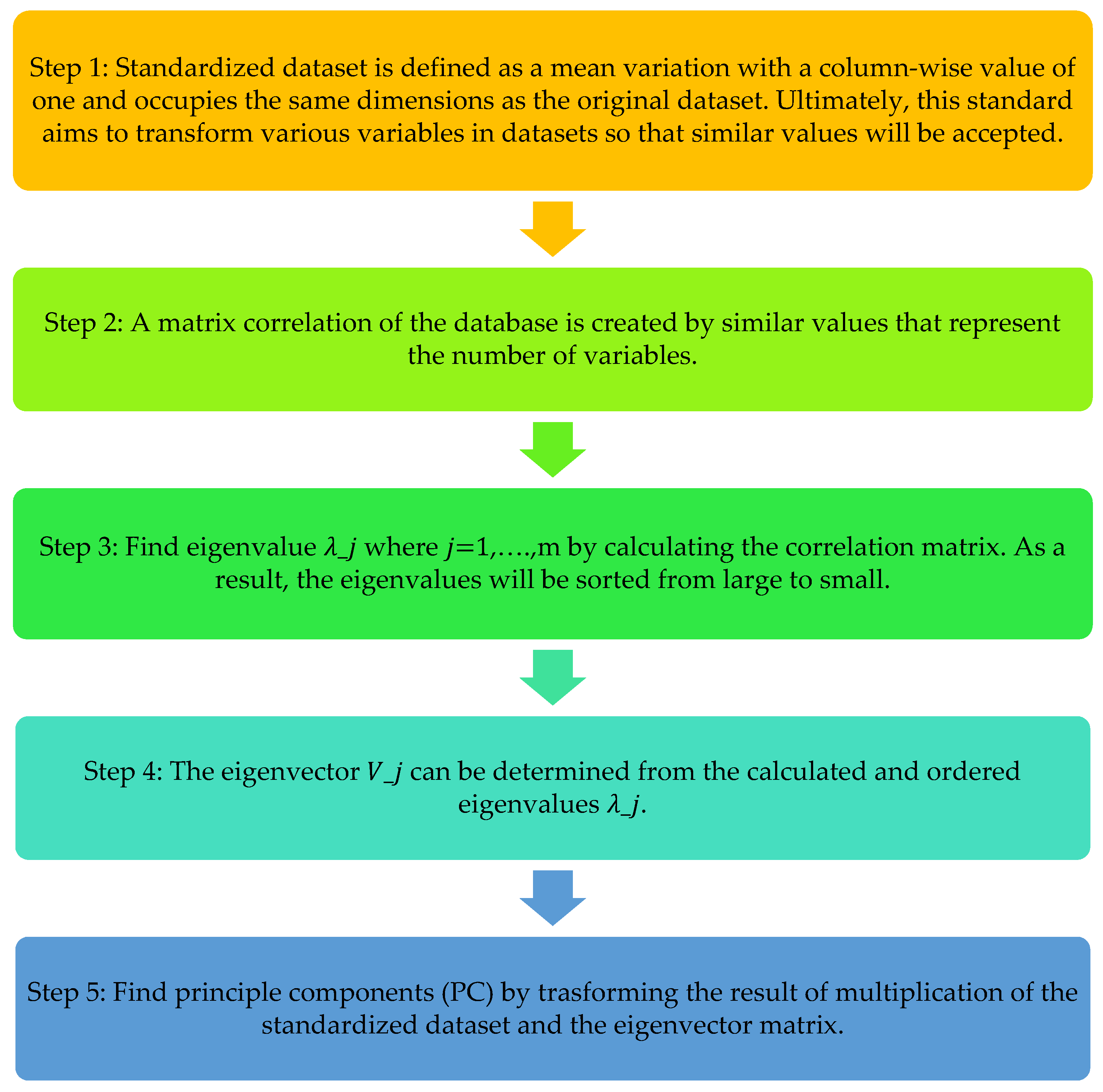
2.3.2. Principal Component Analysis (PCA)

In many fields, such as hydrology, geography, agriculture and others, large datasets are becoming more popular. To interpret such datasets, methods must drastically reduce their dimensionalities in an interpretable manner by preserving the majority of the data’s information. PCA is one of the oldest and most widely used techniques for developing large dataset studies [31]. The standard context for PCA as data analysis technique is by a set of data with observation on $p$ variables for each $n$ entities. Moreover, $X$ is an $n\times p$ data matrix. A classical PCA is applied to a $p\times p$ correlation matrix and calculated as follows:

$$M={\left(n-1\right)}^{-1}{S}^{T}S$$

(2)

where $S$ is a standardized dataset and $T$ stands for transpose. Then the eigenvalues ${\lambda }_j$ for the correlation matrix are determined as follows:

$$Me=\lambda e$$

(3)

where $e$ is linear weight that defines each loading for principal component (PC). Moreover, the eigenvectors $V_j$ are determined by calculating and ordering the eigenvalues ${\lambda }_{sj}$ of correlation matrix, $M$.

$$\left(M-{\lambda }_{sj}\times \mathrm{I}\right)\times V_j=0$$

(4)

Furthermore, lastly the subsequent multiplication of standardized data $S$ with eigenvector matrix $V=V_j$ results in the transformed dataset PC. Since $M$ is a correlation matrix, it is symmetric, and linear algebra dictates that the eigenvectors must be orthogonal. The symmetric correlation matrix is a positive matrix; thus, the given eigenvector is always $\ge 0$.

2.3.3. Support Vector Machine (SVM)

Support Vector Machine (SVM) is a powerful machine learning tool proposed by [32] that has attracted the attention of machine learning researchers and the community. SVM is a kernel-based function that can be applied to both linear and nonlinear analysis [33]. SVM can be used for classifying and predicting, and it is called Support Vector Classification (SVC) for classification and Support Vector Regression (SVR) for predicting. SVMs can handle high-dimensional data very well and they can predict with high degrees of accuracy in classification [34]. However, the challenge of using them is determining the best penalty term parameter and kernel parameters. This is because SVM is very sensitive to the parameter used. In [35], there is a review of use of SVM in hydrology.

Support Vector Classification (SVC)

Consider that dataset from PCs is divided into two sets, which are training data and testing data. The training data have two classes [($x_1,y_1),\left(x_2,y_2\right),\dots \dots ,\left(x_i,y_i\right)$], and the input vector is $x_i$ and the output is $y_i$. The output is labelled by $y_iϵ\left\{+1,-1\right\}$. The classifier for the problem of binary classification is

$$f\left(x\right)=sign\left[w^T\times \varphi \left(x\right)+b\right]$$

(5)

where the input vector $\left(x\right)$ is mapped with a feature space by nonlinear function $\varphi \left(x\right)$. Then, $w$ and $b$ are the classifier parameters. Optimization problems can be solved by determining the SVM classifier from theory as shown below

$$\begin{gathered} \min \hspace{1em}\hspace{1em}\frac{1}{2}{w}^T\times w+C{\displaystyle \sum }_{i=1}^l{\xi }_i \\ \mathrm{subject}\mathrm{to} y_i\left[w^T\times \varphi \left(x_i\right)+b\right]\ge 1-{\xi }_i \\ {\xi }_i\ge 0, i=1,\dots .,l \end{gathered}$$

(6)

where ${\xi }_i$ is a non-negative slack variable that influences objective function when data are misclassified. Then, $C$ is a penalty parameter with positive value. The optimization problems are solved by using Lagrange multiple ${\alpha }_i$, where $0 \le {\alpha }_i\le C$. Hence, the classifier in Equation (6) will be a series of mathematical derivation.

$$f\left(x\right)=sign({\displaystyle \sum }_{ij=1}^l{\alpha }_i{y}_i\varphi {\left(x_i\right)}^T\times \varphi \left(x_j\right)+b$$

(7)

The kernel function, $K\left(x_i,x_j\right)=\varphi {(x_i)}^T\times \varphi \left(x_j\right)$, is used to calculate the inner products. In SVM classification, there are a few possible kernels, but the common ones are linear, polynomial, radial basis function and sigmoid. It is likely that the radial basis function with parameter $\gamma$ will be the most popular and capable kernel.

$$K(x,x^{\text{'}})=\{\begin{array}{c}{x}^T\times x^{\prime } linear\\ {\left(x^T\times x^{\prime }+1\right)}^d polynomial\\ \exp (-\gamma |\left|x-x^{\prime }\right|{|}^2) RBF \\ \tanh \left(\gamma x\times x^{\prime }+C\right) sigmoid \end{array}$$

(8)

In the final classifier, only nonzero Lagrange multiples will take part as indicated in Equation (7). The data which have nonzero corresponding Lagrange multiples will be named as support vectors. Then, the classifier will be written as

$$f\left(x\right)=sign({\displaystyle \sum }_{k=1}^m{\alpha }_k{y}_{k}K\left(x_k,x\right)+b)$$

(9)

where $x_k$ is the support vector and $m$is the number of support vectors. In the support vector classifier, there are two parameters to calibrate which are $C$ (penalty term) and $\gamma$ (gamma). Those parameters are needed to satisfy the classifier algorithm in Equation (9).

Support Vector Regression (SVR)

Datasets from PCs are divided into two types: training data and testing data. The training data have two classes [$(x_1,y_1),\left(x_2,y_2\right),\dots \dots ,\left(x_i,y_i\right)$], and the input vector is $x_i$ and the output is $y_i$. The output is labelled by $y_iϵ\left\{R^m\times R\right\}$. In Support Vector Regression, the original data are mapped to a new feature space by using function of $\phi .$ Likewise, linear machine learning can also be used to discover nonlinear machine learning [36]. The regression prediction function can be expressed as:

$$f\left(x\right)=w^T\phi \left(x_i\right)+b$$

(10)

where $w$and $b$ can be obtained by finding the solution of the following optimization problem:

$$\begin{gathered} \min \frac{1 }{2}{\left|\left|w\right|\right|}^2+C{\displaystyle \sum }_{i=1}^l\left({\xi }_i+{\xi }_i{}^{*}\right) \\ \mathrm{Subject}\mathrm{to}(\langle w^t\varnothing \left(x_i\right)\rangle +b)-y_i\le \epsilon +{\xi }_i \\ (\langle w^t\varnothing \left(x_i\right)\rangle +b)-y_i\le \epsilon +{\xi }_i{}^{*} \\ {\xi }_i,{\xi }_i{}^{*}\ge 0 \left(i=1,2,\dots ,n\right) \end{gathered}$$

(11)

In Equation (11), the first item makes the function plainer and helps improve generalization [37]. The $C$ parameter, called penalty term, expresses the penalty for an experiential error. When $C$ is a small value, the penalty for experiential error is small and then results in less fitting and predicting errors. Moreover, if the $C$ is large, the penalty for experiential error will be extra-large, which will lead to over-learning.

Based on Equation (11), $\epsilon$ represents the nonsensitive loss function with positive constant. If the difference between the predictive value $f\left(x\right)$ and the real value $y_i$ is less than value of $\epsilon$, it is ignored. However, if the error difference is more than $\epsilon$, the error will be $\left|f\left(x_i\right)-y_i\right|-\epsilon$. The $\epsilon$ indicates the expectation of an error between the predictive value and real value. If the value of $\epsilon$ is less than the demand, the error will be less but there will be higher prediction precision.

By introducing Lagrange function and kernel function, the problem regrading nonlinear data is able to simplify. Equation (11) was transformed into the following quadratic function maximizing problem as follows:

$$\begin{gathered} \max {\displaystyle \sum }_{i=1}^l\left({\alpha }_i{}^{*}+{\alpha }_i\right)y_i-\epsilon {\displaystyle \sum }_{i=1}^l\left({\alpha }_i{}^{*}+{\alpha }_i\right) \\ -\frac{1}{2}{\displaystyle \sum }_{i,j=1}^l\left({\alpha }_i{}^{*}-{\alpha }_i\right)\left({\alpha }_j{}^{*}-{\alpha }_j\right)K\left(x_i,x_j\right) \\ \mathrm{Subject}\mathrm{to}0\le {\alpha }_i, {\alpha }_i{}^{*}\le C \left(i=1,2,\dots ,n\right) \\ {\displaystyle \sum }_{i=1}^l({\alpha }_i{}^{*}-{\alpha }_i{}^{*})=0 \end{gathered}$$

(12)

Therefore, the final prediction function will be

$$f\left(x,{\alpha }_i,{\alpha }_i{}^{*}\right)={\displaystyle \sum }_{i=1}^l\left({\alpha }_i-{\alpha }_i{}^{*}\right)K\left(x_i,x\right)+b$$

(13)

In Equations (12) and (13), the function of $K\left(x_i,x\right)$ represents kernel function. The kernel function, $K\left(x_i,x_j\right)=\varphi {(x_i)}^T\times \varphi \left(x_j\right)$, was introduced to calculate the inner products. Based on each kernel type’s algorithm in Equation (8), $\sigma$ is kernel parameter gamma. A large number of experiments have shown that the value of gamma influences the performance SVM model seriously [36]. A high value of gamma will reduce the structural risk and make more slippery the function curve (at the same time maximizing the experiential error). In addition, an over-small gamma will result in an over-fitted model.

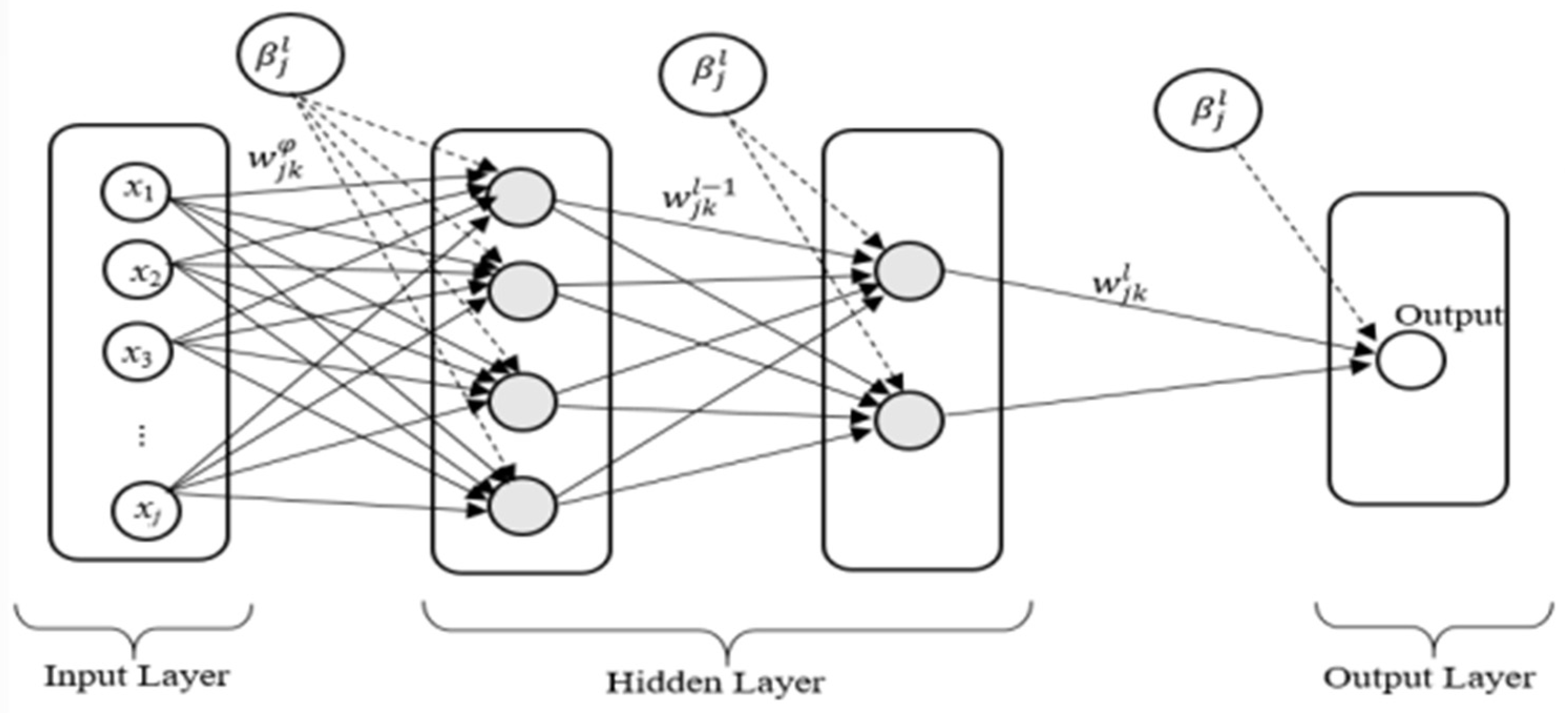
2.3.4. Artificial Neural Network (ANN)

Artificial Neural Network (ANN) is a technique that has been widely established to model complex nonlinear and dynamic systems. ANNs are useful in understanding an appropriate model when the physical process relationship is not clear or if the nature of the event has unstable properties [38]. In previous seasons, Artificial Neural Network (ANN) models have been commonly referred to as black box models that have been successfully used for modelling complex hydrological processes, such as rainfall-runoff, which have been shown to be viable tools in hydrology [39].

The learning process seeks to find a set of weights that gives a mapping that fits well with input and output. The following as an arbitrary nonlinear function could be assumed:

$$F\left(x,w\right)=y$$

(14)

where x represents the input vector (predictors) presented to network, $w$ is the weight of the network, $y$ is the corresponding output (predictand) which is approximated or predicted by the network. The number of neurons in the hidden layer is calculated as Equation (7).

$$l=\frac{1}{2}\left(i+o\right)+\sqrt{N}$$

(15)

where $l$ is number of nodes in hidden layer, $i$ is the number of input neurons and $o$ is the number of output neurons. $N$ is the number of records in the training set. The structure of ANN algorithm is as follows:

$${\widehat{y}}_k=f_o\left[{\displaystyle \sum }_{j=1}^l{\omega }_k{}_j\times f_h\left({\displaystyle \sum }_{i=1}^{N_n}{\omega }_{ji}{x}_i+{\omega }_j{}_o\right)+{\omega }_{k0}\right]$$

(16)

where ${\omega }_{ji}$ is the weight of the hidden layer, which connects the $i$th neuron in the input layer to the $j$th neuron in the hidden layer, and ${\omega }_k{}_j$ represents the $j$th neuron bias. The $f_h$ are the $j$th hidden neuron activation functions. In Equation (16), ${\omega }_j{}_o$ is the parameter of the output layer which connects the $j$th neuron in the hidden layer to the $k$th neuron in the output layer, and ${\omega }_{k0}$ is the bias for the $k$th output neuron. In addition, $f_o$ is the activation function for the output neuron, $x_i$ shows the $i$th input data and ${\widehat{y}}_k$ denotes the calculated output. Moreover, $N_n$ represents the number of neurons in input layers.

2.3.5. Relevance Vector Machine (RVM)

RVM is a variant of SVM because it is based on the same statistical learning framework as SVM. However, the study by [40] said that RVM has an additional functional algorithm based on probabilistic regression apart from its predecessor SVM. In RVM, a fully probabilistic concept is adopted and introduced a priori over the model weights, which are defined as a set of hyperparameters, and then is linked to weights, whose most likely values are iteratively predicted from the data [41].

Consider a set of data ${\left(x_i,y_i\right)}_{i=1}{}^n$, where $x_i$ are the input vectors and $y_i$ are the target vectors. The output of model is represented in Equation (17). Based on Equation (17), $w_i$ represents the vector of weight and $k\left(x,x_i\right)$ is kernel function. Then, ${\epsilon }_n$ is the bias that is assumed to be Gaussian with a mean of zero and a variance ${\sigma }^2$.

$$y\left(x\right)={\displaystyle \sum }_{i=1}^n{w}_{i}k\left(x,x_i\right)+{\epsilon }_n$$

(17)

The likelihood of the complete dataset can be expressed as

$$p\left(y|w,{\sigma }^2\right)={\left(2\pi {\sigma }^2\right)}^{-\frac{n}{2}}exp\left[-\frac{1}{2{\sigma }^2}{\left||y-\Phi |\right|}^2\right]$$

(18)

where $\Phi ={\left[1,k\left(x_i,x_1\right),k\left(x_i,x_2\right)\dots .k\left(x_i,x_n\right)\right]}^T$is a matrix $nx\left(n+1\right)$ in size, with ${\Phi }_{nm}=k\left(x_n,x_{m-1}\right)$ and ${\Phi }_{n1}=1$. The maximum likelihood estimations of $w$ and ${\sigma }^2$ often result in over-fitting. According to [40], prior constraints on the parameter can be obtained by adding complex penalty to likelihood or error functions. The ability of the learning process to generalize is governed by this prior information. Based on Equation (19), $\alpha$ is a vector of $\left(n+1\right)$ hyperparameters that is used to constrain an explicit zero-mean Gaussian prior probability distribution over the weights $w$ and controls each weight away from zero.

$$p\left(w|\alpha \right)={\displaystyle \prod }_{i=0}^{n}N(w_i|0,a_i{}^{-1})$$

(19)

Eventually, using the Bayesian rule, the posterior over all unknowns can be achieved given the defined noninformative prior distribution [40,42].

$$p\left(w,\alpha ,{\sigma }^2|y\right)=\frac{p\left(y|w,\alpha ,{\sigma }^2\right)\times p\left(w,\alpha ,{\sigma }^2\right)}{{\displaystyle \int }p\left(y|w,\alpha ,{\sigma }^2\right)p\left(w,\alpha ,{\sigma }^2\right)dwd\alpha d{\sigma }^2}$$

(20)

The direct solution in Equation (20) cannot be performed as the integral on the right-hand-side. As a solution for these issues, the posterior is decomposed as Equation (21),

$$p\left(w,\alpha ,{\sigma }^2|y\right)=p\left(w|y,\alpha ,{\sigma }^2\right)\times p\left(\alpha ,{\sigma }^2|y\right)$$

(21)

Furthermore, the posterior distribution of the weights can be expressed as Equation (22), where $\Sigma$ and $\mu$ are covariance and mean, respectively:

$$p\left(w|y,\alpha ,{\sigma }^2\right)=2{\pi }^{-\left(n+1\right)/2}{|\Sigma |}^{-1/2}\times exp\left\{-\frac{1}{2}{\left(w-\mu \right)}^T\times {\Sigma }^{-1}\left(w-\mu \right)\right\}$$

(22)

where the posterior covariance in Equation (23) and mean in Equation (24), respectively, are

$$\Sigma ={\left({\sigma }^2{\Phi }^2\Phi +A\right)}^{-1}$$

(23)

$$\mu ={\sigma }^{-2}\Sigma {\Phi }^{T}y$$

(24)

Moreover, the maximization of $p(y|\alpha ,{\sigma }^2)$ is required for uniform hyperpriors and achieved by Equation (25),

$$p\left(y|\alpha ,{\sigma }^2\right)={\displaystyle \int }p\left(y|w,{\sigma }^2\right)p\left(w|\alpha \right)dw$$

(25)

2.3.6. Evaluation Performance of Statistical Downscaling Model

This study evaluates the predicted output of the downscaling model using two types of evaluation performance. The measurements used in this study are Root Mean Square Error (RMSE) and Nash–Sutcliffe Efficiency (NSE), where the best model is selected based on the smallest value for RMSE. For the NSE, the efficiency index lies between 0 and 1 and approaching 1 indicates better performance of model. The equations for each of the evaluations’ performances are shown as follows:

$$\mathrm{RMSE}=\sqrt{\frac{{{\displaystyle \sum }}_{i=1}^N{\left(O_i-P_i\right)}^2}{N}}$$

(26)

$$\mathrm{NSE}=1-\frac{{{\displaystyle \sum }}_{i=1}^N{\left(O_i-P_i\right)}^2}{{{\displaystyle \sum }}_{i=1}^N{\left(O_i-\overline{O}\right)}^2}$$

(27)

where $O_i$ is observed data, $P_i$ denotes the prediction data, $N$ is amount of sample data and $\overline{O}$ is the mean of observed values.

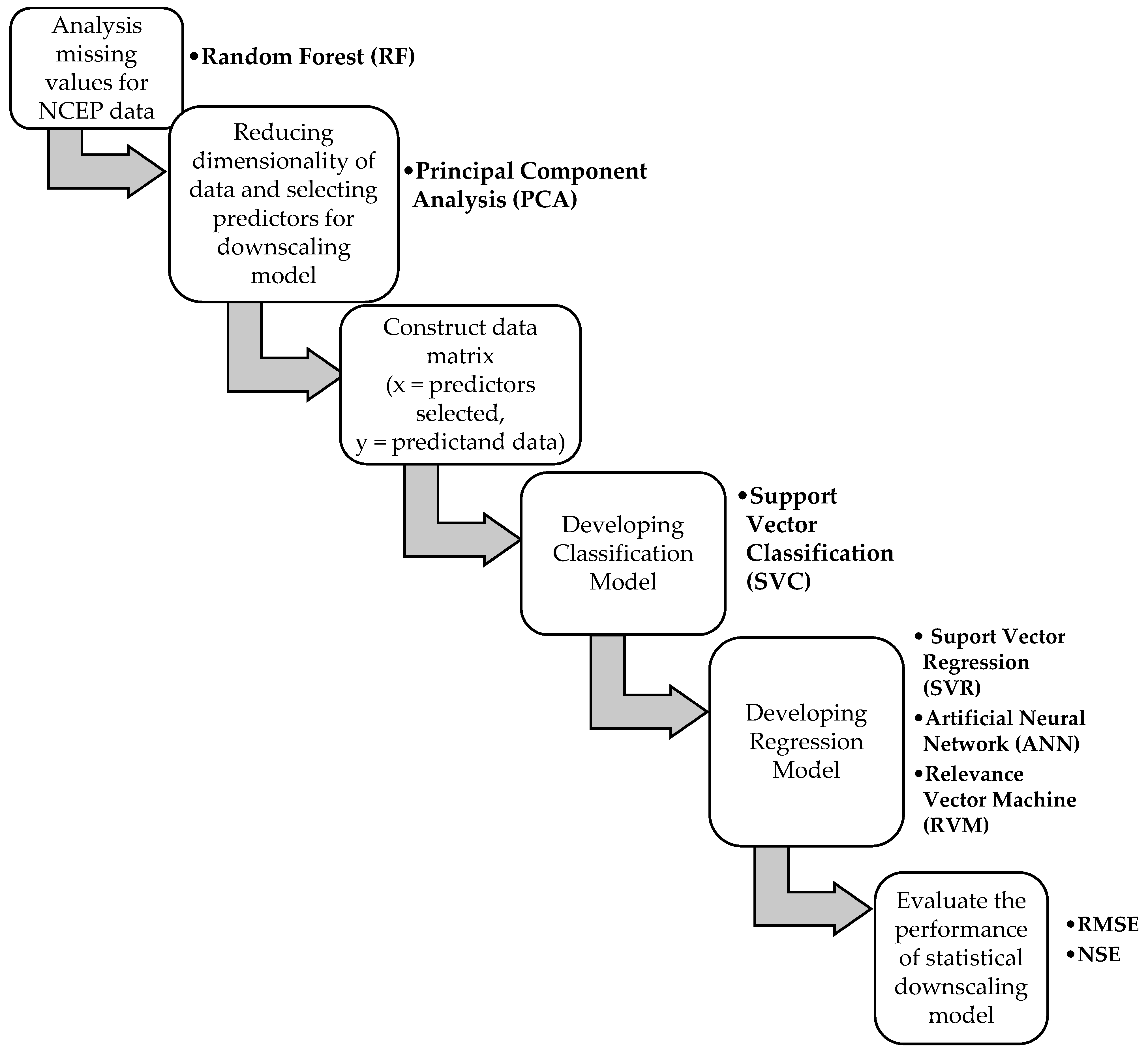
2.3.7. Flowchart of Statistical Downscaling Method

The proposed statistical downscaling method for daily rainfall consists of both classification and regression models, which were developed using machine learning techniques described in this section. The proposed model consists of data collection from predictors (atmospheric data) and predictands (rainfall data). As a preprocessing phase, the predictors were replenished by using RF. Then, PCA was used to select predictor variables while also reducing the data’s dimensionality. The new data matrices between the selected predictors and predictands were then created. Following that, a classification model was used to classify the days as dry or wet, in which a day with an amount of rainfall exceeding 1 mm is considered a wet day [14]. If the day is classified as a wet day, suitable regression techniques are used to predict the rainfall values. The proposed statistical downscaling model is shown in Figure 2.

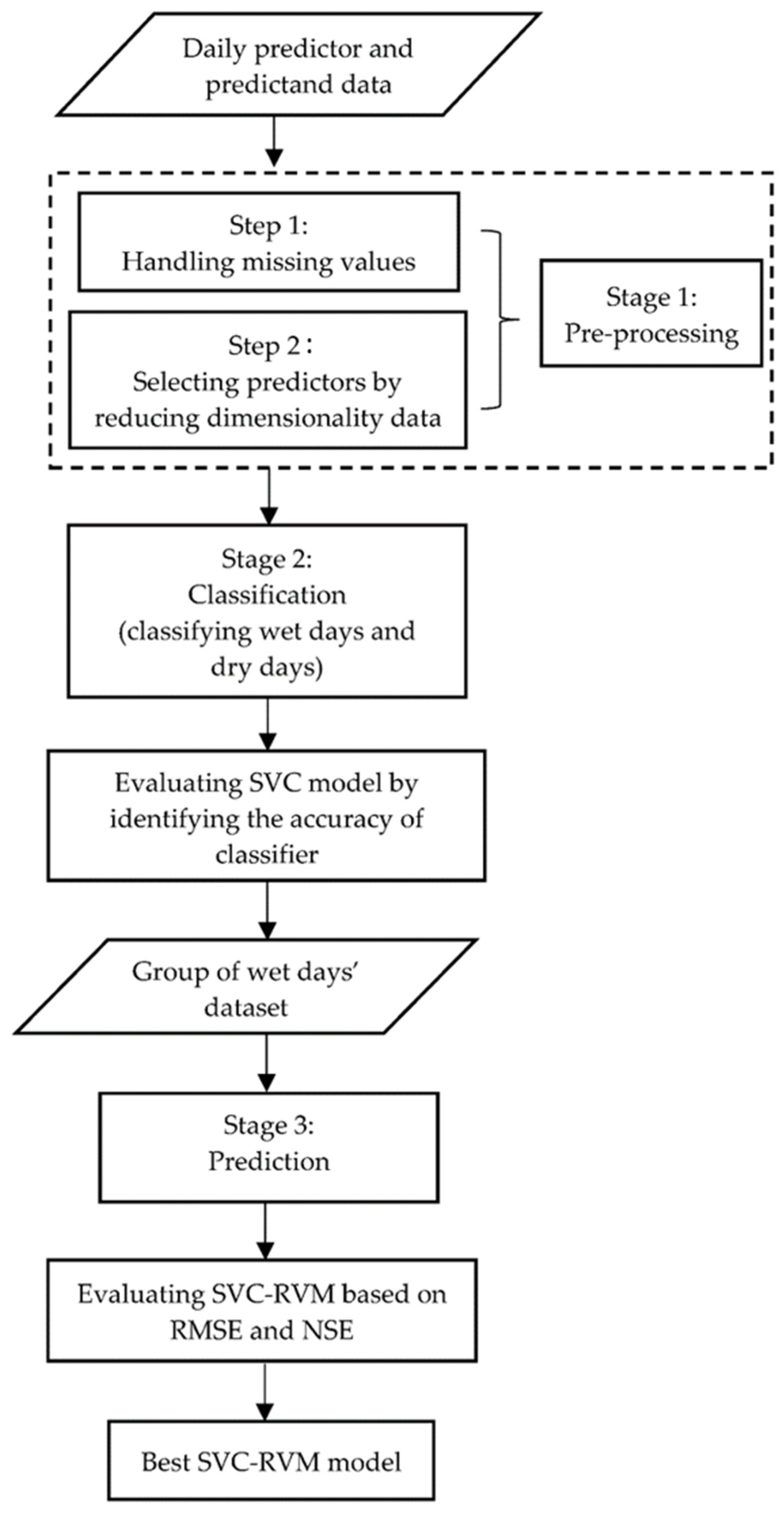
2.4. Procedure in Developing Statistical Downscaling Model

This subsection presents the application of the machine learning techniques detailed in Section 2.3 to develop statistical downscaling models for the nine rainfall stations in east-coast Peninsular Malaysia.

2.4.1. Pre-Processing Steps of Inputs in Statistical Downscaling Models

Analysis Missing Values of NCEP Data

The NCEP atmospheric data used in this statistical downscaling study range from 1998 to 2007. There are some missing data for each variable in predictors data. Before proceeding with the analysis, the mechanism and pattern of missing data must be identified. The analysis of missing values was conducted by using the RF model. The steps of RF are as follows:

(1)

Step 1: Initializing. The missing values will be replaced by the mean of data (continuous variables) or the most frequent class (categorical variables).

(2)

Step 2: Imputation. The imputation process is carried out consecutively for each variable in ascending or descending order of missing observations for each variable. The RF model is built using the variable under imputation as the response. The dataset’s observations are divided into two groups based on whether the variable was observed or missing in the original dataset. The training set is made up of observed observations, while the prediction set is made up of missing observations [43]. Predictions from RF models are used to fill in the missing part of the variable under imputation [44].

(3)

Step 3: Stop. One imputation iteration is completed when all variables with missing data have been imputed. MissForest outputs the previous imputation as the final result after iterating the imputation process until the relative sum of squared differences between the current and previous imputation results increases [45].

Reducing Dimensionality of Data and Selection of Predictors

High-dimensional data interfere with model performance by having the lowest accuracy of classification and the worst pattern recognition and visualization [46]. Moreover, the selection of predictors as input to statistical models is regarded as a critical task in any statistical downscaling study. PCA model was used in this study to assist in reducing the dimensionality of data and selecting variables of predictors. Principle component analysis (PCA) has two critical functions. It minimizes or reduces the number of variables and identifies principle components (PCs) which are linear combination of variables [47,48]. There are specific properties of PCs with respect to variance [27]. Figure 3 depicts the steps involved in PCA.

2.4.2. Development of Downscaling Model

Developing Classification Model

A classification model is then developed after the predictor selection. The proposed classification model is based on SVC. The algorithm on conducting SVC was introduced in this section. However, parameter discovery is required in SVC. Based on that, the parameter range was determined and examined in order to identify the best value of parameters ($C$, $\gamma$ and type of kernel) in the SVC model for this study. If a day is classified as dry, then the local daily rainfall is assumed to be zero. If a day is classified as wet, then the rainfall amount is estimated using regression model. The accuracy of SVC model was measured as follows:

$$\mathrm{Accuracy}:\frac{\widehat{A}|A+\widehat{B}|B}{A+B}\times 100$$

(28)

where A is the number of dry days while B is the number of wet days. $\widehat{A}|A$ indicates the number of dry days which are correctly classified as dry days and $\widehat{B}|B$ represents the number of wet days that are correctly classified as wet days.

Developing Regression Model

(a)

SVR-and-RVM-based Statistical Downscaling Model

In general, optimizing the value of the turning parameters in the algorithm improves the performance of SVR downscaling models [49]. For this purpose, some techniques of optimization parameters, such as genetic algorithm [50], Bayesian framework [51], grid search [52] and cross-validation method [53], have been used in previous studies.

In SVR, the cross-validation method is one of the most commonly used techniques for turning parameter optimization [37]. Hence, the cross-validation method was used to modify the values of turning parameter SVR in this study. Cross-validation is similar to the method of repeated random subsampling, but the sampling is done in such a way that no two steps overlap [54]. In k-fold cross-validation, the sample data are split into K disjoint subsets $t_h\left(h=1, 2, 3,\dots ,K\right)$ of equal size [55]. The term of “fold” represents the number of resulting subsets. The model is trained by $K$ times, but only the omitted subsets are utilized to compute the prediction error. The model is trained using k − 1 subsets, which both represent the training set. Then, the model is applied to the remaining subset (validation set) and the performance is measured.

Furthermore, the performance of SVR and RVM models depends on the type of kernel function selected. The kernel function in the SVR and RVM algorithms maps a nonlinear problem into a linear problem in a multidimensional space [7]. Hence, choosing an appropriate kernel function is essential when using SVR and RVM algorithms [56]. The study by [57] also stated that the performance of model is highly dependent on the kernel function. In this study, the radial basis function (RBF) as well as polynomial, linear and sigmoid kernel functions were tested with SVR and RBF; and polynomial, Laplace, hyperbolic tangent, Bessel and ANOVA kernel functions were examined with RVM algorithm, in order to identify the best kernel function for statistical downscaling. The SVM-and-RVM-based statistical downscaling model which displayed the smallest RMSE was selected as the best type of kernel.

• (b) ANN-based statistical downscaling model

In this study, the multilayer feed-forward neural network (FFNN) algorithm [58] was used to develop statistical downscaling models for each station in east-coast Peninsular Malaysia. Most hydrology studies in the past have been performed using only one or two hidden layers [59]. In addition, according to [60], the hyperbolic tangent sigmoid activation function was widely used in previous studies for constructing ANN-based regression models.

The ANN uses a mathematical simulation approach that adopts a biological system to process the information that has been acquired and to drag outputs that have been properly trained for pattern recognition. The ANN used in this study is a three-layer learning network that consists of an input layer, a hidden layer and an output layer where weights are linked to each layer as in Figure 4. The input transmits the input signal values to the unprocessed nodes in hidden layer. The values are scattered to all the nodes in the hidden layer, depending on the connection weights.

As shown in Figure 4, it is a feed-forward propagation algorithm where $x_j$ is the input variable of the input layer with $j=1,\dots ,n$. There are kth neuron node columns, a row of jth neuron nodes and $w_{jk}^{\phi }$ weight for each input layer. The weights of first hidden layer are represented as $w_{jk}^{l-1}$ and $w_{jk}^1$, and $l-1$ is represented as second hidden layer. ${\beta }_j^l$ is the weight of bias vector in each neuron in the lth layer.

2.4.3. Hybrid Model of SVC-RVM

The new proposed statistical downscaling model based on machine learning techniques is the hybridization model from the combination of the SVC and RVM models. In this study, the SVC model is used as a classification model because it can work relatively well with a clear margin of separation between classes [61]. The hyperplane was created in the space with the greatest minimum distance margin between training samples belonging to different groups. The main advantage of using SVC as a classification model is that it only uses the training sample of the edge of the margin to separate classes rather than using class mean differences [62]. Then, the SVC model classified rainfall day characteristics into two categories, which are wet and dry days. Furthermore, the group of wet days was analysed by applying RVM as a regression model to identify the prediction of rainfall in east-coast Peninsular Malaysia. RVM is a probabilistic prediction method that uses any kernel function without requiring the regularization parameter to be set due to its ability to use non-Mercer kernels [63]. As the prediction model, RVM could reduce the sparsity in regression that could improve the generalization model while reducing the computational complexity [64]. Therefore, the hybrid model of SVC-RVM as statistical downscaling model based on machine learning techniques can contribute to the future rainfall predictions in east-coast Peninsular Malaysia. The flowchart of the developed hybrid model of SVC-RVM is illustrated in Figure 5.

3. Results

3.1. Results of Pre-Processing Inputs in Statistical Downscaling Model

3.1.1. Analysis of Missing Values of NCEP Data

The 27,470 daily predictors data from NCEP-CFSR for a time interval of over 10 years contain 5.5% missing values. In this study, the mechanism of missing values was determined using a heatmap by finding the correlation between the present and missing predictor variable values. Based on the review of previous rainfall and time series studies in [65,66], the mechanism of missing values always occurs, either known as MCAR or MAR, due to the occurrence of missingness independent of the other missing data and between the variables. Figure 6 presents the visualization correlation plot between missing and nonmissing data for predictors in east-coast Peninsular Malaysia. On the left and top axes are the variables on each ground station, where 1, 2, 3 and so on indicate the name of ground station as stated in Table 1. It should be noted that the scale on the right represents the correlation coefficient between predictors variables. The dark blue colour shows that the correlation value between predictor variables is 1.0, indicating a strong correlation, while the white colour represents no correlation between predictor variables. Hence, the visualization plot clearly shows that the mechanism of missing data for this study is classified as MCAR, where missingness is independent of other variables.

Following the identification of the characteristics of the missing data mechanisms, the missing analysis was carried out. The imputation methods, namely RF, were implemented to deal with the missing data challenge. The performance of the model was measured by two performance indicators: Root Mean Square Error (RMSE) and Nash–Sutcliffe Error (NSE). The results were generated based on the type of variables because of the possibility of differences in the relative method performance across datasets. The best model performance is indicated by the lowest RMSE values, which means that the difference between the estimated and observed values is small. Meanwhile, NSE values with a range of 0 to 1 indicate the model with good predictive skill [66]. The values of RMSE and NSE are represented in

Table 3. RMSE and NSE value of each variable’s predictors.

	Max. Temperature	Min. Temperature	Precipitation	Wind	Relative Humidity	Solar
RMSE	0.23	0.19	2.25	0.06	0.01	0.74
NSE	0.99	0.97	0.97	0.99	0.99	0.98

. According to Table 3, the RMSE of the RF is small for all variables in the predictors, thus making the RF able to fill in the missing data in the predictor dataset.

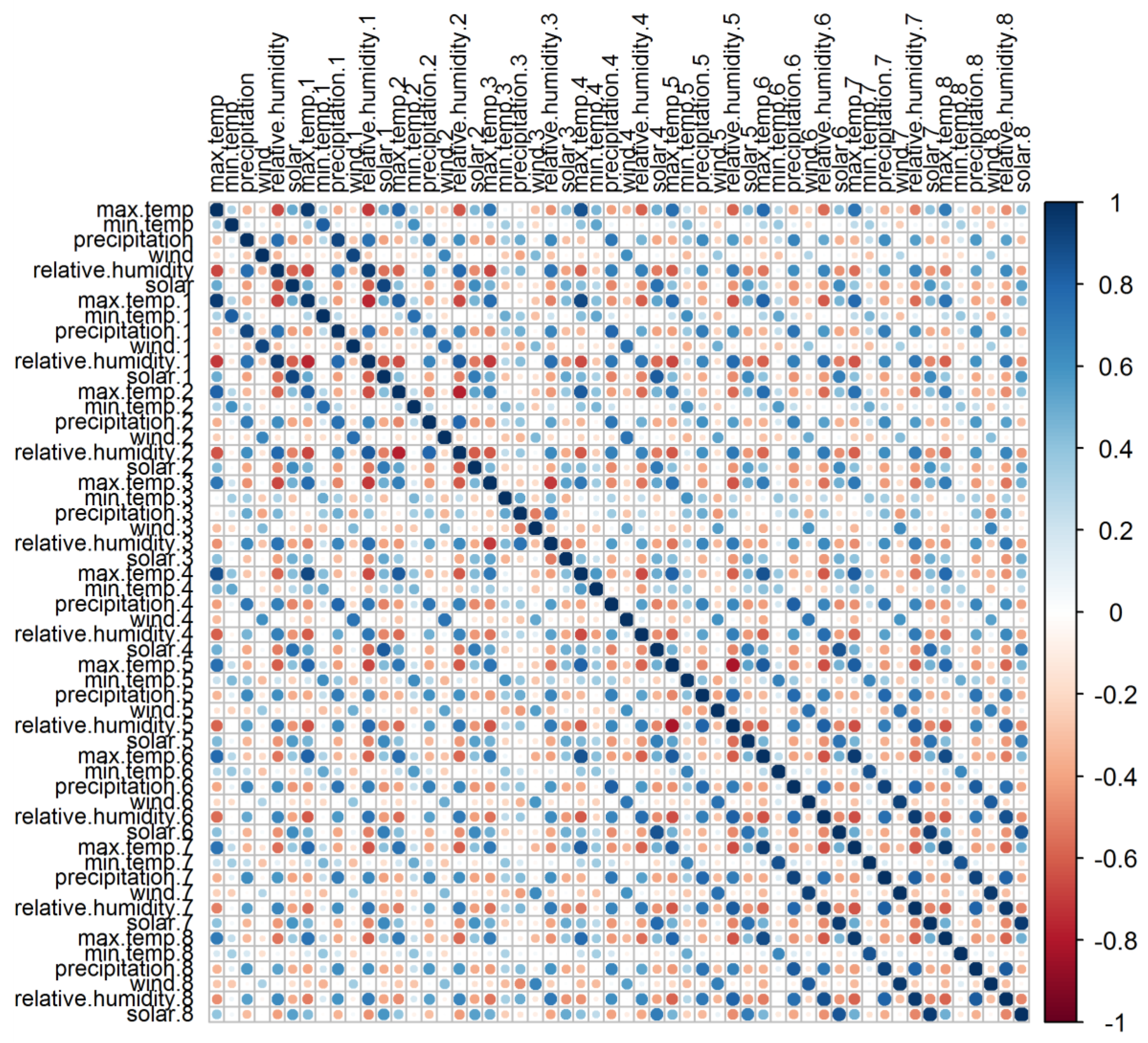
3.1.2. Reducing Dimension Data and Selection of Predictors

In the stage of reducing high-dimensional data, PCA was used as a dimension reduction approach to reduce the number of predictors by extracting the number of principal components (PCs) without losing any significant information. The results of the analysis include the eigenvalue, variation and cumulative percentage of variation, as presented in

Table 4. Results of Principal Component Analysis.

Dimension	Eigenvalue	Percent Variance	Cumulative Percentage
Component 1	2.62	43.66	43.66
Component 2	1.60	26.63	70.29
Component 3	0.64	10.63	80.92
Component 4	0.55	9.22	90.14
Component 5	0.45	7.53	97.68
Component 6	0.14	2.33	100.00

.

The analysis results in Table 4 show that six components were extracted based on the eigenvalues and total variation. The number of components produced in PCA was usually equivalent to the number of variables selected. The percentages of variation and eigenvalues were shown in decreasing order. The first component calculated has the greater eigenvalue and most percentage of variation. This is followed by the second component that accounts for most variation without accounting for the first component. The analysis continues until the overall variance in data is accounted for. However, based on the Kaiser criterion [67], eigenvalues of more than 1.00 were selected to interpret the component. Then, the results show Components 1 and 2 having eigenvalues of more than 1.00, which are 2.62 and 1.60, respectively. The significance of the two components also explains 70.29% of the total variance. According to [14], the best range to cut off the cumulative percentage of variation is higher than 70% for hydrological data.

Furthermore, PCA also can identify the factor with a significant influence on each variable. The projection of the original variables on the PC subspace that coincides with the alternation coefficients between the PCs and variables is called loading [68]. In PCA, the PCs are recommended to rotate for interpreting the relationship between PCs and the original variables easily [69]. According to the study by [70], significant PC loading is considered ‘weak’ when the component coefficients have a correlation of 0.49–0.30, ‘moderate’ when the coefficients have a correlation of 0.74–0.50 and ‘strong’ when the coefficients have a correlation of more than 0.75 (>0.75). Thus, PC loadings of more than 0.74, both positive and negative, were considered in this study.

Hence,

Table 5. Result of loading of each of the variables.

Predictors	Factor 1	Factor 2
Maximum temperature	0.85 *	−0.19
Minimum temperature	0.09	0.81 *
Precipitation	−0.75 *	0.20
Wind	−0.03	0.89 *
Relative humidity	0.86 *	0.28
Solar	0.79 *	0.01

* indicate the best results.

displays the correlation of the principal component (PC) loading of each variable of the predictors and factors generated. The number of factors generated was measured by the selected eigenvalues [70] in Table 4. Based on Table 5, Factor 1 has a strong positive loading on maximum temperature (0.85), relative humidity (0.86) and solar (0.79), while having a strong negative loading on precipitation (−0.75). The second factor shows strong positive loading for minimum temperature and wind. This finding is expected because such factors were extracted sequentially, where each factor accounted for as much of the remaining variance as possible [70]. Hence, all variables from NCEP-CFSR were selected as predictors for further analysis due to their high correlations based on the component loadings extracted from Factor 1 and Factor 2. Therefore, the new dataset was created in a matrix format: 32,869 rows representing the number of days by station and two columns known as Factor 1 and Factor 2 representing the factors extracted.

3.2. Results of Support Vector Classification in Predicting Categorical Rainfall Data

The new dataset formed by the PCA was replaced as an input into the classification model by Support Vector Classification (SVC). Through this study, the predictand data were converted based on attributes 0 and 1 for daily rainfall amount. The number of wet days in Peninsular Malaysia is defined as days with more than 1 mm of rainfall [14]. This study clarifies the wet days (>1 mm) as 1 and dry days, which have less than 1 mm of rainfall (<1 mm), are classified as 0. The performance of the SVC model depends on the selected value of parameters, which are penalty term, C, and type of kernel. Typically, SVC has four basic kernels known as radial basis, sigmoid, polynomial and linear functions [71].

Table 6. Summarized results of SVC.

Type of Kernel	Parameter			Calibration			Validation
	$\mathit{C}$	$\mathit{\gamma }$	$\mathit{d}$	No. of Support Vectors	Misclassification Error	Accuracy (%)	Misclassification Error	Accuracy (%)
RBF	10,000	1.00	-	12,363 *	0.351 *	64.90 *	0.326 *	67.40 *
Sigmoid	10,000	1.00	-	446	0.468	53.25	0.467	53.30
Linear	10,000	-	-	12,036	0.359	64.12	0.356	64.40
Polynomial	10,000	1.0	1	13,075	0.356	64.40	0.354	64.60
	10,000	1.0	2	14,597	0.466	53.40	0.447	55.30
	10,000	1.0	3	14,653	0.473	52.70	0.431	53.10

* indicates the best model selected.

represents the summarized performance of SVC in terms of the number of support vectors, misclassification error and accuracy of the model in the calibration and validation periods. In general, the RBF kernel is composed primarily of high-accuracy values during the calibration and validation periods. Moreover, Table 6 shows that the highest accuracy in the validation period is 67.40%. The polynomial kernel, on the other hand, has the lowest accuracy, with 53.10% validation and 52.70% calibration. The results of an SVC model based on various types of kernels can be seen in [9]. Besides that, the number of support vectors represents the data that approach a hyperplane in classification [72]. It is measured by the number of support vectors, with the smallest value considering far points from a hyperplane and the highest value considering close points with a hyperplane. Furthermore, a misclassification error is a type of measurement error representing the classified data that do not provide a true response to the actual data [73]. This study generated misclassification errors between 0.31 and 0.49 for validation and between 0.35 until 0.51 for the calibration period. Hence, this study found that the SVC model with a radial basis function (RBF) kernel and a pair of parameters (10,000, 1) is the best classification model, yielding the highest-accuracy percentage while having the lowest misclassification errors in the validation and calibration periods.

3.3. Results of Developing Regression Model in Predicting Rainfall Data

Regression analysis enables us to understand the relationship between the value of the predictor corresponding to predictand variable change [74]. The relationship can be identified using machine-learning-based predictive modelling as introduced in this study. The machine learning models involved in this study are Support Vector Regression (SVR), Artificial Neural Network (ANN) and Relevant Vector Machine (RVM). In addition, the datasets in this study consist of a matrix form of Factor 1 and Factor 2 from PCA, as well as a group of wet days determined by SVC.

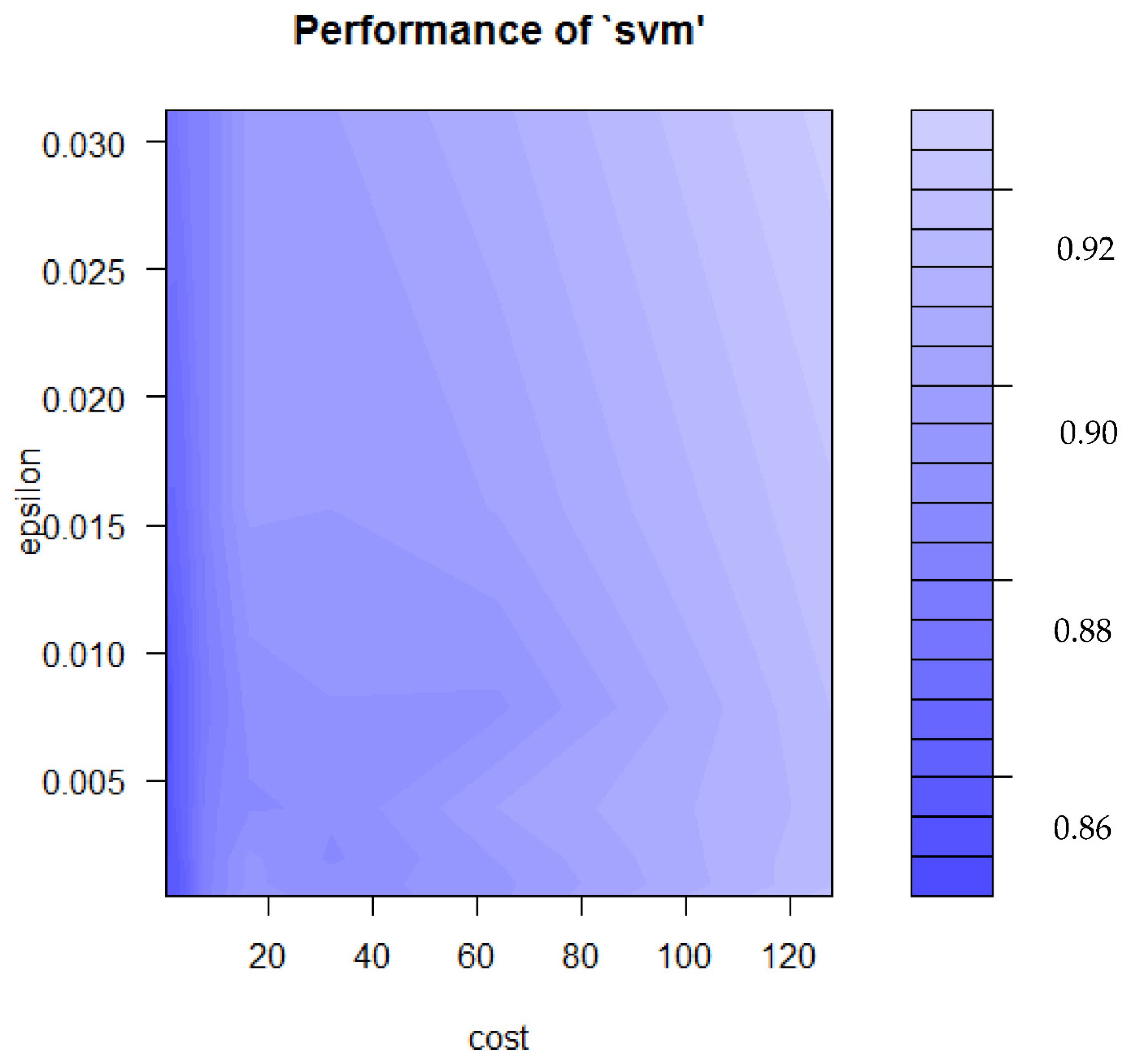
3.3.1. Results of Turning Parameters of SVR

In applying Support Vector Regression (SVR), the challenging task is deciding on the kernel type and selecting the gamma ($\gamma$), penalty terms ($C$) and epsilon ($\epsilon$) parameters. A previous study [75] stated that the performance of SVR is affected by the penalty terms $C$ and kernel function parameters. The authors of [76] found that the optimization process is required in SVM to prevent the over-fitting of the model. In this study, the method was applied to SVR to provide an optimization process, also known as turning, for the selection parameters of 10th-fold cross-validation (KCV). The range value of $C$ was tested in this study based on the previous study by [71].

Table 7. Results of optimization parameter $C$.

$\mathbf{Parameter}\mathit{C}$	RMSE
0.25	1.935
0.50 *	1.933 *
1.00	1.935
2.00	1.935
4.00	1.940
8.00	1.950
16.00	1.970
32.00	1.975
64.00	1.985
128.00	1.985

* indicates the selected value.

shows that the parameter $C$ performed the best at 0.5, while γ was constant at the value of 1.935. The model with the lowest RMSE value was chosen and will be used in the SVR for this study. After identifying $C$, the optimal value of $\epsilon$ was obtained, as shown in Figure 7. The range value of $\epsilon$ ($2^{-11}{,2}^{-10}{,2}^{-9}{,2}^{-8}{,2}^{-7}{,2}^{-6}{\mathrm{and}2}^{-5})$ was obtained from a study by [36]. Figure 7 presents the visualization of the turning parameters between $\epsilon$ and $C$. The blue scale on the right side represents the range of error estimation, where the darker the colour, the smaller the error produced. The error estimation was averaged over all $k$ trials to determine the total effectiveness of the SVR model [77]. Thus, the best value of $\epsilon$ is $2^{-10}$ by error, which is approaching 0.86. Therefore, the best set of parameters for the SVR model is $C$= 0.5, $\gamma$= 1.935 and $\epsilon$=$2^{-10}$.

3.3.2. Results of Selection of Kernel for RVM Model

In applying RVM as a regression model, identifying a selection of a specific kernel function is important because the model’s performance is dependent on it [56]. The selection of a kernel also improves the accuracy and sparsity result when optimizing the marginal likelihood respects to multiple input spaces in kernel functions [78]. Thus, this study aims to evaluate the RVM model through various types of kernels such as radial basis function (RBF), polynomial, Laplace, hyperbolic tangent, Bessel and ANOVA. The best performance of the kernel was determined through the value of the relevant vector and RMSE, as shown in

Table 8. Performance of RVM by different type of kernels.

Type of Kernel	Number of Relevant Vectors	RMSE
RBF	35	28.95
Polynomial	32	28.88
Laplace	15 *	19.75
Hyperbolic tangent	31	28.82
Bessel	34	28.93
ANOVA	38	29.0

* indicates the best kernel.

. RMSE is a good measure of how accurately the model predicts the response, and it is the most important fit criterion if the model’s primary purpose is prediction [79]. Then, the number of relevant vectors represents on the results of the Bayesian formulation, leading to sparser representation [80]. Hence, the Laplace kernel was chosen as the best RVM model because it produced the lowest value of RMSE, and in addition, the Laplace kernel resulted in the least number of relevant vectors.

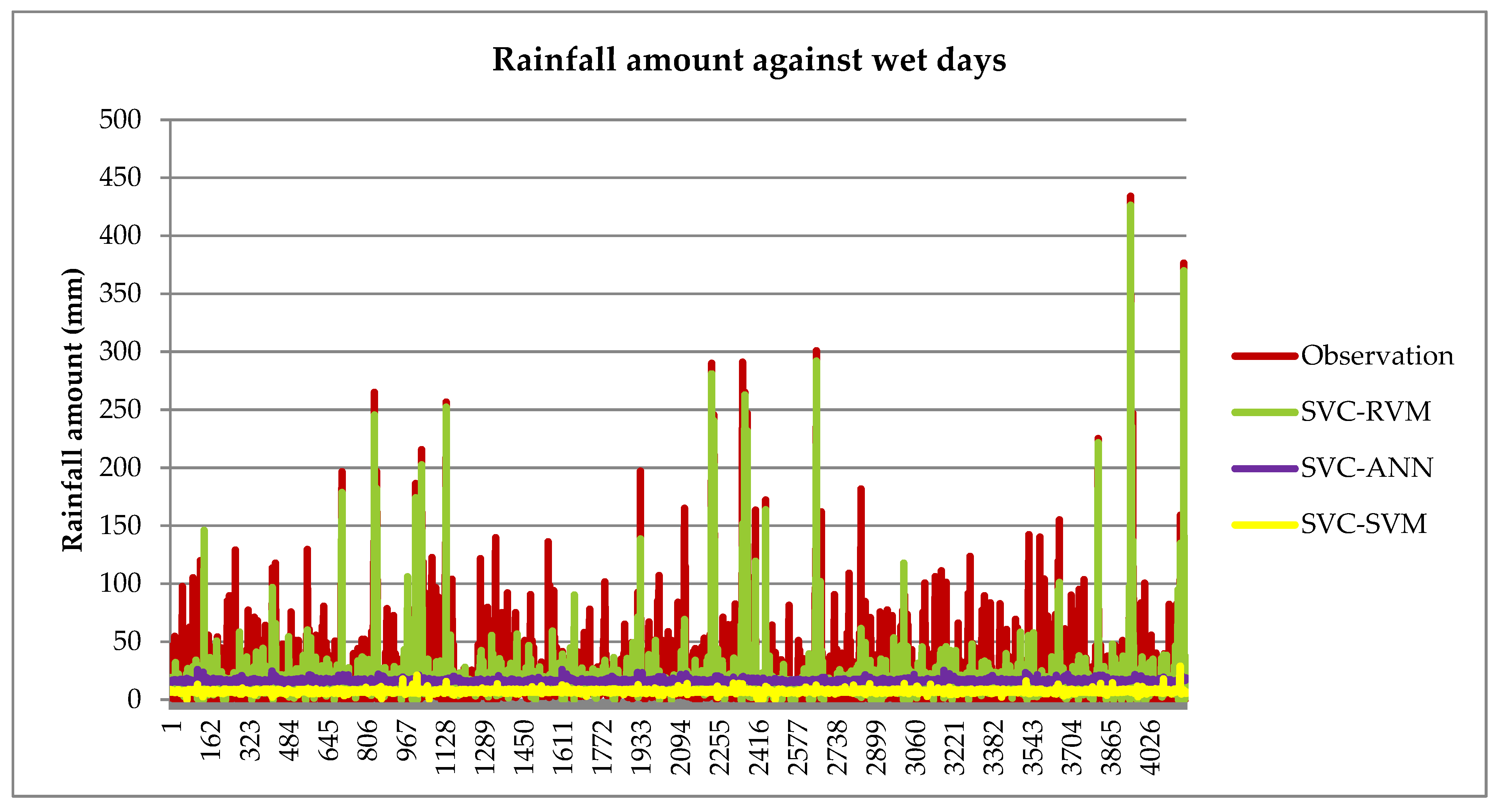
3.3.3. Results of Developing Machine Learning Techniques in Statistical Downscaling Model

Table 9. RMSE value for each hybrid model of statistical downscaling approach.

Separation Data	Calibration			Validation
	SVR-SVM	SVC-ANN	SVC-RVM	SVC-SVR	SVC-ANN	SVC-RVM
50:50	30.64	29.28	25.56	31.14	30.46	21.59
60:40	30.61	29.17	23.10	30.28	30.04	20.21
70:30	30.46	29.00	22.62	30.21	28.95	19.40
80:20	30.21	28.71	20.19	30.13	28.67	17.85

presents the performances of three hybrid models by varying ratio separation of data training to testing (80:20, 70:30, 60:40, 50:50). The best performances can be obtained from SVC-RVM with the lowest RMSE in the validation and calibration periods by 17.85 and 20.19, respectively, for the separation of 80% to 20%. In addition, the hybrid model with the worst performance is SVC-SVR, which has the highest RMSE for all separations when compared to others during the calibration and validation periods. It should be noted that for NSE values, the best model is measured when the error value approaches one [81]. From

Table 10. NSE value for each hybrid model of statistical downscaling approach.

Separation Data	Calibration			Validation
	SVC-SVR	SVC-ANN	SVC-RVM	SVC-SVR	SVC-ANN	SVC-RVM
50:50	0.01	0.11	0.31	0.06	0.16	0.53
60:40	0.09	0.12	0.35	0.16	0.22	0.60
70:30	0.12	0.29	0.46	0.26	0.33	0.69
80:20	0.16	0.23	0.61	0.30	0.34	0.81

, it is apparent that the best NSE was produced by the SVC-RVM model of 0.81 and 0.61 in the validation and calibration periods, respectively, for the separation 80% to 20%. Meanwhile, the worst NSE was indicated by the SVC-SVR model for separation 50% to 50% with 0.01 and 0.06 for the validation and calibration periods, respectively.

Based on the findings in Table 9 and Table 10, the performances of the three hybrid models were influenced by the separation of the data in identifying the best prediction model. In machine learning approaches, if the training data are limited, the parameter estimates will have a high variance. Otherwise, having less testing data leads to higher variances in measures of performance [81]. For this study, all the hybrid models represent the best performance when the separation data are 80% to 20%.

Figure 8 shows the prediction of rainfall amount using three hybrid models, namely SVC-SVR, SVC-ANN and SVC-RVM, in east-coast Peninsular Malaysia during the validation period. The Figure 8 illustrated that the statistical downscaling approach based on the SVC-RVM model performed better than other models. The model could follow the actual pattern of the daily rainfall amount in east-coast Peninsular Malaysia. Besides that, the SVC-RVM model was able to capture the general pattern of the nonlinear trend of daily rainfall amount across the long-term period. In addition, the hybrid model of SVC-RVM was useful in ensuring that similar patterns captured the features of extreme rainfall behaviour. Meanwhile, Figure 8 shows that the hybrid models of SVC-SVR and SVC-ANN performed poorly in predicting the rainfall values in a sentence period. The plot of the prediction of rainfall time series data for both hybrid models did not follow the pattern of the original rainfall data.

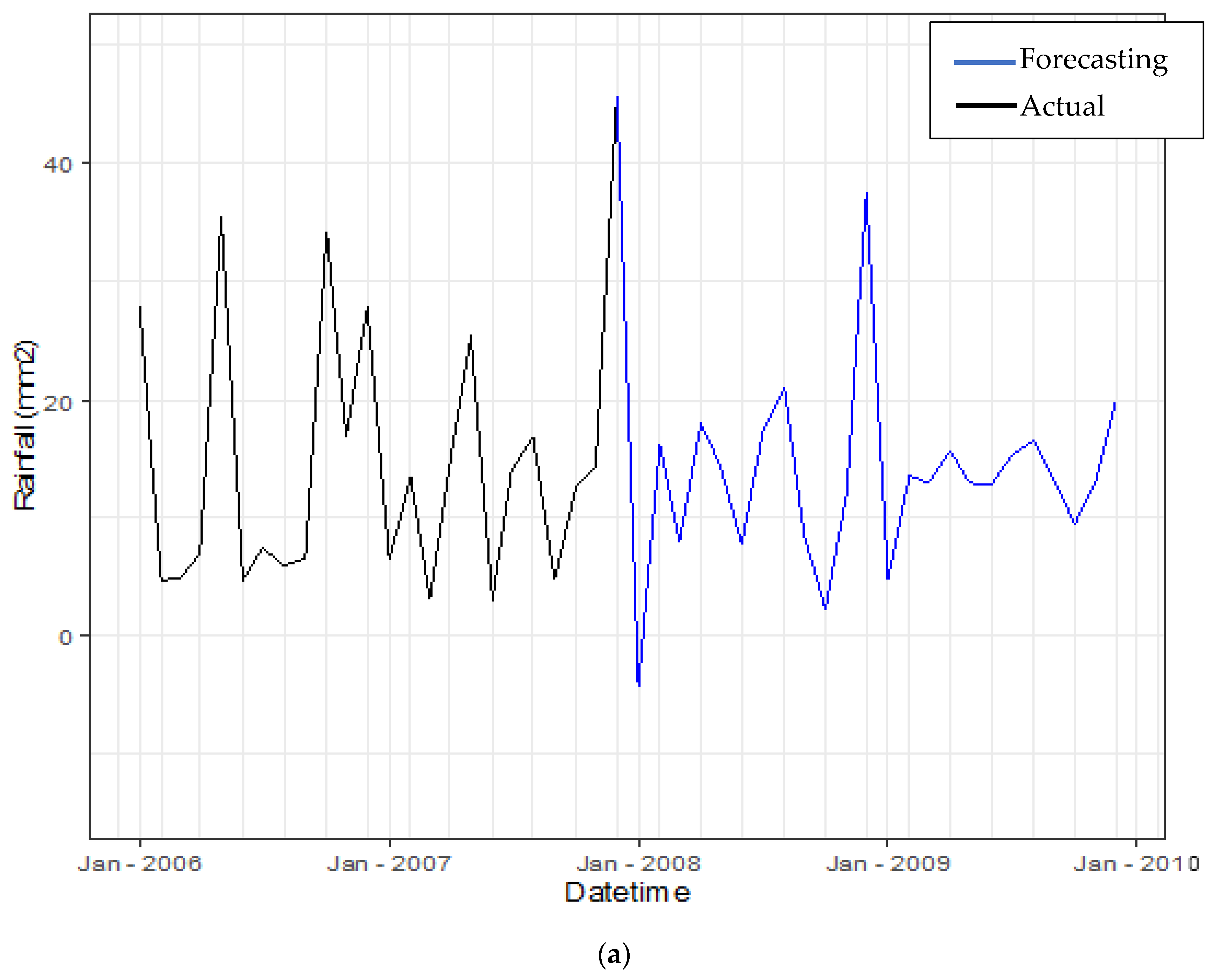
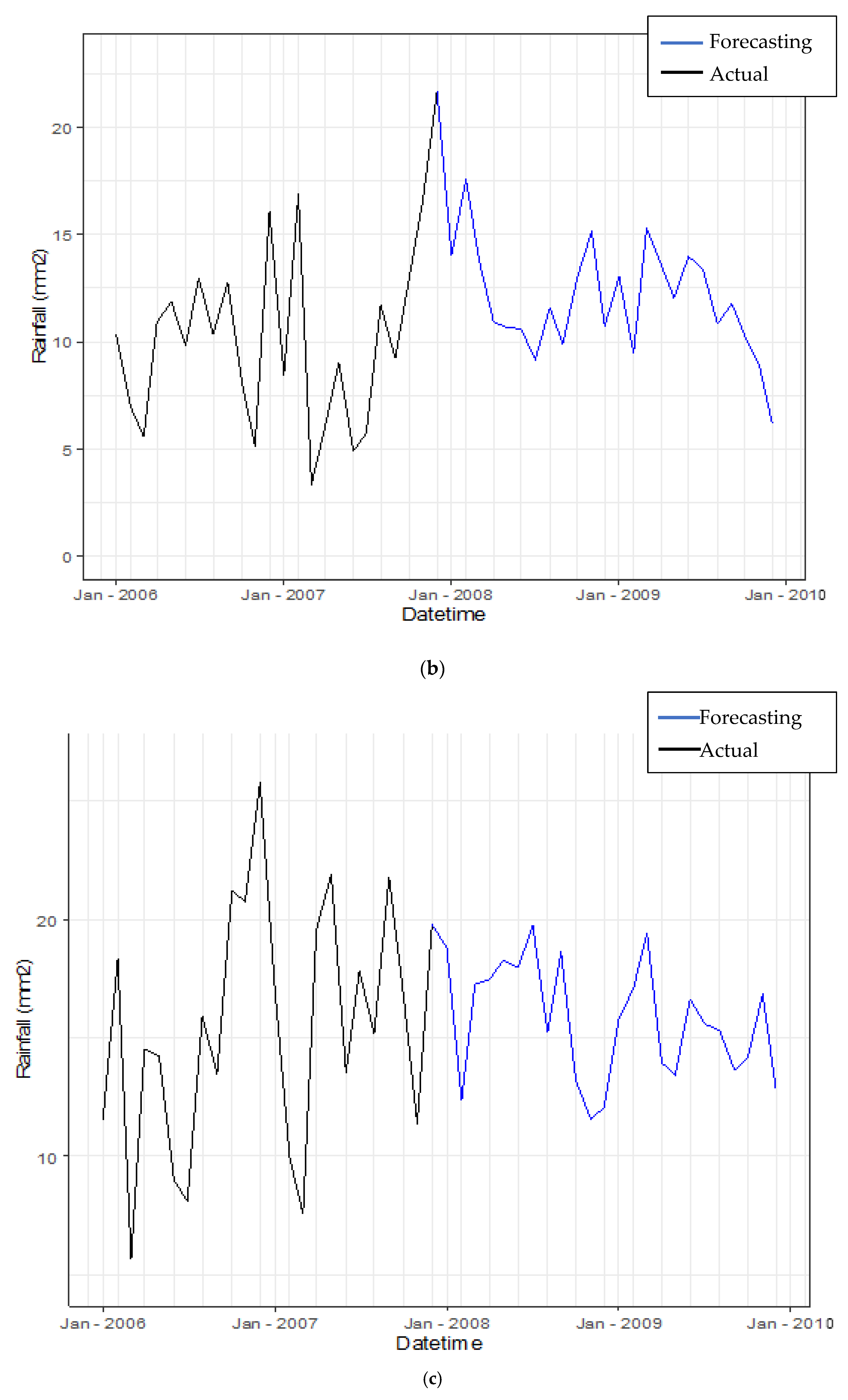
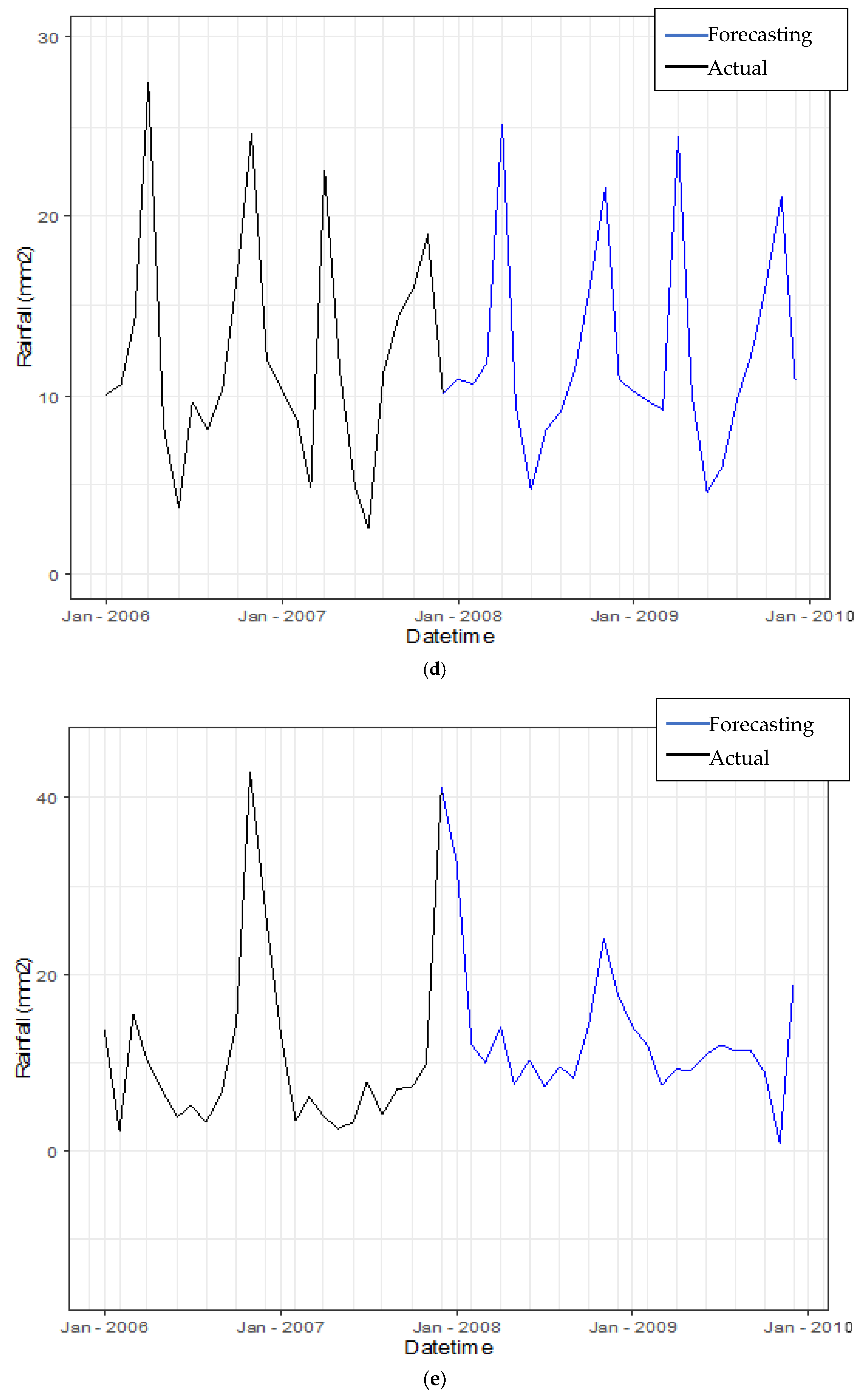
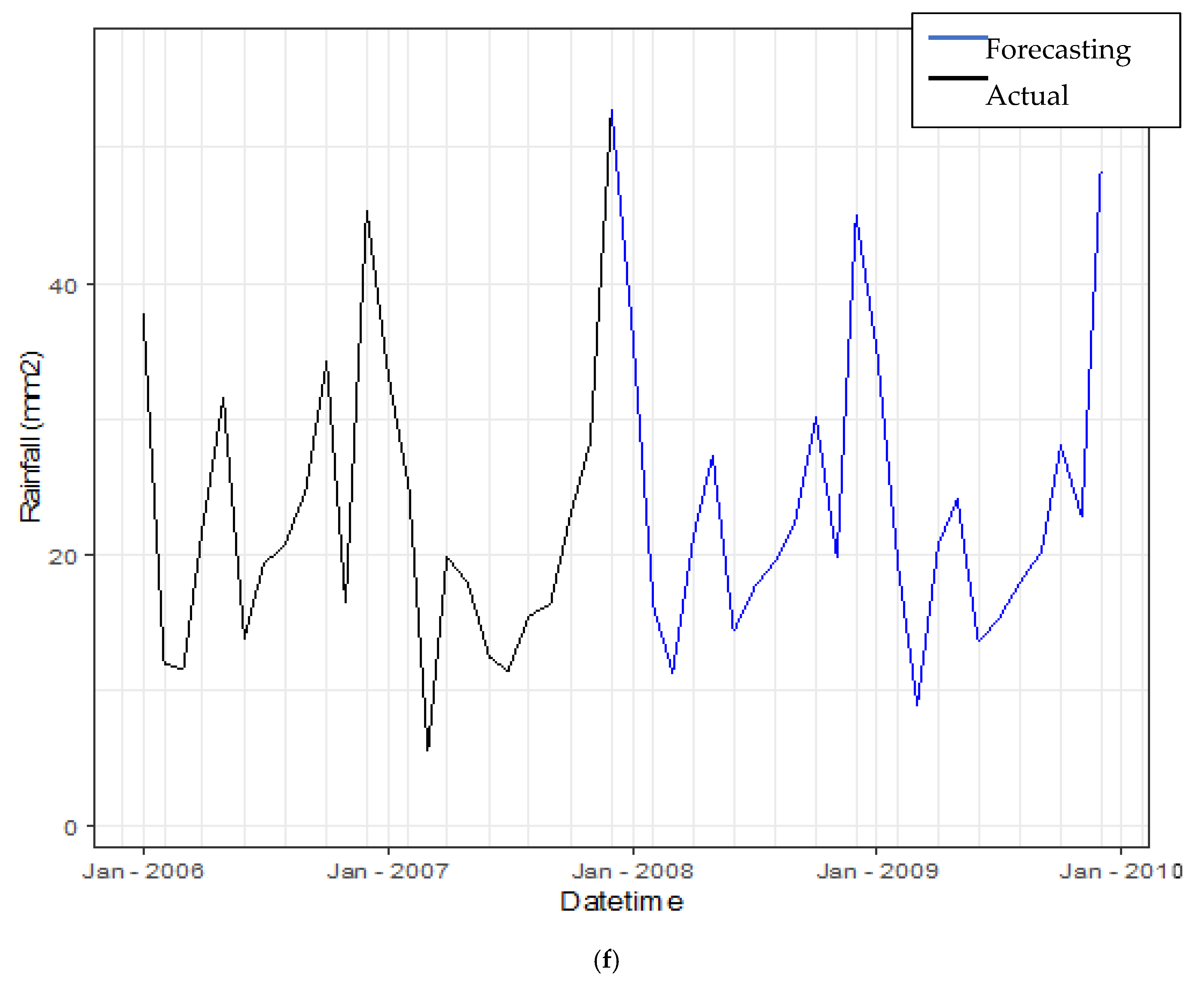
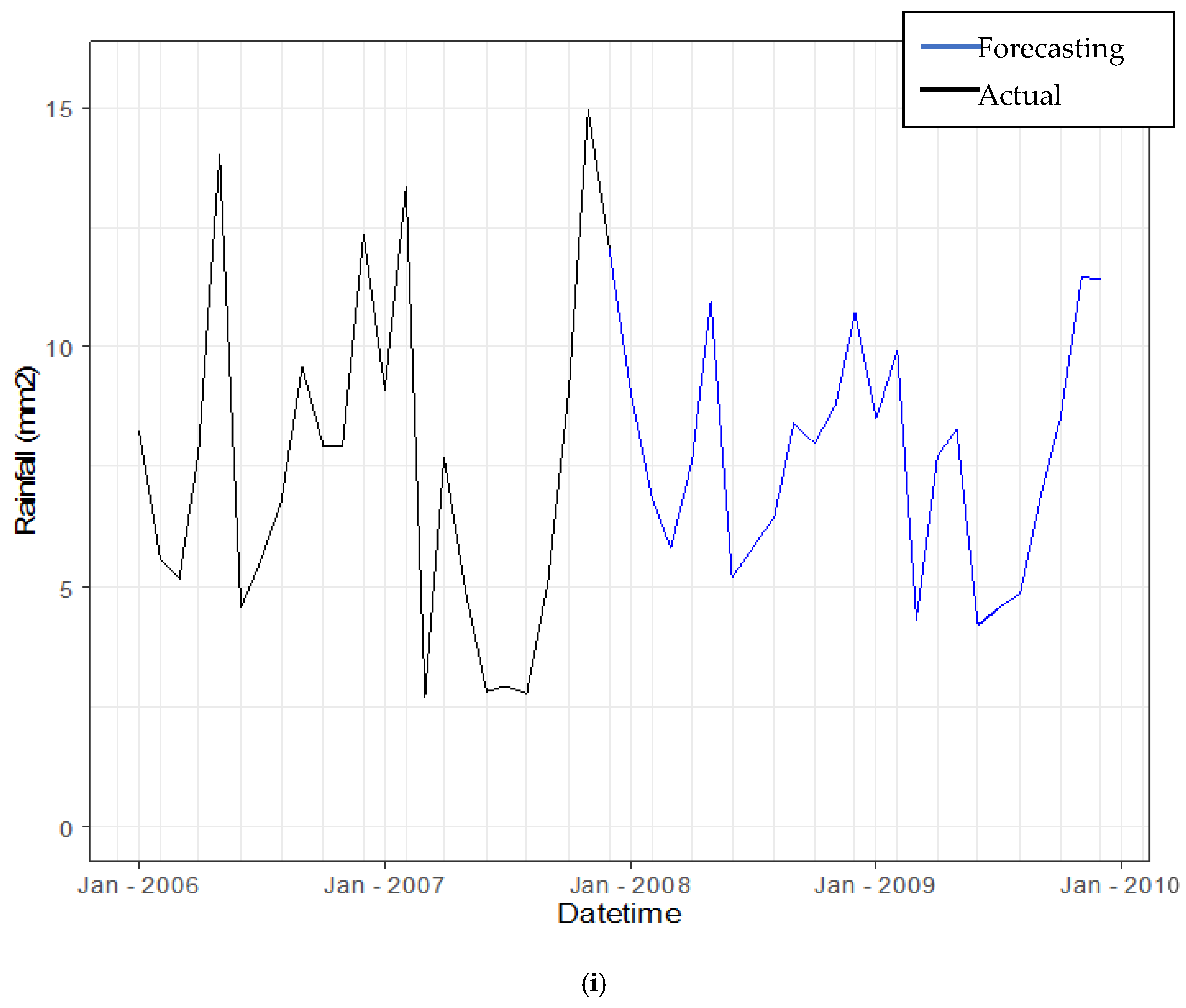
3.3.4. Forecasting Daily Rainfall by Using Hybrid Model

This section presents forecasting daily rainfall by using the hybrid model of SVC-RVM. At the time of the study, the historical data from 1 January 2006 to 31 December 2007 were used, and the future two years ahead of daily rainfall had been predicted accordingly. Figure 9a–i illustrate the available data from 1 January 2006 to 31 December 2007 and predict daily rainfall data until 31 December 2009. It is worth noting that the figures display the forecast based on each station’s daily rainfall pattern. As can be seen, the hybrid model of SVC-RVM is capable of forecasting for two years in advance based on previous patterns of daily rainfall in each station. Generally, the hybrid model’s forecasting represents the fluctuating pattern of daily rainfall for the next two years.

Table 11. Example of rainfall amount prediction from 2354 days to 2373 days.

Day	Daily (mm)	Predicted (mm)	RMSE
2354	152.00	148.74	1.81
2355	166.50	151.68	3.85
2356	17.50	18.65	1.15
2357	23.00	18.08	2.22
2358	20.00	24.67	2.16
2359	17.00	21.32	2.08
2360	60.00	55.25	2.18
2361	17.50	20.00	1.58
2362	135.00	128.04	2.64
2363	265.00	262.62	1.54
2364	5.00	9.73	2.17
2365	14.00	12.38	1.27
2366	27.50	22.56	2.22
2367	15.00	17.24	1.50
2368	9.00	5.41	2.10
2369	12.00	16.74	2.11
2370	16.80	23.26	2.54
2371	135.70	130.10	2.37
2372	13.50	11.20	1.52
2373	246.80	241.70	2.26

shows the example of rainfall amounts being predicted from the 2354th day to 2373rd day, along with the model’s RMSE value. The 2354th day until the 2373rd day were selected since the total days involved in this analysis is 4180 days, which is unsuitable for inclusion in the table. Moreover, it seems that the hybrid SVC-RVM model is an excellent model for forecasting daily rainfall amounts because of its small RMSE value. In the case of small RMSE values, the predicted and observed daily data are close to each other, indicating greater accuracy of the hybrid model.

4. Conclusions

Climate change’s impact on the hydrological cycle will result in extreme weather events such as flooding, tsunamis and others. In Malaysia, the most devastating impact of climate change experienced is flooding. Floods have a terrible impact on people because they disrupt their daily activities, and the effects can last for a week. For that reason, rainfall prediction in east-coast Peninsular Malaysia should be analysed by meteorologists to help them avoid more tragic flood incidents. In this study, the issues of rainfall prediction in east-coast Peninsular Malaysia were discovered through the process of downscaling and correlated procedures have been solved to obtain the most accurate results in rainfall data prediction.

The best hybrid model of the statistical downscaling approach in east-coast Peninsular Malaysia is the SVC-RVM model, which achieved the lowest value of RMSE while having the highest value of NSE. The prediction of rainfall values by SVC-RVM also show that this hybrid model is able to follow the actual rainfall value pattern and capture extreme rainfall values. Therefore, it can be recommended to use SVC-RVM in developing statistical downscaling for studies. In addition, the development of an SVC and SVR model in statistical downscaling approach for east-coast Peninsular Malaysia showed the best performance with the RBF kernel compared to other kernels. Moreover, for RVM-based models, the best performance is achieved by applying the Laplace kernel followed by hyperbolic tangent, polynomial, Bessel, RBF and ANOVA.

Daily rainfall was divided into two categories, dry day and wet day. Regression was then applied on the wet-day class to obtain the prediction of rainfall amount. In the future, it is possible to determine how rainy days will be classified according to more precise criteria, for example, by comparing days with light, medium and heavy rain. The methodology based on machine learning approaches demonstrates a better prediction of rainfall for this type of rainfall data. However, this study only visualizes rainfall prediction in the same year. Therefore, the proposed hybrid model in this study is recommended for future rainfall predictions spanning up to 20–30 years.

References

1. Pour, S.H.; Shahid, S.; Chung, E.-S. A Hybrid Model for Statistical Downscaling of Daily Rainfall. Procedia Eng. 2016, 154, 1424–1430. [Google Scholar] [CrossRef]
2. Schoof, J.T. Statistical Downscaling in Climatology. Geogr. Compass 2013, 7, 249–265. [Google Scholar] [CrossRef] [Green Version]
3. Lanzante, J.R.; Dixon, K.; Nath, M.J.; Whitlock, C.E.; Adams-Smith, D. Some Pitfalls in Statistical Downscaling of Future Climate. Bull. Am. Meteorol. Soc. 2018, 99, 791–803. [Google Scholar] [CrossRef]
4. Xu, R.; Chen, N.; Chen, Y.; Chen, Z. Downscaling and Projection of Multi-CMIP5 Precipitation Using Machine Learning Methods in the Upper Han River Basin. Adv. Meteorol. 2020, 2020, 8680436. [Google Scholar] [CrossRef]
5. Wilby, R.L.; Charles, S.P.; Zorita, E.; Timbal, B.; Whetton, P.; Mearns, L.O. Guidelines for Use of Climate Scenarios Developed from Statistical Downscaling Methods. Analysis 2004, 27, 1–27. [Google Scholar]
6. Chen, H.; Guo, J.; Xiong, W.; Guo, S.; Xu, C.-Y. Downscaling GCMs using the Smooth Support Vector Machine method to predict daily precipitation in the Hanjiang Basin. Adv. Atmos. Sci. 2010, 27, 274–284. [Google Scholar] [CrossRef]
7. Sachindra, D.; Ahmed, K.; Rashid, M.; Shahid, S.; Perera, B. Statistical downscaling of precipitation using machine learning techniques. Atmos. Res. 2018, 212, 240–258. [Google Scholar] [CrossRef]
8. Carleo, G.; Cirac, I.; Cranmer, K.; Daudet, L.; Schuld, M.; Tishby, N.; Vogt-Maranto, L.; Zdeborová, L. Machine learning and the physical sciences. Rev. Mod. Phys. 2019, 91, 045002. [Google Scholar] [CrossRef] [Green Version]
9. Sulaiman, N.A.; Shaharudin, S.M.; Zainuddin, N.H.; Najib, S.A.M. Improving support vector machine rainfall classification accuracy based on kernel parameters optimization for statistical downscaling approach. Int. J. Adv. Trends Comput. Sci. Eng. 2020, 9, 652–657. [Google Scholar] [CrossRef]
10. Coulibaly, P. Downscaling daily extreme temperatures with genetic programming. Geophys. Res. Lett. 2004, 31, L16203. [Google Scholar] [CrossRef]
11. Sachindra, D.A.; Huang, F.; Barton, A.; Perera, B.J.C. Least square support vector and multi-linear regression for statistically downscaling general circulation model outputs to catchment stream flows. Int. J. Clim. 2012, 33, 1087–1106. [Google Scholar] [CrossRef] [Green Version]
12. Duhan, D.; Pandey, A. Statistical downscaling of temperature using three techniques in the Tons River basin in Central India. Arch. Meteorol. Geophys. Bioclimatol. Ser. B 2014, 121, 605–622. [Google Scholar] [CrossRef]
13. Borah, D.K. Hydrologic procedures of storm event watershed models: A comprehensive review and comparison. Hydrol. Process. 2011, 25, 3472–3489. [Google Scholar] [CrossRef]
14. Shaharudin, S.M.; Ahmad, N.; Zainuddin, N.H.; Mohamed, N.S. Identification of rainfall patterns on hydrological simulation using robust principal component analysis. Indones. J. Electr. Eng. Comput. Sci. 2018, 11, 1162–1167. [Google Scholar] [CrossRef]
15. Nor, S.M.C.M.; Shaharudin, S.M.; Ismail, S.; Najib, S.A.M.; Tan, M.L.; Ahmad, N. Statistical Modeling of RPCA-FCM in Spatiotemporal Rainfall Patterns Recognition. Atmosphere 2022, 13, 145. [Google Scholar] [CrossRef]
16. Shaharudin, S.M.; Nor, S.M.C.M.; Tan, M.L.; Samsudin, M.S.; Azid, A.; Ismail, S. Spatial Torrential Rainfall Modelling in Pattern Analysis Based on Robust PCA Approach. Pol. J. Environ. Stud. 2021, 30, 3221–3230. [Google Scholar] [CrossRef]
17. Nayak, P.C.; Sudheer, K.P.; Rangan, D.M.; Ramasastri, K.S. Short-term flood forecasting with a neurofuzzy model. Water Resour. Res. 2005, 41, W04004. [Google Scholar] [CrossRef] [Green Version]
18. Costabile, P.; Macchione, F. Enhancing river model set-up for 2-D dynamic flood modelling. Environ. Model. Softw. 2015, 67, 89–107. [Google Scholar] [CrossRef]
19. Van den Honert, R.C.; McAneney, J. The 2011 Brisbane Floods: Causes, Impacts and Implications. Water 2011, 3, 1149–1173. [Google Scholar] [CrossRef] [Green Version]
20. Lee, T.H.; Georgakakos, K.P. Operational Rainfall Prediction on Meso-γ Scales for Hydrologic Applications. Water Resour. Res. 1996, 32, 987–1003. [Google Scholar] [CrossRef]
21. Shrestha, D.L.; Robertson, D.E.; Wang, Q.J.; Pagano, T.C.; Hapuarachchi, P. Evaluation of numerical weather prediction model precipitation forecasts for use in short-term streamflow forecasting. Hydrol. Earth Syst. Sci. Discuss. 2012, 9, 12563–12611. [Google Scholar]
22. Chen, S.-T.; Yu, P.-S.; Tang, Y.-H. Statistical downscaling of daily precipitation using support vector machines and multivariate analysis. J. Hydrol. 2010, 385, 13–22. [Google Scholar] [CrossRef]
23. Aftab, S.; Ahmad, M.; Hameed, N.; Salman, M.; Ali, I.; Nawaz, Z. Rainfall Prediction using Data Mining Techniques: A Systematic Literature Review. Int. J. Adv. Comput. Sci. Appl. 2018, 9, 090518. [Google Scholar] [CrossRef] [Green Version]
24. Loyola R, D.G.; Pedergnana, M.; García, S.G. Smart sampling and incremental function learning for very large high dimensional data. Neural Netw. 2016, 78, 75–87. [Google Scholar] [CrossRef] [Green Version]
25. Katal, A.; Wazid, M.; Goundar, R. Big Data: Issues, Challenges, Tools and Good Practices. Proceeding of the 2013 Sixth International Conference on Contemporary Computing, Noida, India, 8–10 August 2013. [Google Scholar]
26. Tanwar, S.; Ramani, T.; Tyagi, S. Dimensionality reduction using PCA and SVD in big data: A comparative case study. In Future Internet Technologies and Trends; Patel, Z., Gupta, S., Eds.; Springer: Cham, Switzerland, 2018; Volume 220, pp. 116–125. [Google Scholar]
27. Saini, O.; Sharma, P.S. A Review on Dimension Reduction Techniques in Data Mining. Comput. Eng. Intell. Syst. 2018, 9, 7–14. [Google Scholar]
28. Brence, J.R.; Brown, D.E. Improving the Robust Random Forest Regression Algorithm. Systems and Information Engineering Technical Papers. 2006, pp. 1–18. Available online: http://citeseerx.ist.psu.edu/viewdoc/download?doi=10.1.1.712.588&rep=rep1&type=pdf (accessed on 11 March 2022).
29. Ho, T.K. Random Decision Forests Tin Kam Ho Perceptron training. In Proceedings of the 3rd International Conference on Document Analysis and Recognition, Montreal, QC, Canada, 14–16 August 1995. [Google Scholar]
30. Breiman, L. Random Forests. Mach. Lang. 2001, 45, 5–32. [Google Scholar]
31. Jollife, I.T.; Cadima, J. Principal component analysis: A review and recent developments. Philos. Trans. R. Soc. A Math. Phys. Eng. Sci. 2016, 374, 20150202. [Google Scholar] [CrossRef]
32. Yamini, O.; Ramakrishna, S. A Study on Advantages of Data Mining Classification Techniques. Int. J. Eng. Res. 2015, V4, 090815. [Google Scholar] [CrossRef]
33. Tripathi, S.; Srinivas, V.; Nanjundiah, R.S. Downscaling of precipitation for climate change scenarios: A support vector machine approach. J. Hydrol. 2006, 330, 621–640. [Google Scholar] [CrossRef]
34. Advantages of Support Vector Machines (SVM). Available online: https://iq.opengenus.org/advantages-of-svm/ (accessed on 11 March 2022).
35. Raghavendra, S.; Deka, P.C. Support vector machine applications in the field of hydrology: A review. Appl. Soft Comput. J. 2014, 19, 372–386. [Google Scholar] [CrossRef]
36. Lin, S.; Zhang, S.; Qiao, J.; Liu, H.; Yu, G. A parameter choosing method of SVR for time series prediction. In Proceedings of the 2008 9th International Conference for Young Computer Scientists, Zhangjiajie, China, 18–21 November 2008. [Google Scholar]
37. E Wang, J.; Qiao, J.Z. Parameter Selection of SVR Based on Improved K-Fold Cross Validation. Appl. Mech. Mater. 2013, 462–463, 182–186. [Google Scholar] [CrossRef]
38. Mishra, N.; Soni, H.K.; Sharma, S.; Upadhyay, A.K. Development and Analysis of Artificial Neural Network Models for Rainfall Prediction by Using Time-Series Data. Int. J. Intell. Syst. Appl. 2018, 10, 16–23. [Google Scholar] [CrossRef]
39. Kumar, P.; Praveen, T.V.; Prasad, M.A. Artificial Neural Network Model for Rainfall-Runoff—A Case Study. Int. J. Hybrid. Inf. Technol. 2016, 9, 263–272. [Google Scholar] [CrossRef]
40. Tipping, M.E. Sparse Bayesian Learning and the Relevance Vector Machine. J. Mach. Learn. Res. 2001, 1, 211–244. [Google Scholar]
41. Ghosh, S.; Mujumdar, P. Statistical downscaling of GCM simulations to streamflow using relevance vector machine. Adv. Water Resour. 2008, 31, 132–146. [Google Scholar] [CrossRef]
42. Samui, P.; Dixon, B. Application of support vector machine and relevance vector machine to determine evaporative losses in reservoirs. Hydrol. Process. 2011, 26, 1361–1369. [Google Scholar] [CrossRef]
43. Hong, S.; Lynn, H.S. Accuracy of random-forest-based imputation of missing data in the presence of non-normality, non-linearity, and interaction. BMC Med. Res. Methodol. 2020, 20, 199. [Google Scholar] [CrossRef]
44. Liaw, A.; Wiener, M. Classification and Regression by random Forest. R News 2002, 2, 18–22. [Google Scholar]
45. Stekhoven, D.J.; Bühlmann, P. Missforest-Non-parametric missing value imputation for mixed-type data. Bioinformatics 2012, 28, 112–118. [Google Scholar] [CrossRef] [Green Version]
46. Ayesha, S.; Hanif, M.K.; Talib, R. Overview and comparative study of dimensionality reduction techniques for high dimensional data. Inf. Fusion 2020, 59, 44–58. [Google Scholar] [CrossRef]
47. Bethere, L.; Sennikovs, J.; Bethers, U. Climate indices for the Baltic states from principal component analysis. Earth Syst. Dyn. 2017, 8, 951–962. [Google Scholar] [CrossRef] [Green Version]
48. Denguir, M.; Sattler, S.M. A dimensionality-reduction method for test data. Proceeding of the 2017 IEEE 22nd International Mixed-Signals Test Workshop (IMSTW 2017), Thessaloniki, Greece, 3–5 July 2017. [Google Scholar]
49. Ghosh, S. SVM-PGSL coupled approach for statistical downscaling to predict rainfall from GCM output. J. Geophys. Res. Earth Surf. 2010, 115, 1–19. [Google Scholar] [CrossRef] [Green Version]
50. Huang, C.-L.; Wang, C.-J. A GA-based feature selection and parameters optimization for support vector machines. Expert Syst. Appl. 2006, 31, 231–240. [Google Scholar] [CrossRef]
51. Campozano, L.; Tenelanda, D.; Sanchez, E.; Samaniego, E.; Feyen, J. Comparison of Statistical Downscaling Methods for Monthly Total Precipitation: Case Study for the Paute River Basin in Southern Ecuador. Adv. Meteorol. 2016, 2016, 6526341. [Google Scholar] [CrossRef]
52. Halik, G.; Anwar, N.; Santosa, B.; Edijatno. Reservoir Inflow Prediction under GCM Scenario Downscaled by Wavelet Transform and Support Vector Machine Hybrid Models. Adv. Civ. Eng. 2015, 2015, 515376. [Google Scholar] [CrossRef] [Green Version]
53. Lu, L. Optimal Gamma and C for Epsilon Support Vector Regression with RBF Kernels. Available online: http://arxiv.org/abs/1506.03942 (accessed on 19 August 2021).
54. Berrar, D. Cross-validation. Encycl. Bioinform. Comput. Biol. ABC Bioinform. 2018, 1–3, 542–545. [Google Scholar]
55. Borra, S.; Di Ciaccio, A. Measuring the prediction error. A comparison of cross-validation, bootstrap and covariance penalty methods. Comput. Stat. Data Anal. 2010, 54, 2976–2989. [Google Scholar] [CrossRef]
56. Okkan, U.; Serbes, Z.A.; Samui, P. Relevance vector machines approach for long-term flow prediction. Neural Comput. Appl. 2014, 25, 1393–1405. [Google Scholar] [CrossRef]
57. Erdal, H.I.; Karakurt, O. Advancing monthly streamflow prediction accuracy of CART models using ensemble learning paradigms. J. Hydrol. 2013, 477, 119–128. [Google Scholar] [CrossRef]
58. Fatihah, C.O.S.; Hila, Z.N.; Shaharudin, S.M.; Safiih, L.M.; Nikenasih, B.; Farizie, A.M.K. Bootstrapping the Multilayer Feedforward Propagation System for Predicting the Arrival Guest in Malaysia. Rev. Int. Geogr. Educ. 2021, 11, 754–763. [Google Scholar]
59. Govindaraju, R.S. Artificial Neural Networks in Hydrology. II: Hydrologic Applications. J. Hydrol. Eng. 2000, 5, 124–137. [Google Scholar]
60. Mekanik, F.; Imteaz, M.; Gato-Trinidad, S.; Elmahdi, A. Multiple regression and Artificial Neural Network for long-term rainfall forecasting using large scale climate modes. J. Hydrol. 2013, 503, 11–21. [Google Scholar] [CrossRef]
61. Top 4 Advantages and Disadvantages of Support Vector Machine or SVM. Available online: https://dhirajkumarblog.medium.com/top-4-advantages-and-disadvantages-of-support-vector-machine-or-svm-a3c06a2b107 (accessed on 20 November 2021).
62. Xia, Y. Correlation and association analyses in microbiome study integrating multiomics in health and disease. Prog. Mol. Biol. Transl. Sci. 2020, 171, 309–491. [Google Scholar] [CrossRef] [PubMed]
63. Pal, M. Kernel methods in remote sensing: A review. ISH J. Hydraul. Eng. 2009, 15, 194–215. [Google Scholar] [CrossRef]
64. Cummins, N.; Sethu, V.; Epps, J.; Krajewski, J. Relevance vector machine for depression prediction. Interspeech 2015, 2015, 110–114. [Google Scholar] [CrossRef]
65. Presti, R.L.; Barca, E.; Passarella, G. A methodology for treating missing data applied to daily rainfall data in the Candelaro River Basin (Italy). Environ. Monit. Assess. 2008, 160, 1. [Google Scholar] [CrossRef] [PubMed]
66. Moritz, S.; Sardá, A.; Bartz-Beielstein, T.; Zaefferer, M.; Stork, J. Comparison of different Methods for Univariate Time Series Imputation in R. arXiv 2015, arXiv:1510.03924a. [Google Scholar]
67. Zhang, Y.; Wu, L. Classification of Fruits Using Computer Vision and a Multiclass Support Vector Machine. Sensors 2012, 12, 12489–12505. [Google Scholar] [CrossRef]
68. Azid, A.; Juahir, H.; Toriman, M.E.; Kamarudin, M.K.A.; Saudi, A.S.M.; Hasnam, C.N.C.; Aziz, N.A.A.; Azaman, F.; Latif, M.T.; Zainuddin, S.F.M.; et al. Prediction of the Level of Air Pollution Using Principal Component Analysis and Artificial Neural Network Techniques: A Case Study in Malaysia. Water Air Soil Pollut. 2014, 225, 2063. [Google Scholar] [CrossRef]
69. Dominick, D.; Juahir, H.; Latif, M.T.; Zain, S.M.; Aris, A.Z. Spatial assessment of air quality patterns in Malaysia using multivariate analysis. Atmos. Environ. 2012, 60, 172–181. [Google Scholar] [CrossRef]
70. Liu, C.-W.; Lin, K.-H.; Kuo, Y.-M. Application of factor analysis in the assessment of groundwater quality in a blackfoot disease area in Taiwan. Sci. Total Environ. 2003, 313, 77–89. [Google Scholar] [CrossRef]
71. Nanda, M.A.; Seminar, K.B.; Nandika, D.; Maddu, A. A Comparison Study of Kernel Functions in the Support Vector Machine and Its Application for Termite Detection. Information 2018, 9, 5. [Google Scholar] [CrossRef] [Green Version]
72. Understanding Support Vector Machine (SVM) Algorithm from Examples (Along with Code). Available online: https://www.analyticsvidhya.com/blog/2017/09/understaing-support-vector-machine-example-code/ (accessed on 21 August 2021).
73. Berzofsky, M.; Biemer, P.; Kalsbeek, W. A Brief History of Classification Error Models. In Proceedings of the Joint Statistical Meetings, Denver, CO, USA, 3–7 August 2008. [Google Scholar]
74. Regression Techniques You Should Know! Available online: https://www.analyticsvidhya.com/blog/2015/08/comprehensive-guide-regression/ (accessed on 27 July 2020).
75. Vapnik, V.N. The Nature of Statistical Learning Theory, 1st ed.; Springer: New York, NY, USA, 1995; pp. 110–123. [Google Scholar]
76. Ali, A.H.; Abdullah, M.Z. An efficient model for data classification based on SVM grid parameter optimization and PSO feature weight selection. Int. J. Integr. Eng. 2020, 12, 1–12. [Google Scholar]
77. Pattern Recognition Tools 37 Steps. Available online: http://37steps.com/4859/cross-validation/ (accessed on 31 September 2020).
78. Tipping, M.E. The relevance vector machine. Adv. Neural Inf. Process. Syst. 2000, 12, 653–658. [Google Scholar]
79. Assessing the Fit of Regression Models. Available online: https://www.theanalysisfactor.com/assessing-the-fit-of-regression-models/ (accessed on 11 July 2020).
80. Bhattacharya, D.; Nisha, M.G.; Pillai, G. Relevance vector-machine-based solar cell model. Int. J. Sustain. Energy 2014, 34, 685–692. [Google Scholar] [CrossRef]
81. Knoben, W.J.M.; Freer, J.E.; Woods, R.A. Technical note: Inherent benchmark or not? Comparing Nash–Sutcliffe and Kling–Gupta efficiency scores. Hydrol. Earth Syst. Sci. 2019, 23, 4323–4331. [Google Scholar] [CrossRef] [Green Version]
Figure 1. The location of rainfall and atmospheric stations in east-coast Peninsular Malaysia.
Symmetry 14 00927 g001
Figure 2. Flowchart of statistical downscaling method.
Symmetry 14 00927 g002
Figure 3. The steps in selecting the predictor by using Principal Component Analysis (PCA).
Symmetry 14 00927 g003
Figure 4. Architecture of the Neural Network Model used in this study.
Symmetry 14 00927 g004
Figure 5. Flowchart of developed statistical downscaling model of SVC-RVM.
Symmetry 14 00927 g005
Figure 6. Correlation visualization of missing and non-missing data for predictor variables.
Symmetry 14 00927 g006
Figure 7. Turning parameter ε by 10th-fold cross validation.
Symmetry 14 00927 g007
Figure 8. Performance of three hybrid models in predicting daily rainfall amount in validation period.
Symmetry 14 00927 g008
Figure 9. Forecasting daily rainfall for stations of (a) Kota Bharu, (b) Sek. Keb. Kg. Jabi, (c) Kg. Merang, (d) Gua Musang, (e) Stor JPS Kuala Terengganu, (f) Kg Menerong, (g) Sek. Men. Sultan Omar, (h) Sek. Keb. Kemasek and (i) JPS Kemaman.
Symmetry 14 00927 g009aSymmetry 14 00927 g009bSymmetry 14 00927 g009cSymmetry 14 00927 g009dSymmetry 14 00927 g009eSymmetry 14 00927 g009f