Abstract
An echelon-use lithium-ion battery (EULB) refers to a powered lithium-ion battery used in electric vehicles when the battery capacity is attenuated to less than 80% and greater than 20%. Aiming at the degradation of the performance of the EULB and the unclear initial value of the state of energy (SOE), estimations of the state of power (SOP) of an EULB are not accurate. An SOP estimation method based on an adaptive dual unscented Kalman filter (ADUKF) is proposed. First, the second-order resistor-capacitance symmetry equivalent model (SRCSEM) of the EULB is established. Second, an unscented transformation (UT) is introduced and the battery parameters estimated by the ADUKF: (a) the SOE is estimated based on an adaptive unscented Kalman filtering (AUKF) algorithm, that uses the observation noise equation γk, Rk and the processes noise equation qk, Qk, and (b) the ohmic internal resistance (OIR) and actual capacity (AC) are estimated based on the aforementioned algorithm, which uses the observation noise equation γθ,k, Rθ,k and the process noise equation qθ,k, Qθ,k. Third, the working voltage and OIR are predicted using optimal estimation, and the SOP of the EULB is estimated. MATLAB simulation results show that EULB symmetry capacity decays to 80%, 60%, 40%, and 20% of rated capacity, the proposed algorithm is adaptive regardless of whether the initial SOE value is consistent with the actual value, and the estimation error of the EULB’s SOP is less than 3.28%, showing high accuracy. The results of this study can provide valuable reference for estimating EULB parameters, and help to understand the usage behavior of retired batteries.
1. Introduction
With an increase in the number of retired lithium-ion batteries, the EULB has attract-ed much attention. An EULB refers to a lithium iron phosphate powered lithium battery used in electric vehicles (EVs) when the capacity is attenuated to greater than 20% and less than 80%, which is used for power backup and energy storage of communication base stations.
In order to achieve effective utilization of lithium-ion batteries throughout their life cycle, many researches are devoted to the echelon-use of retired EVs batteries in the references. Neubauer et al. [1] started the study of battery secondary utilization in 2010. In references [2,3], Tong and Omar verified the feasibility of re-application of echelon-use batteries in photovoltaic charging stations, and completed more than 1000 charge discharge cycles at 1 C and 80% discharge depth. Jiang et al. [4], who estimated the residual capacity of echelon-use batteries by the regression method verified the feasibility of the method with an estimated error within 3%. In reference [5], Schuster et al. studied the influence of battery capacity and impedance parameter aging on state of health (SOH) estimation. Zhang et al. [6] conducted performance tests on retired EV battery modules, coordinating the test accuracy and test time. Therefore, the retired batteries were shown to still have a high ability in discharge, indicating that an EULB energy storage system can be applied to achieve the power requirement of an electrical grid.
Although the retired battery still has a high discharge capacity, it is difficult to ensure the safety of EULB due to performance degradation and capacity attenuation. As a result, large-scale promotion and utilization of echelon-use batteries are difficult. As an important parameter of battery safety control and energy recovery, SOP (state of power) has attracted more and more attention. Common methods to estimate SOP include battery experiment and model method. In references [7,8], the United States Advanced Battery Consortium (USABC) adopted a battery experimental method that has the advantage of strong practicability. In references [9,10], the battery experimental method is a test method adopted by Fang and Yu. Owing to disadvantages of testing being complicated and equipment being required, the use of the estimation method has increased based on the equivalent circuit model. The equivalent circuit model was used to estimate SOP firstly in reference [11]. In references [12,13,14,15], the first-order equivalent circuit model was used to estimate SOP. In reference [15], the first-order model was adopted to estimate state of charge (SOC), SOH, and SOP based on an unscented Kalman filter, but observation and process errors were not considered. The second-order resistor-capacitance equivalent model (SRCSEM) was used to estimate SOP in [16,17,18,19,20,21,22,23,24]. In [23], the adaptive estimation algorithm was adopted, and the estimation accuracy of SOP was 4.8%, which was not high. Reference [24] estimated SOC, SOE (state of energy), SOP, and SOH based on SRCSEM, which achieved high accuracy, but lacked adaptive research. The third-order equivalent model was adopted in [25] to carry out SOP estimation. Owing to the high order of the equivalent model, a large amount of calculation is required. Lin [16,26] proposed a new polarization voltage (NPV) model based on current and time, and the overall error of estimated accuracy of SOP was found to be approximately 5%. Liu [27] estimated SOP based on a fractional model, with a maximum error of 1.34% and high accuracy, but an insufficient adaptive ability.
The traditional SOP estimation method either has poor estimation accuracy or inadequate adaptive ability, and neither of them can be satisfied at the same time. Aiming at the degradation of EULB performance, therefore, an important research direction of battery SOP estimation is to improve the accuracy and adaptive ability of the algorithm.
SOE is an important parameter of the battery management system, which is the ratio of the remaining available energy to the maximum available energy. The performance degradation of EULB reduces the maximum available energy, thus reducing the accuracy of SOE estimation. However, few people have studied this topic in SOE estimation methods at present.
Owing to the above problems of EULB performance, in the present work an adaptive dual unscented Kalman filter (ADUKF) algorithm is first applied based on the SRCSEM. That is, based on the ADUKF algorithm used to estimate the SOE, ohmic internal resistance (OIR), and actual capacity (AC), the optimal estimation is used to predict the working voltage and OIR is used to estimate the EULB’s SOP. Finally, the estimation method of the EULB’s SOP is established. It can not only improve the estimation accuracy of SOP, but also enhance the self-adaptability of SOP estimation. It provides safety guarantees for the promotion and utilization of the EULB.
The objective of this paper is to propose an effective SOP estimation method for EULB and analyze the influence of the degradation of the performance of EULB. There are four original contributions as follows:
- (1)
- Owing to the degradation of EULB, the SOE initial value is not clear, thus parameter estimation of EULB is discussed.
- (2)
- Aiming at unclear SOE of EULB, UT is adopted and an adaptive method used, that can be adjusted adaptively to estimate the accuracy based on the observation noise equation γk, Rk and the processes noise equation qk, Qk.
- (3)
- To improve the accuracy of SOP estimation, UT and ADUKF are adopted to estimate the parameters of EULB based on the observation noise equation γθ,k, Rθ,k and the process noise equation qθ,k, Qθ,k aimed at performance attenuation of the EULB and the inaccuracy of AC and OIR.
- (4)
- It provides a theoretical basis for the effective utilization of the whole life cycle of a lithium-ion battery.
2. SRCSEM of EULB
Owing to the complex nonlinear system of the lithium-ion battery, in order to simulate the characteristics of the battery more accurately, it is necessary to select a higher-order battery equivalent model. The SRCSEM can not only better reflect the static and dynamic characteristics of EULB, but also can reduce the order of the model, which can reduce the calculation and makes it easy to apply to engineering [28,29,30].
As shown in Figure 1, the second-order resistor-capacitance symmetry model is used as the equivalent model of an EULB. is the long time constant, which is used to simulate the process of rapid change of discharge voltage in the dynamic characteristics of EULB; is the short time constant, which is used to simulate the process of slow and stable discharge voltage in the dynamic characteristics of EULB. In addition, is the open circuit voltage (OCV) of EULB, is the working voltage of EULB, is the charge/discharge current of EULB, and is the OIR of the EULB.
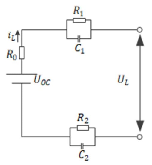
Figure 1.
The SRCSEM.
According to Figure 1, the discrete state equation of the second-order resistor-capacitance symmetry equivalent circuit of the EULB is as follows:
According to Figure 1, the discrete observation equation of the second-order resistor-capacitance equivalent circuit of the EULB is as follows:
As
Thus
where, are the SOE of the EULB at k, k + 1 time in discrete state; is the energy of the EULB; is the charge/discharge current at k time in discrete state; is the working voltage of the EULB at k time in discrete state; is the sampling period; are the estimated voltage values of at k, k + 1 time in discrete state; are the estimated voltage values of at k, k + 1 time in discrete state; are independent system noises, is a 3-dimensional vector quantity; and is the OCV of the EULB corresponding to the SOE value of the EULB at the k time in discrete state.
3. Model Parameter Identification
3.1. OCV
The OCV :
- (1)
- Charging current is 36 A and cut-off voltage is 3.65 V.
- (2)
- Discharging current is 36 A and cut-off voltage is 2.5 V. Record the discharge voltage .
- (3)
- Charging current is 36 A and cut-off voltage is 3.65 V. Record the charge voltage .
- (4)
- The OCV U_OC is as follows:
3.2. OIR
Based on Ohm’s law, the OIR is as follows:
where is the charge/discharge current of EULB and is voltage change [31,32].
3.3. Polarization Resistance
The working voltage , charge/discharge current and OCV of the EULB is collected through the charge/discharge test. Model parameter identification based on the least square method is not repeated in this paper because the method is described in detail in references [28,32].
4. SOP Estimation
In this paper, an ADUKF algorithm is applied based on the SRCSEM: the first is to estimate the SOE based on the AUKF algorithm; the second is to estimate the OIR and AC based on the AUKF algorithm [33,34].
4.1. UT
UT is the core technology of unscented Kalman filter (UKF). The idea of UT is to approximate the distribution of a probability density function through a set of carefully selected sample points and the corresponding weights of sample points. A certain number of sigma points are selected from the prior distribution according to a certain strategy, and nonlinear transformation is performed on each sigma point to obtain the corresponding transformed sampling points. In addition, the posterior mean and variance are calculated by weighting these sample points. The sample points obtained by UT are not linearized, nor are higher-order terms lost, thus the accuracy of UT is higher than that of the extended Kalman filter algorithm.
For any nonlinear function , around the n-dimensional state variable with mean value of and variance of , 2n + 1 sigma points and corresponding weights can be selected through the following UT process.
In the above formula, is the column or row of the square root of . is the scale factor used to represent the range of sampling points around equilibrium value points, and is the weight of corresponding sample points. In this paper, .
From , the sample point with nonlinear transformation can be obtained:
Then, statistical characteristics of output sampling points can be obtained by weighted approximation:
4.2. SOE Estimation Based on ADUKF
According to Equations (3) and (4), the variable of the echelon-use battery system is the SOE. In this paper, the ohmic resistance and actual capacity of the echelon-use battery are added into the state variable due to the serious problems of the increase of ohmic resistance and the decline of the actual capacity of the echelon-use battery. The system state variable has three parameters: SOE, ohm internal resistance, and the actual capacity [35,36].
The state and observation equations are as follows:
where, is the state variable ohmic internal resistance and actual capacity,, to reduce the amount of calculation, whenever , that is, the reduction per exceeds 0.72 Ah, the values of in Equations (1) and (2) are updated, ; is the system state variable; is the input of the system and is the echelon-use battery current; and is the system observation variable and is the working voltage of the echelon-use battery.
In this paper, the error covariance matrices of the zero-mean Gaussian white noise are .
The algorithm flow is as follows:
- Step 1: Inialize is as follows:
- Step 2: Generating sigma points:
- Step 3: Time update of the system state is as follows
- Step 4: Status update of the system state is as follows:The Kalman gain is as follows:The optimal estimation of state variables is as follows:The optimal estimate of the covariance is as follows:
- Step 5: Process noise mean and covariance equation is as follows:
- Step 6: Observe the noise mean and covariance equation as follows:where , b is the forgetting factor of x, 0 < b < 1, ; and are the estimation and optimal estimation of the state variable at k time, respectively; and are the estimated value and actual observation value at k time; and and are, respectively, the estimation and optimal estimation of the error covariance at k time.
4.3. OIR and AC Estimation Based on AUKF
The state and observation formulas of the system with the newly added state parameters:
where is the noise on the input variable, and it is the zero-mean Gaussian white noise; is the noise on the output variable, and it is the zero-mean Gaussian white noise; the error covariance matrices of are ; and the state variable is estimated based on the AUKF algorithm, and the estimated values of the EULB’s OIR and AC are calculated. In order to improve the accuracy, the error between the actual value and the estimated value of the working voltage is optimized [37,38,39,40,41].
In this paper, the error covariance matrices of the zero-mean Gaussian white noise are .
The algorithm flow is as follows:
- Step 1: Initialize as follows:
- Step 2: Generating sigma points:
- Step 3: Time update of the system state is as follows:
- Step 4: Status update of the system state is as follows:The Kalman gain is as follows:The optimal estimation of state variables is as follows:The optimal estimate of the covariance is as follows:
- Step 5: Process noise mean and covariance equation is as follows:
- Step 6: Observe the noise mean and covariance equation as follows:where , is the forgetting factor of , 0 < < 1, .
4.4. SOP Estimation Based on AUKF
The SOP optimal estimate forecast is updated as follows:
The optimal estimation and prediction working voltage at time k + 1:
where is the estimated value of the observed variable at k time of sampling.
The optimal estimation and prediction SOP at time k + 1:
The effect of polarization resistance is very small, so it can be ignored. That is:
4.5. The Flow Chart of SOP Estimation Based on ADUKF
The flow chart of the SOP estimation of an echelon-use battery is shown in Figure 2.
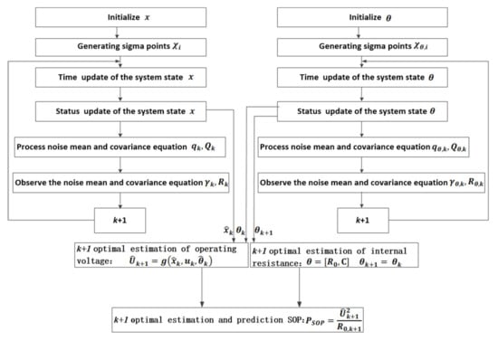
Figure 2.
SOP estimation flow chart.
5. Simulation and Discussion
5.1. SOE Estimation Based on ADUKF
According to Figure 3, an EULB (as shown in Table 1) was selected to conduct the charge/discharge experiment using test equipment (BTS20, 5V/4*300A/WD, Hubei Techpow Electric Co., Ltd., Xiangfan, China) at room temperature. In order to simulate the working conditions, the fully charged EULB was discharged several times. Different discharge currents were used each time for simulation verification and analysis based on MATLAB R2021a (MathWorks, Natick, MA, USA).
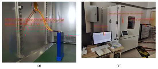
Figure 3.
Battery testing system. (a) The lithium iron echelon-use battery. (b) The charge/discharge experiment.

Table 1.
Parameters of the EULB.
In order to verify the adaptive characteristics of the ADUKF algorithm, a test experiment was carried out on a fully charged EULB, starting from SOE of 100% and ending at SOE of 25%. In the paper, selected battery symmetry capacity decays to 80%, 60%, 40%, and 20% separately of rated capacity, and the initial SOE values were changed to 70% and 40% separately, and the adaptive and error curves were observed and analyzed.
In the process of simulation verification, the estimated values of SOE, working voltage, and SOP were calculated based on the ADUKF algorithm, and the actual values were acquired by the test equipment (BTS20).
The formula for error is as follows:
According to Equations (1), (2) and (24), , is the optimal value of SOE.
The SOE error equation is as follows:
where, is the value collected by the device.
According to Equation (29), the optimal estimation of the working voltage is at time k + 1.
The working voltage error equation is as follows:
where is the value acquired by the test equipment.
According to Equation (31), the optimal estimation SOP is at time k + 1.
The SOP error equation is as follows:
where, is the value acquired by the test equipment.
5.2. Capacity Decays to 80% and SOE Starts at 70%
The simulation verification curve when capacity decays to 80% and SOE starts at 70% is shown in Figure 4.
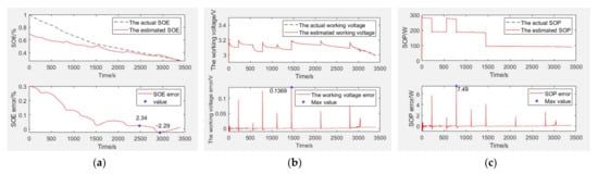
Figure 4.
The simulation verification curve when capacity decays to 80% and SOE starts at 70%. Estimation and error curves of (a) SOE, (b) working voltage, and (c) SOP.
SOE estimation curves of EULB are shown in Figure 4a, the bottom graph is the SOE error curve and the top graph is the SOE adaptive estimation curve. As shown in Table 2, the SOE error is −2.29% to 2.34%, and SOE estimation is adaptive through curve comparison.
Table 2.
Estimation error of the EULB’s parameters.
The working voltage estimation curves of EULB are shown in Figure 4b, the bottom graph is the working voltage error curve and the top graph is the working voltage adaptive estimation curve. As shown in Table 2, the working voltage error is 0.1369 V (within 4.28%), and the working voltage estimation is adaptive through curve comparison.
5.3. Capacity Decays to 80% and SOE Starts at 40%
The simulation verification curve when capacity decays to 80% and SOE starts at 40% is shown in Figure 5.
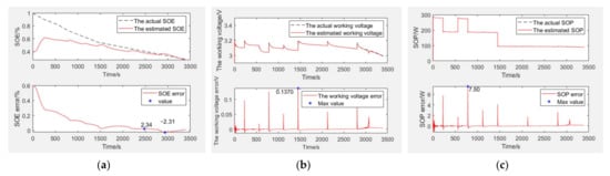
Figure 5.
The simulation verification curve when capacity decays to 80% and SOE starts at 40%. Estimation and error curves of (a) SOE, (b) working voltage, and (c) SOP.
SOE estimation curves of the EULB are shown in Figure 5a, the bottom graph is the SOE error curve and the top graph is the SOE adaptive estimation curve. As shown in Table 2, the SOE error is −2.31% to 2.34%, and SOE estimation is adaptive through curve comparison.
The working voltage estimation curves of the EULB are shown in Figure 5b, the bottom graph is the working voltage error curve and the top graph is the working voltage adaptive estimation curve. As shown in Table 2, the working voltage error is 0.1370 V (within 4.28%), and the working voltage estimation is adaptive through curve comparison.
5.4. Capacity Decays to 60% and SOE Starts at 70%
The simulation verification curve when capacity decays to 60% and SOE starts at 70% in Figure 6.
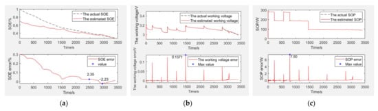
Figure 6.
The simulation verification curve when capacity decays to 60% and SOE starts at 70%. Estimation and error curves of (a) SOE, (b) working voltage, and (c) SOP.
SOE estimation curves of the EULB are shown in Figure 6a, the bottom graph is the SOE error curve and the top graph is the SOE adaptive estimation curve. As shown in Table 2, the SOE error is −2.23% to 2.35%, and SOE estimation is adaptive through curve comparison.
The working voltage estimation curves of EULB are shown in Figure 6b, the bottom graph is the working voltage error curve and the top graph is the working voltage adaptive estimation curve. As shown in Table 2, the working voltage error is 0.1371 V (within 4.28%), and the working voltage estimation is adaptive through curve comparison.
5.5. Capacity Decays to 60% and SOE Starts at 40%
The simulation verification curve when capacity decays to 60% and SOE starts at 40% in Figure 7.
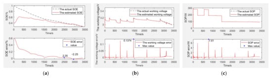
Figure 7.
The simulation verification curve when capacity decays to 60% and SOE starts at 40%. Estimation and error curves of (a) SOE, (b) working voltage, and (c) SOP.
SOE estimation curves of the EULB are shown in Figure 7a, the bottom graph is the SOE error curve and the top graph is the SOE adaptive estimation curve. As shown in Table 2, the SOE error is −2.25% to 2.35%, and SOE estimation is adaptive through curve comparison.
The working voltage estimation curves of the EULB are shown in Figure 7b, the bottom graph is the working voltage error curve and the top graph is the working voltage adaptive estimation curve. As shown in Table 2, the working voltage error is 0.1374 V (within 4.29%), and the working voltage estimation is adaptive through curve comparison.
5.6. Capacity Decays to 40% and SOE Starts at 70%
The simulation verification curve when capacity decays to 40% and SOE starts at 70% is shown in Figure 8.
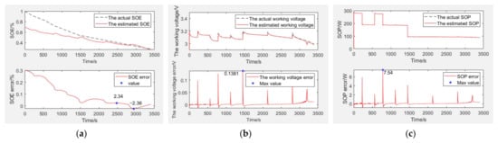
Figure 8.
The simulation verification curve when capacity decays to 40% and SOE starts at 70%. Estimation and error curves of (a) SOE, (b) working voltage, and (c) SOP.
SOE estimation curves of the EULB are shown in Figure 8a, the bottom graph is the SOE error curve and the top graph is the SOE adaptive estimation curve. As shown in Table 2, the SOE error is −2.36% to 2.34%, and SOE estimation is adaptive through curve comparison.
The working voltage estimation curves of the EULB are shown in Figure 8b, the bottom graph is the working voltage error curve and the top graph is the working voltage adaptive estimation curve. As shown in Table 2, the working voltage error is 0.1381 V (within 4.32%), and the working voltage estimation is adaptive through curve comparison.
5.7. Capacity Decays to 40% and SOE Starts at 40%
The simulation verification curve when capacity decays to 40% and SOE starts at 40% is shown in Figure 9.
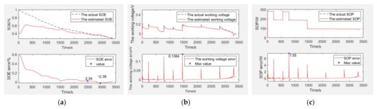
Figure 9.
The simulation verification curve when capacity decays to 40% and SOE starts at 40%. Estimation and error curves of (a) SOE, (b) working voltage, and (c) SOP.
SOE estimation curves of the EULB are shown in Figure 9a, the bottom graph is the SOE error curve and the top graph is the SOE adaptive estimation curve. As shown in Table 2, the SOE error is −2.38% to 2.34%, and SOE estimation is adaptive through curve comparison.
The working voltage estimation curves of the EULB are shown in Figure 9b, the bottom graph is the working voltage error curve and the top graph is the working voltage adaptive estimation curve. As shown in Table 2, the working voltage error is 0.1384 V (within 4.33%), and the working voltage estimation is adaptive through curve comparison.
5.8. Capacity Decays to 20% and SOE Starts at 70%
The simulation verification curve when capacity decays to 20% and SOE starts at 70% is shown in Figure 10.
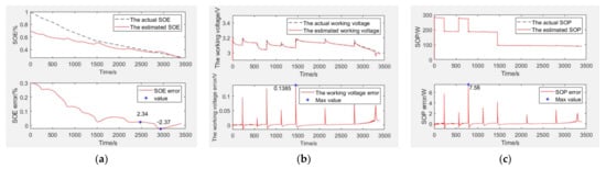
Figure 10.
The simulation verification curve when capacity decays to 20% and SOE starts at 70%. Estimation and error curves of (a) SOE, (b) working voltage, and (c) of SOP.
SOE estimation curves of the EULB are shown in Figure 10a, the bottom graph is the SOE error curve and the top graph is the SOE adaptive estimation curve. As shown in Table 2, the SOE error is −2.37% to 2.34%, and SOE estimation is adaptive through curve comparison.
The working voltage estimation curves of the EULB are shown in Figure 10b, the bottom graph is the working voltage error curve and the top graph is the working voltage adaptive estimation curve. As shown in Table 2, the working voltage error is 0.1385 V (within 4.33%), and the working voltage estimation is adaptive through curve comparison.
5.9. Capacity Decays to 20% and SOE Starts at 40%
The simulation verification curve when capacity decays to 20% and SOE starts at 40% is shown in Figure 11.
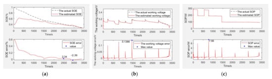
Figure 11.
The simulation verification curve when capacity decays to 20% and SOE starts at 40%. Estimation and error curves of (a) SOE, (b) working voltage, and (c) SOP.
SOE estimation curves of the EULB are shown in Figure 11a, the bottom graph is the SOE error curve and the top graph is the SOE adaptive estimation curve. As shown in Table 2, the SOE error is −2.39% to 2.34%, and SOE estimation is adaptive through curve comparison.
The working voltage estimation curves of the EULB are shown in Figure 11b, the bottom graph is the working voltage error curve and the top graph is the working voltage adaptive estimation curve. As shown in Table 2, the working voltage error is 0.1386 V (within 4.33%), and the working voltage estimation is adaptive through curve comparison.
SOP estimation curves of the EULB are shown in Figure 11c, the bottom graph is the SOP error curve and the top graph is SOP adaptive estimation curve. As shown in Table 2, the SOP error is 7.56 W (within 3.28%), and SOP estimation is adaptive through curve comparison.
Simulation results show that the estimation accuracy error of the EULB’s SOE is less than 2.38%, that the EULB working voltage is less than 4.33%, and that the EULB’s SOP is less than 3.28%. The method is adaptive regardless of whether the initial SOE value is consistent with the actual value.
6. Conclusions
In this paper, the SRCSEM of an EULB is established first, and then the SOP estimation method of such a battery is established based on the ADUKF algorithm. Simulation shows that, at the same degradation level, the greater the initial SOE error, the greater the error of SOP estimation, the more serious the degradation level of the battery, and the greater the error of estimation of SOE, operating voltage, and SOP. Simulation results show that the estimation accuracy error of the EULB’s SOP is less than 3.28%. The accuracy is higher than reference [23] and lower than reference [24]; thus, the method has high accuracy. Furthermore, regardless of whether the initial value of the SOE is clear or not, the ADUKF algorithm can be adjusted to an adaptive algorithm.
Therefore, on the basis of ensuring estimation accuracy, the adaptive ability of the SOP estimation method is enhanced.
Author Contributions
Conceptualization, Y.X. and E.H.; methodology, Y.X.; software, E.H.; validation, E.H., Y.X. and X.Q.; formal analysis, G.L.; investigation, G.L.; resources, Y.X.; data curation, E.H.; writing—original draft preparation, E.H.; writing—review and editing, Y.X.; visualization, X.Q.; supervision, Y.X.; project administration, Z.W.; funding acquisition, Y.X. All authors have read and agreed to the published version of the manuscript.
Funding
This work was supported by the Science and Technology Major Project of Inner Mongolia Autonomous Region (2020ZD0014).
Institutional Review Board Statement
Not applicable.
Informed Consent Statement
Not applicable.
Data Availability Statement
Not applicable.
Acknowledgments
This research was conducted within the University of Shandong Jiao Tong, supported by the charging-discharging equipment (BTS20-5V/4*300A/WD). We are thankful to the testing and simulation team members for their support with the experiment.
Conflicts of Interest
The authors declare no conflict of interest.
Abbreviations
The following abbreviations are most common in this manuscript:
| EULB | Echelon-use lithium-ion battery |
| AUKF | Adaptive unscented Kalman filter |
| SRCSEM | Second-order resistor-capacitance symmetry equivalent model |
| SOC | State of charge |
| SOH | State of health |
| SOP | State of power |
| SOE | State of energy |
| OCV | Open circuit voltage |
| ADUKF | Adaptive dual unscented Kalman filter |
| UT | Unscented transformation |
| EVs | Electric vehicles |
| UKF | Unscented Kalman filter |
| USABC | United States Advanced Battery Consortium |
References
- Neubauer, J.; Ahmad, P. The ability of battery second use strategies to impact plug-in electric vehicle prices and serve utility energy storage applications. J. Power Sources 2011, 196, 10351–10358. [Google Scholar] [CrossRef]
- Tong, S.J.; Same, A.; Kootstra, M.A.; Park, J.W. Off-grid photovoltaic vehicle charge using second life lithium batteries: An experimental and numerical investigation. Appl. Energy 2013, 104, 740–750. [Google Scholar] [CrossRef]
- Omar, N.; Daowd, M. Assessment of second life of lithium iron phosphate-based batteries. Int. Rev. Electr. Eng. (IREE) 2012, 7, 3941–3948. [Google Scholar]
- Jiang, Y.; Jiang, J.; Zhang, C.; Zhang, W.; Gao, Y.; Li, N. State of health estimation of second-life LiFePO4 batteries for energy storage applications. J. Clean. Prod. 2018, 205, 754–762. [Google Scholar] [CrossRef]
- Simon, F.S.; Martin, J.B.; Christian, C.; Markus, G.; Andreas, J. Correlation between capacity and impedance of lithium-ion cells during calendar and cycle life. J. Power Sources 2016, 305, 191–199. [Google Scholar] [CrossRef]
- Zhang, Y.; Li, Y.; Tao, Y.; Ye, J.; Pan, A.; Li, X.; Liao, Q.; Wang, Z. Performance assessment of retired EV battery modules for echelon use. Energy 2020, 993, 116555. [Google Scholar] [CrossRef]
- Hunt, G. USABC Electric Vehicle Battery Test Procedures Manual. Revision 2; Technical Reports; Office of Scientific & Technical Information: Washington, DC, USA, 1996.
- Wik, T.; Fridholm, B.; Kuusisto, H. Implementation and Robustness of an Analytically Based Battery State of Power. J. Power Sources 2015, 287, 448–457. [Google Scholar] [CrossRef]
- Li, F. Test Method for Peak Output Power of Nickel Metal Hydride Power Batteries. Master’s Thesis, Central South University, Changsha, China, 2007. [Google Scholar]
- Hu, Y. Prediction Status of Peak Power of Battery on HEV. Master’s Thesis, Harbin Institute of Technology, Harbin, China, 2012. [Google Scholar]
- Plett, G.L. High-performance Battery-pack Power Estimation using a Dynamic Cell Model. IEEE Trans. Veh. Technol. 2004, 53, 1586–1593. [Google Scholar] [CrossRef] [Green Version]
- Wang, S.; Verbrugge, M.; Wang, J.S. Power Prediction from a Battery State Estimator that Incorporates Diffusion Resistance. J. Power Sources 2012, 214, 399–406. [Google Scholar] [CrossRef]
- Wang, S.; Verbrugge, M.; Wang, J.S. Multi-parameter Battery State Estimator Based on the Adaptive and Direct Solution of the Governing Differential Equations. J. Power Sources 2011, 196, 8735–8741. [Google Scholar] [CrossRef]
- Zhou, W.; Zhang, N.; Zhai, H. Enhanced Battery Power Constraint Handling in MPC-Based HEV Energy Management: A Two-Phase Dual-Model Approach. IEEE Trans. Transp. Electrif. 2021, 7, 1236–1248. [Google Scholar] [CrossRef]
- Zhang, T.; Guo, N.; Sun, X.; Fan, J.; Yang, N.; Song, J. A Systematic Framework for State of Charge, State of Health and State of Power Co-Estimation of Lithium-Ion Battery in Electric Vehicles. Sustainability 2021, 13, 5166. [Google Scholar] [CrossRef]
- Lin, P.; Wang, Z.; Jin, P.; Hong, J. Novel Polarization Voltage Model: Accurate Voltage and State of Power Prediction. IEEE Access 2020, 8, 92039–92049. [Google Scholar] [CrossRef]
- Lu, J.; Chen, Z.; Yang, Y.; Lv, M. Online Estimation of State of Power for Lithium-Ion Batteries in Electric Vehicles Using Genetic Algorithm. IEEE Access 2018, 6, 20868–20880. [Google Scholar] [CrossRef]
- Nejad, S.; Gladwin, D.T.; Stone, D.A. On-chip implementation of Extended Kalman Filter for adaptive battery states monitoring. In Proceedings of the IECON 2016—42nd Annual Conference of the IEEE Industrial Electronics Society, Florence, Italy, 23–26 October 2016; pp. 5513–5518. [Google Scholar] [CrossRef] [Green Version]
- Nejad, S.; Gladwin, D.T. Online Battery State of Power Prediction Using PRBS and Extended Kalman Filter. IEEE Trans. Ind. Electron. 2020, 67, 3747–3755. [Google Scholar] [CrossRef]
- Chen, Z.; Lu, J.; Yang, Y.; Xiong, R. Online estimation of state of power for lithium-ion battery considering the battery aging. In Proceedings of the 2017 Chinese Automation Congress (CAC), Jinan, China, 20–22 October 2017; pp. 3112–3116. [Google Scholar] [CrossRef]
- Shrivastava, P.; Soon, T.K.; Idris, M.Y.I.B.; Mekhilef, S. Overview of Model-Based Online State-of-Charge Estimation Using Kalman Filter Family for Lithium-Ion Batteries. Renew. Sustain. Energy Rev. 2019, 113, 109233. [Google Scholar] [CrossRef]
- Cheng, W.; Yi, Z.; Liang, J.; Song, Y.; Liu, D. An SOC and SOP Joint Estimation Method of Lithium-ion Batteries in Unmanned Aerial Vehicles. In Proceedings of the 2020 International Conference on Sensing, Measurement & Data Analytics in the Era of Artificial Intelligence (ICSMD), Xi’an, China, 5–17 October 2020; pp. 247–252. [Google Scholar] [CrossRef]
- Hou, E.; Xu, Y.; Qiao, X.; Liu, G.; Wang, Z. State of Power Estimation of Echelon-Use Battery Based on Adaptive Dual Extended Kalman Filter. Energies 2021, 14, 5579. [Google Scholar] [CrossRef]
- Shrivastava, P.; Soon, T.K.; Idris, M.Y.I.B.; Mekhilef, S.; Adnan, S.B.R.S. Model-based state of X estimation of lithium-ion battery for electric vehicle applications. Int. J. Energy Res. 2022, 1–20. [Google Scholar] [CrossRef]
- Rahimifard, S.; Ahmed, R.; Habibi, S. Interacting Multiple Model Strategy for Electric Vehicle Batteries State of Charge/Health/Power Estimation. IEEE Access 2021, 9, 109875–109888. [Google Scholar] [CrossRef]
- Lin, P.; Jin, P.; Hong, J.; Wang, Z. Battery voltage and state of power prediction based on an improved novel polarization voltage model. Energy Rep. 2020, 6, 2299–2308. [Google Scholar] [CrossRef]
- Liu, C.; Hu, M.; Jin, G.; Xu, Y.; Zhai, J. State of power estimation of lithium-ion battery based on fractional-order equivalent circuit model. J. Energy Storage 2021, 41, 102954. [Google Scholar] [CrossRef]
- Hou, E.; Qiao, X.; Liu, G. Modeling and Simulation of Power Lithium-ion Battery SOC. Chin. Comput. Simul. 2014, 31, 193–196. [Google Scholar]
- Yi, F.; Lu, D.; Wang, X.; Pan, C.; Tao, Y.; Zhou, J.; Zhao, C. Energy Management Strategy for Hybrid Energy Storage Electric Vehicles Based on Pontryagin’s Minimum Principle Considering Battery Degradation. Sustainability 2022, 14, 1214. [Google Scholar] [CrossRef]
- Hou, E.; Qiao, X.; Liu, G.; Li, Y. Influence of temperature on parameters of power lithium-ion battery based on RC equivalent circuit. Chin. J. Power Sources 2015, 39, 287–289. [Google Scholar]
- Cao, L.; Huang, J.; Cao, M.; Yang, K. SOC and internal resistance estimation of lithium battery based on DKF. J. Nanchang Univ. Eng. Technol. 2018, 40, 179–183. [Google Scholar]
- Hou, E.; Qiao, X.; Liu, G. Estimation of power lithium-ion battery SOC based on fuzzy optimal decision. Chin. J. Power Sources 2017, 41, 920–922. [Google Scholar]
- Shi, J.; Li, B.; Liu, M.F. Study on degenerate of lithium-ion battery based on fuzzy inference system. Chin. J. Power Sources 2018, 42, 1488–1490. [Google Scholar]
- Gu, Y.; Zhang, Y. SOC Estimation of Lithium Battery Based on Double Kalman Filter. Chin. J. Power Sources 2016, 40, 986–989. [Google Scholar]
- Liu, X.; He, Y.; Zeng, G.J. Power State Estimation of Lithium Battery Considering Temperature Effect. Chin. J. Power Technol. 2016, 31, 155–163. [Google Scholar]
- She, L.Y. Research on Joint Estimation of SOC and SOP for Vehicle Power Battery. Master’s Thesis, Wuhan University of Technology, Wuhan, China, 2018. [Google Scholar]
- Peng, S.; Zhu, X.; Xing, Y.; Shi, H.; Cai, X.; Pecht, M. An adaptive state of charge estimation approach for lithium-ion series-connected battery system. J. Power Sources 2018, 392, 48–59. [Google Scholar] [CrossRef]
- Zhang, S.; Guo, X.; Zhang, X. An improved adaptive unscented kalman filtering for state of charge online estimation of lithium-ion battery. J. Energy Storage 2020, 32, 101980. [Google Scholar] [CrossRef]
- Li, Y.; Yuan, M.; Chadli, M.; Wang, Z.; Zhao, D. Unknown input functional observer design for discrete time interval type-2 Takagi-Sugeno fuzzy systems. IEEE Trans. Fuzzy Syst. 2022. [Google Scholar] [CrossRef]
- Lin, X.; Tang, Y.; Ren, J.; Wei, Y. State of charge estimation with the adaptive unscented Kalman filter based on an accurate equivalent circuit model. J. Energy Storage 2021, 41, 102840. [Google Scholar] [CrossRef]
- Li, Y.; Liu, S.; Zhao, D.; Shi, X.; Cui, Y. Event-triggered fault estimation for discrete time-varying systems subject to sector-bounded nonlinearity: A Krein space-based approach. Int. J. Robust Nonlinear Control 2021, 31, 5360–5380. [Google Scholar] [CrossRef]
Publisher’s Note: MDPI stays neutral with regard to jurisdictional claims in published maps and institutional affiliations. |
© 2022 by the authors. Licensee MDPI, Basel, Switzerland. This article is an open access article distributed under the terms and conditions of the Creative Commons Attribution (CC BY) license (https://creativecommons.org/licenses/by/4.0/).