
Estimation of Symmetry in the Recognition System with Adaptive Application of Filters


1
Department of Automated Control Systems, Lviv Polytechnic National University, 79013 Lviv, Ukraine
2
Department of Information Technology Publishing, Lviv Polytechnic National University, 79013 Lviv, Ukraine
*
Author to whom correspondence should be addressed.
Symmetry 2022, 14(5), 903; https://doi.org/10.3390/sym14050903
Submission received: 16 February 2022
/
Revised: 24 March 2022
/
Accepted: 28 March 2022
/
Published: 28 April 2022
(This article belongs to the Topic Applied Metaheuristic Computing)
Abstract
:The aim of this work is to study the influence of lighting on different types of filters in order to create adaptive systems of perception in the visible spectrum. This problem is solved by estimating symmetry operations (operations responsible for image/image transformations). Namely, the authors are interested in an objective assessment of the possibility of reproducing the image of the object (objective symmetry of filters) after the application of filters. This paper investigates and shows the results of the most common edge detection filters depending on the light level; that is, the behavior of the system in a room with indirect natural and standard (according to the requirements of the educational process in Ukraine) electric lighting was studied. The methods of Sobel, Sobel x, Sobel y, Prewitt, Prewitt x, Prewitt y, and Canny were used and compared in experiments. The conclusions provide a subjective assessment of the performance of each of the filters in certain conditions. Dependencies are defined that allow giving priority to certain filters (from those studied) depending on the lighting.
1. Introduction
In the last decade, the possibilities of autonomous decision making by computer vision systems have been actively studied. The topic of autonomous agents to support solutions that are able to adapt to the environment is relevant in a variety of applications: medicine [1,2,3], systems and means of artificial intelligence [4,5,6]. The problem includes the question of where fuzzy logic is needed [7], security issues [8,9,10,11] and biometric recognition systems [12,13], systems to support people with disabilities and related technologies and applications aimed to include wayfinding and navigation [5,13], land research, space research, agricultural issues, industrial climate issues, smart things, etc.
The task of automated selection of key characteristics for the classification of images using computer tools is not a trivial problem [14,15,16]; especially for the variable field of attention [17,18]. There are many methods and algorithms for identifying key characteristics for image classification [19,20,21,22,23,24], but each has its disadvantages and advantages. Most of the existing methods that solve this problem are effective only for individual objects, such as human faces, simple geometric shapes, and handwritten or printed symbols, but only under certain conditions, including certain lighting and the position of the object from the wearable camera and background. An urgent problem now is the creation of automated systems that compensate for the limited capabilities of people at different levels. When using artificial neural networks [19,20], reducing the amount of computation in learning is an important element to teach mathematical options for processing. This paper considers the problem of comparing the methods of selection of characteristic features under different external conditions in order to identify the best method for given conditions. Adaptive algorithms for detecting, classifying, and tracking the edges of objects have been developed in [25]. Adaptation is achieved by using thresholds to obtain contours. The creation of contours is achieved through the Kalman filter, the use of which significantly improves the computation time, as well as provides the system with the required accuracy. In [26], invariant approaches to structural features were used to find facial features, texture, shape, and color of the skin regardless of changes in lighting. Statistical models have been developed, which are the basis for testing the model. The advantage of the proposed method is that it can detect faces of different sizes and different poses without restrictions on lighting conditions. However, the spectral characteristics of the face / skin are not studied in this work. In [27], for an image that is under background and lighting conditions, a method for determining the edges based on the advanced arithmetic operator Prewitt was proposed. An improved preprocessing operation was performed in the work. The characteristics of horizontal projection and vertical location of the upper and lower edges for positioning were used. The results of the experiments show that the algorithm has high speed, positioning speed, and good practical value.
Table 1 shows the increase in absolute contrast values from the state of the object. The state of the object can change tens of thousands of times, and up to one million times when exposed to the sun. Because glare affects the brightness of an object, the brightness of the sun’s disk can reach up to 108 lux. Shade illumination can be reduced to 100 lux. Today, it is impossible to observe several objects with tens of thousands of different illuminations on the same camera. Therefore, the inevitable loss of information.
The aim of the work is to create adaptive systems of perception in the visible spectrum by constructing the dependences of the quality of the applied filters in dynamically changing conditions. In particular, the paper studies the behavior (in terms of symmetry of object representation) of the most popular methods of detecting edges under different lighting conditions.
2. Materials and Methods
2.1. Sobel’s Operator
The Sobel operator is a discrete differential operator that calculates the approximate value of the image gradient [28]. The result of the application of the Sobel operator at each point of the image is either the brightness gradient vector at this point or its norms.
2.1.1. Description
The image convolution on which the Sobel operator is based is performed by small separable integer filters in the vertical and horizontal directions. The Sobel operator uses a gradient approximation that is not accurate, and this becomes especially noticeable at high-frequency image oscillations.
At each point of the image, the brightness gradient is calculated by the Sobel operator. Thus, there is the direction of the greatest increase in brightness and change of this value. Changing the brightness indicates the smoothness or sharpness of the change at each point of the image, the probability of finding a point on the border, and hence the orientation of the contour. This calculation is more reliable and simpler than calculating the direction of orientation.
A two-dimensional vector is a gradient of the function of two variables for each point of the image. Its components are derivatives of image brightness, which are calculated horizontally and vertically. The result of the work of the Sobel operator will be a zero vector at the point of the region of constant brightness and at the point lying on the boundary of the regions, a vector with the direction of increasing brightness.
2.1.2. Formulation
Strictly speaking, the operator uses 3 × 3 cores to calculate output values. If A is the original image, and Gx and Gy are two images with approximate points of derivatives in x and y:
where ∗ means a two-dimensional convolution operation.
The x-coordinate here increases “to the right”, and y “down”. At each point of the image, the approximate value of the gradient value can be calculated using the obtained approximate values of the derivatives (meaning element by element):
Using this information, we can also calculate the direction of the gradient:
where, for example, the angle Θ is zero for the vertical boundary in which the dark side is on the left.
The brightness function is known to us at discrete points, we need to determine the differentiated function that passes through these points. Derivatives at any single point are functions of brightness from all points of the image. The solution of the derivatives can be calculated with a certain degree of accuracy.
Sobel’s operator is an inaccurate approximation of the image gradient, but it is high enough for practical application in many problems. Specifically, the operator uses the intensity value only around 3 × 3 of each pixel to obtain an approximation of the corresponding image gradient and uses only integer values of the luminance weights to estimate the gradient.
2.1.3. Extension to Another Number of Dimensions
The Sobel operator consists of two separate operations:
- Smoothing with a triangular filter perpendicular to the derivative direction:
- Finding a simple central change in the direction of the derivative:
Sobel filters for image derivatives in various dimensions for
Here is an example of a three-dimensional Sobel core for an axis z:
2.1.4. Technical Details
As follows from the definition, the Sobel operator can be implemented by simple hardware and software. Approximating the vector gradient requires only eight pixels around point x of the image and integer arithmetic. Moreover, both discrete filters described above can be separated:
and two derivatives, Gx and Gy, can now be calculated as
The resolution of these calculations can reduce the arithmetic operations with each pixel.
2.2. Canny’s Operator
Canny’s operator (Canny boundary detector, Canny algorithm) is a computer vision detection operator in the field of computer vision. It was developed in 1986 by John F. Canny and uses a multistep algorithm to detect a wide range of boundaries in images [16,29]. Canny said that this filter could be well approximated by the first Gaussian derivative. Kenny introduced the concept of non-maximum suppression, which means that pixels of boundaries are declared pixels in which the local maximum of the gradient is reached in the direction of the gradient vector.
- Good detection (Kenny interpreted this property as increasing the signal-to-noise ratio);
- Good localization (correct determination of the edge position);
- A single response to one edge.
From these criteria, the target function of error cost was then built, the minimization of which is the “optimal” linear operator for convolution with images.
The boundary detector algorithm is not limited to calculating the gradient of the smoothed image. Only the maximum points of the image gradient remain in the border contour, and the maximum points lying near the border are removed. It also uses information about the direction of the border in order to remove the points right next to the border and not to break the border itself near the local gradient maxima. Then, with the help of two thresholds, weak borders are removed. The fragment of the border is processed as a whole. If the value of the gradient somewhere on the observed fragment exceeds the upper threshold; this fragment also remains on the “permissible” edge and in places where the value of the gradient falls below this threshold, until it falls below the lower threshold. If there is no point on the whole fragment with a value greater than the upper threshold, it is deleted. This hysteresis reduces the number of breaks in the original edges. The inclusion of noise attenuation in Kenny’s algorithm increases the stability of the results on the one hand and, on the other hand, increases computational costs and leads to distortion and even loss of boundary details. For example, this algorithm rounds the corners of objects and destroys boundaries at connection points.
The main stages of Canny’s algorithm are:
Smoothing: blurred images to remove noise. Canny’s operator uses a filter that may be close to the first Gaussian derivative σ = 1.4:
Search for gradients: borders are marked where the image gradient becomes maximum. They can have different directions, so Canny’s algorithm uses four filters to detect horizontal, vertical, and diagonal edges in a blurred image. At this stage, Formulas (2) and (3) are used.
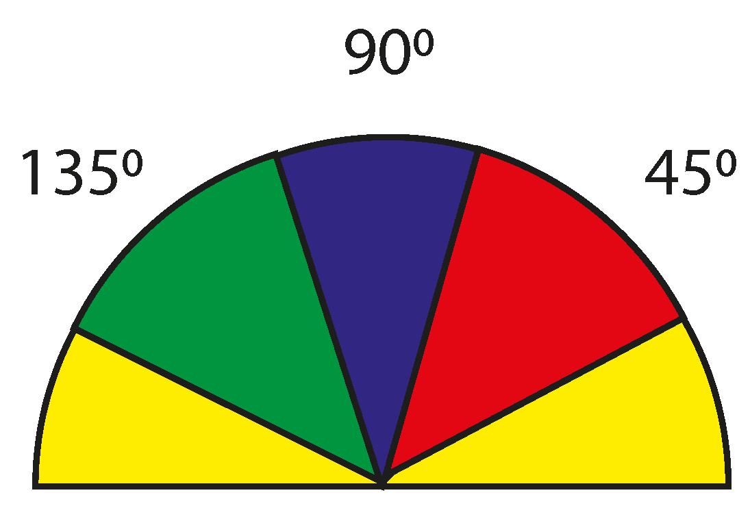
The angle of the direction of the gradient vector [30] is rounded and can take the following values: 0, 45, 90, and 135 (see Figure 1).
Suppression of non-maxima.
Only local maxima are marked as edges.
Double threshold filtering: potential limits are determined by thresholds.
Trace the area of ambiguity. The final limits are determined by suppressing all edges that are not related to certain (strong) limits.
Before using the detector, the image is usually converted to grayscale to reduce computational costs. This stage is typical of many image-processing methods.
2.3. Prewitt’s Operator
Prewitt operator is a method of selecting boundaries in image processing, which calculates the maximum response on the set of convolution cores to find the local orientation of the border in each pixel. It was created by Dr. Judith Prewitt to identify the boundaries of medical imaging [31].
Different kernels are used for this operation. From one core, you can obtain eight, rearranging the coefficients in a circle. Each result will be sensitive to the direction of the limit from 0 to 315 with a step of 45, where 0 corresponds to the vertical limit. The maximum response of each pixel is the value of the corresponding pixel in the original image. Its values are between 1 and 8, depending on the number of nuclei that provide the greatest result.
This method of edge detection is also called edge template matching because the image is mapped to a set of templates, and each represents some boundary orientation. The size and orientation of the border in a pixel is then determined by the pattern that best matches the local neighborhood of the pixel.
While a differential gradient detector requires a time-consuming calculation of the orientation estimate for magnitudes in the vertical and horizontal directions, the Prewitt limit detector provides a direct direction from the nucleus with maximum result. The set of nuclei is limited to 8 possible directions, but experience shows that most direct estimates of orientation are also not very accurate. On the other hand, a set of cores requires 8 convolutions for each pixel, while a set of gradients of the gradient method requires only 2: sensitive vertically and horizontally.
Formulation
The operator uses two 3 × 3 cores, collapsing the original image to calculate the approximate values of the derivatives: one horizontally and one vertically. Let A be the original image and Gx i Gy be two images in which each point contains a horizontal and vertical approximation of the derivative, which is calculated as:
3. Experiments
3.1. Experiment №1. 16:00, Action at 67–70 lux
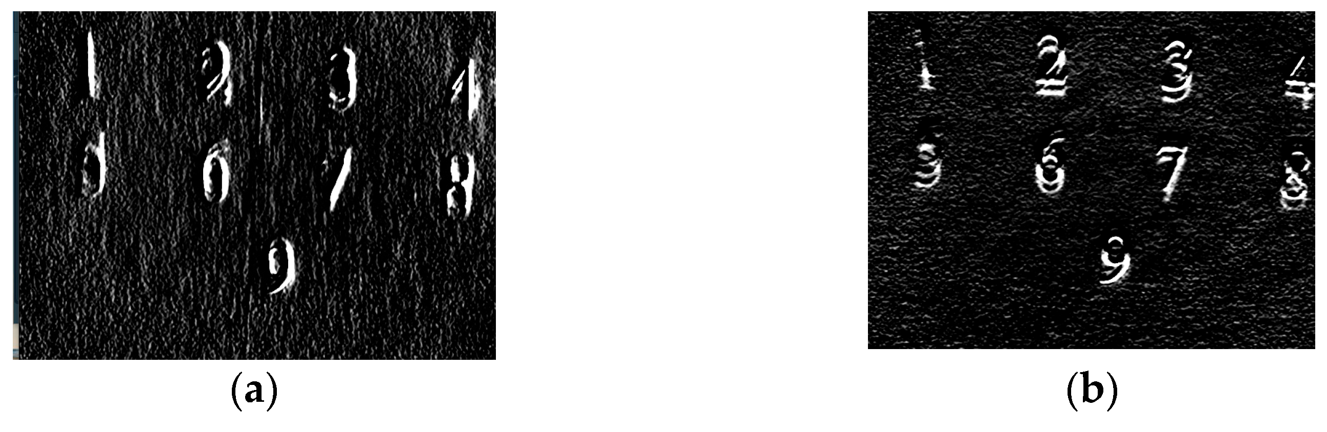
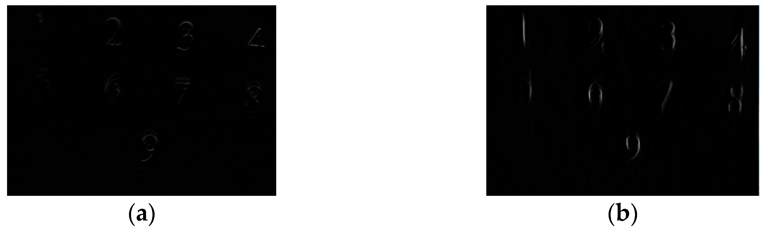
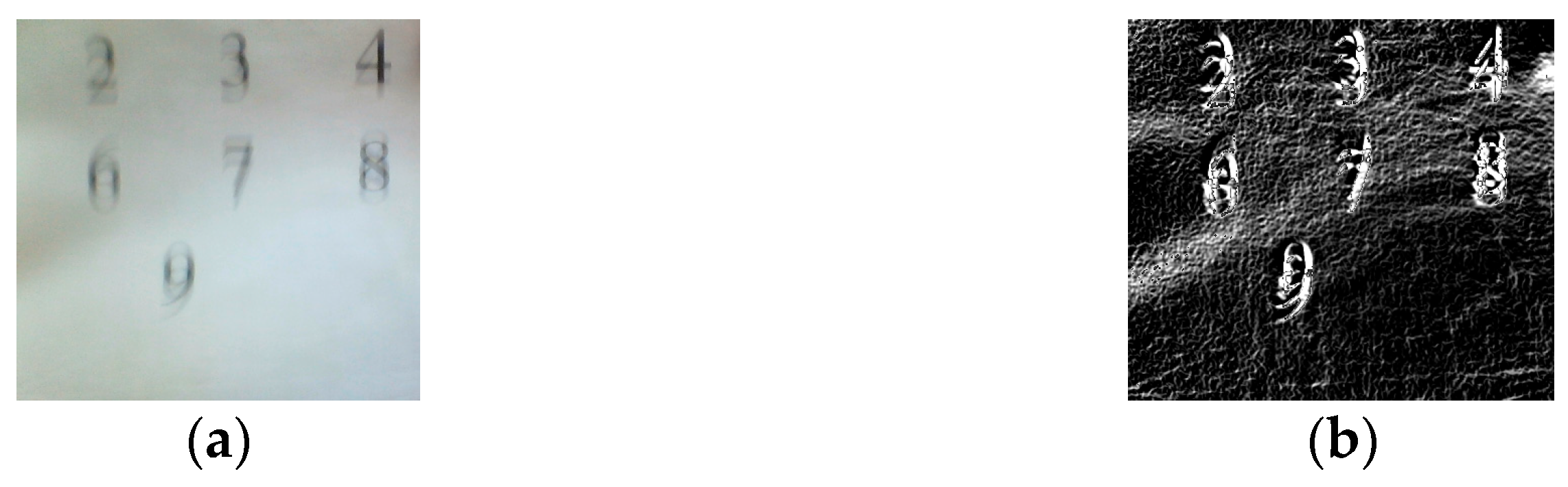
The program on the smartphone was used to measure the suites, as the study was performed to link to the most common video cameras. Figure 2, Figure 3, Figure 4, Figure 5, Figure 6, Figure 7, Figure 8, Figure 9, Figure 10, Figure 11, Figure 12, Figure 13, Figure 14, Figure 15, Figure 16, Figure 17, Figure 18, Figure 19, Figure 20, Figure 21, Figure 22, Figure 23, Figure 24, Figure 25, Figure 26, Figure 27, Figure 28 and Figure 29 shows the work of the considered methods in comparison with the original image. Images are grouped according to lighting conditions. Thus, the first experiment (lighting 70 lux) is presented in Figure 2 (original input image and the result of processing by the Sobel method); Figure 3 (normalized Sobel gradient on the X axis and gradient on the Y axis); Figure 4 (Canny and Pruitt method); Figure 5 (Prewitt’s operator on the X axis and (Prewitt’s operator on the Y axis).
3.2. Experiment №2. 16:30, Action at 50 Lux
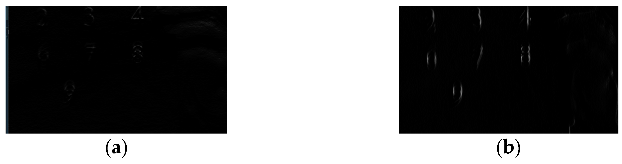
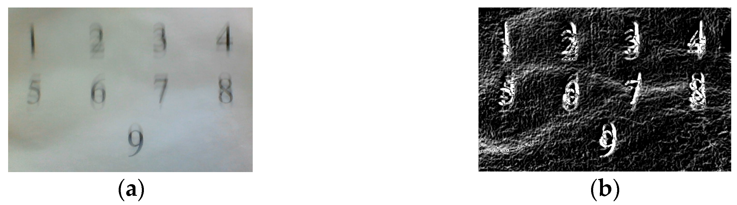
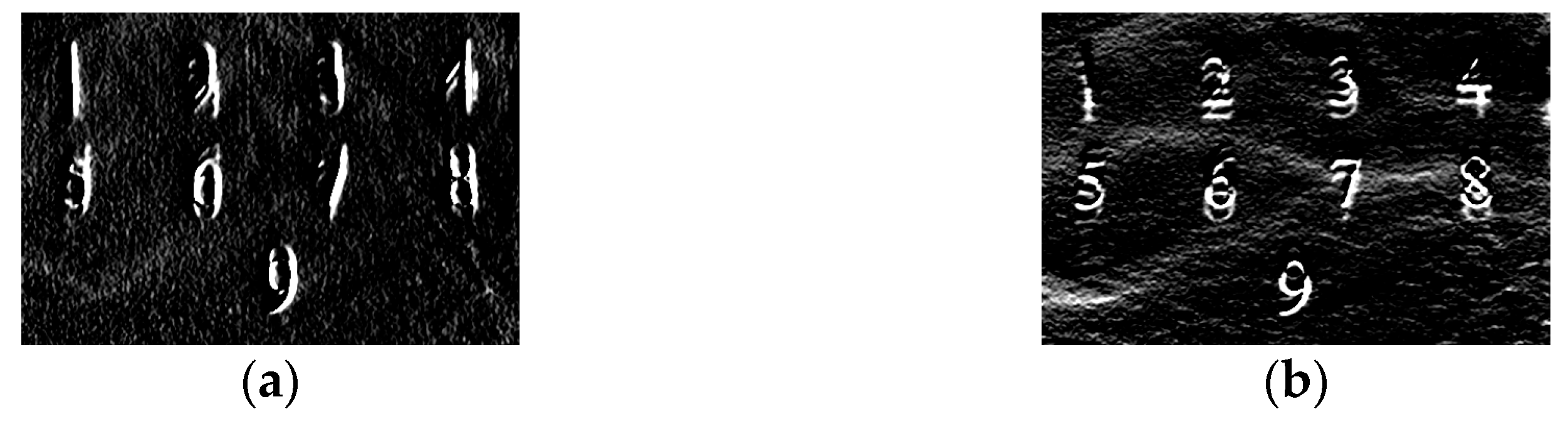
The second experiment (lighting 50 lux) is presented in Figure 6 (original input image and the result of processing by the Sobel method); Figure 7 (normalized Sobel gradient on the X-axis and gradient on the Y-axis); Figure 8 (Canny’s and Prewitt’s method); Figure 9 (Prewitt’s operator on the X-axis and (Prewitt’s operator on the Y-axis).
3.3. Experiment №3. 16:50, Action at 100 Lux (Includes E-Electric Lighting)
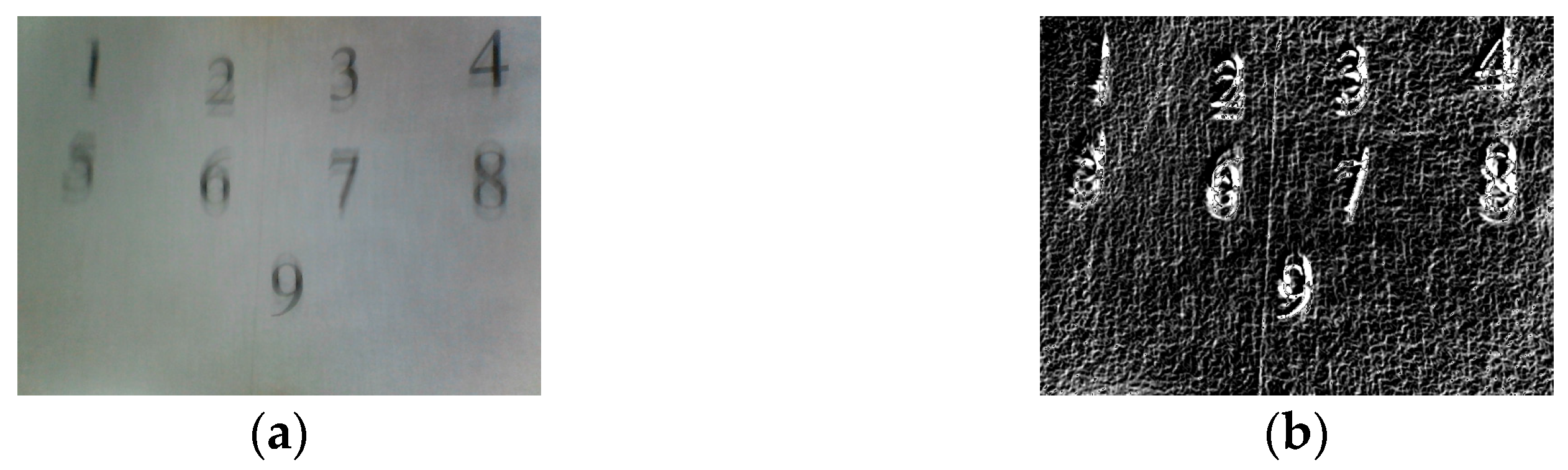
The third experiment (lighting 100 lux) is presented in Figure 10 (original input image and the result of processing by the Sobel method); Figure 11 (normalized Sobel gradient on the X-axis and gradient on the Y-axis); Figure 12 (Canny’s and Prewitt’s method); Figure 13 (Prewitt’s operator on the X-axis and (Prewitt’s operator on the Y-axis).
3.4. Experiment №3. 13:00, Action at 260 Lux
The forth experiment (lighting 260 lux) is presented in Figure 14 (original input image and the result of processing by the Sobel method); Figure 15 (normalized Sobel gradient on the X-axis and gradient on the Y-axis); Figure 16 (Canny’s and Prewitt’s method); Figure 17 (Prewitt’s operator on the X-axis and (Prewitt’s operator on the Y-axis).
3.5. Experiment №3. 13:30, Action at 2300 Lux
The fifth experiment (lighting 2300 lux) is presented in Figure 18 (original input image and the result of processing by the Sobel method); Figure 19 (normalized Sobel gradient on the X-axis and gradient on the Y-axis); Figure 20 (Canny’s and Prewitt’s method); Figure 21 (Prewitt’s operator on the X-axis and (Prewitt’s operator on the Y-axis).
3.6. Experiment №3. 13:30, Action at 2300 Lux + Man Shadow
The sixth experiment (lighting 2300 lux) is presented in Figure 22 (original input image and the result of processing by the Sobel method); Figure 23 (normalized Sobel gradient on the X-axis and gradient on the Y-axis); Figure 24 (Canny’s and Prewitt’s method); Figure 25 (Prewitt’s operator on the X-axis and (Prewitt’s operator on the Y-axis).
3.7. Experiment №3. 13:30, Action at 2350 Lux, Cam Front to Light
The seventh experiment (lighting 2350 lux) is presented in Figure 26 (original input image and the result of processing by the Sobel method); Figure 27 (normalized Sobel gradient on the X-axis and gradient on the Y-axis); Figure 28 (Canny’s and Prewitt’s method); Figure 29 (Prewitt’s operator on the X-axis and (Prewitt’s operator on the Y-axis).
4. Results
Figure 30 shows the dependences of the objective comparison of distances (PSNR) between the original value of the brightness of the pixel with the values obtained after applying the appropriate filters. The data in the chart are summarized.
The experiment was performed as follows. The original image was illuminated at 50 lux, 70 lux, 100, 260, and 2300 lux. These images are presented in Figure 2, Figure 6, Figure 10, Figure 14, Figure 18, Figure 22 and Figure 26, respectively. Canny, Sobel, and Prewitt filters were used for these images. These filtered images were compared with each other to assess the best performance of the filter and to make recommendations for the use of certain filters. Diagram 1 shows three graphs of the relationship between the signal-to-noise ratio of the filtered images. The blue color shows the values of the signal-to-noise ratio between img_sobel and img_sobel_x. This value takes the value of 7.23 and is the largest value in this chart, and therefore, they are the most similar to each other. The second value is the result of comparing img_sobel and img_sobel_y and takes the value of 6.92. We also observe high PSNR values compared to others, which explains that very similar transformations were used. The other values are a comparison between the pairs img_sobel and img_cany and img_sobel and img_prewitt_x, and img_sobel and img_prewitt_y. Because filtering was applied by other filters, the images are less similar, and that makes sense. Charts of other colors, similar to img_sobel_x and img_sobel_y, work similarly. Slightly higher values between the pairs img_sobel_x and img_prewitt_y are explained by the better finding of contours in the image, which should be taken into account when choosing one filtering method.
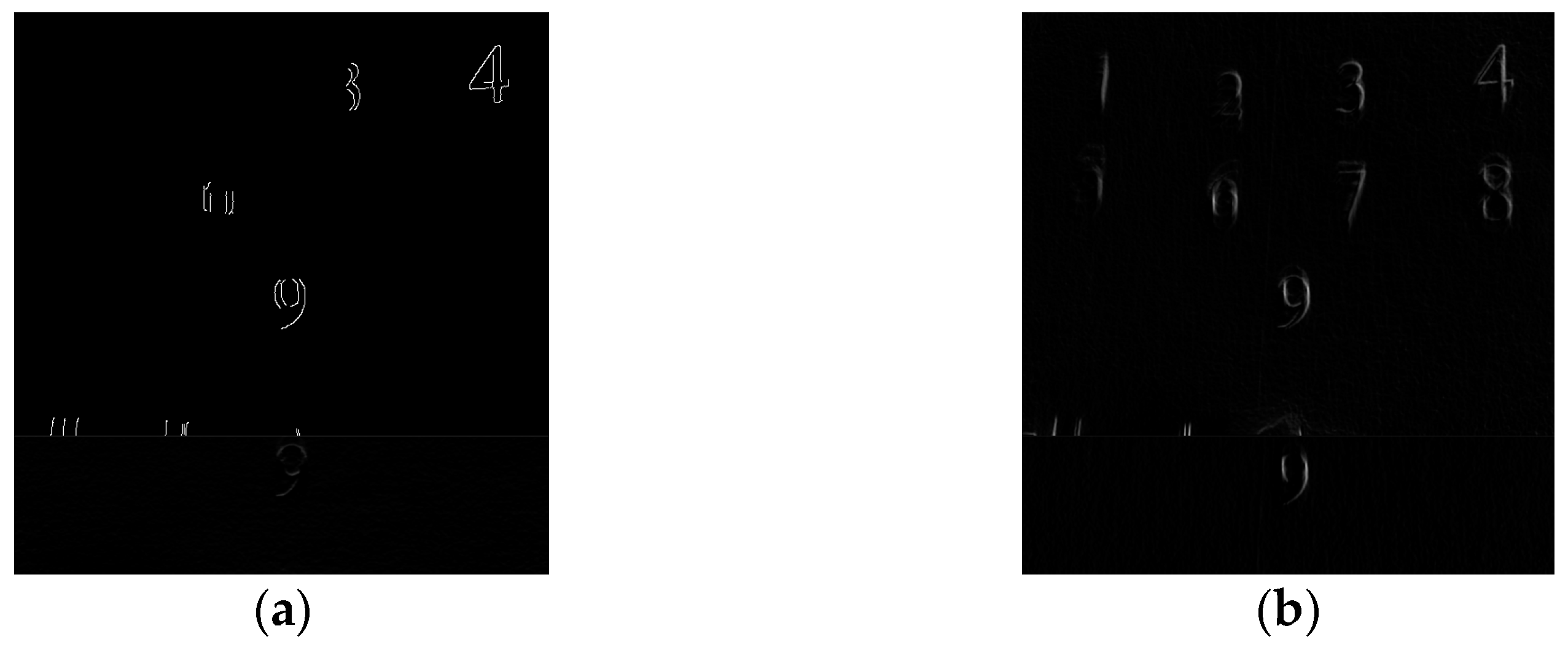
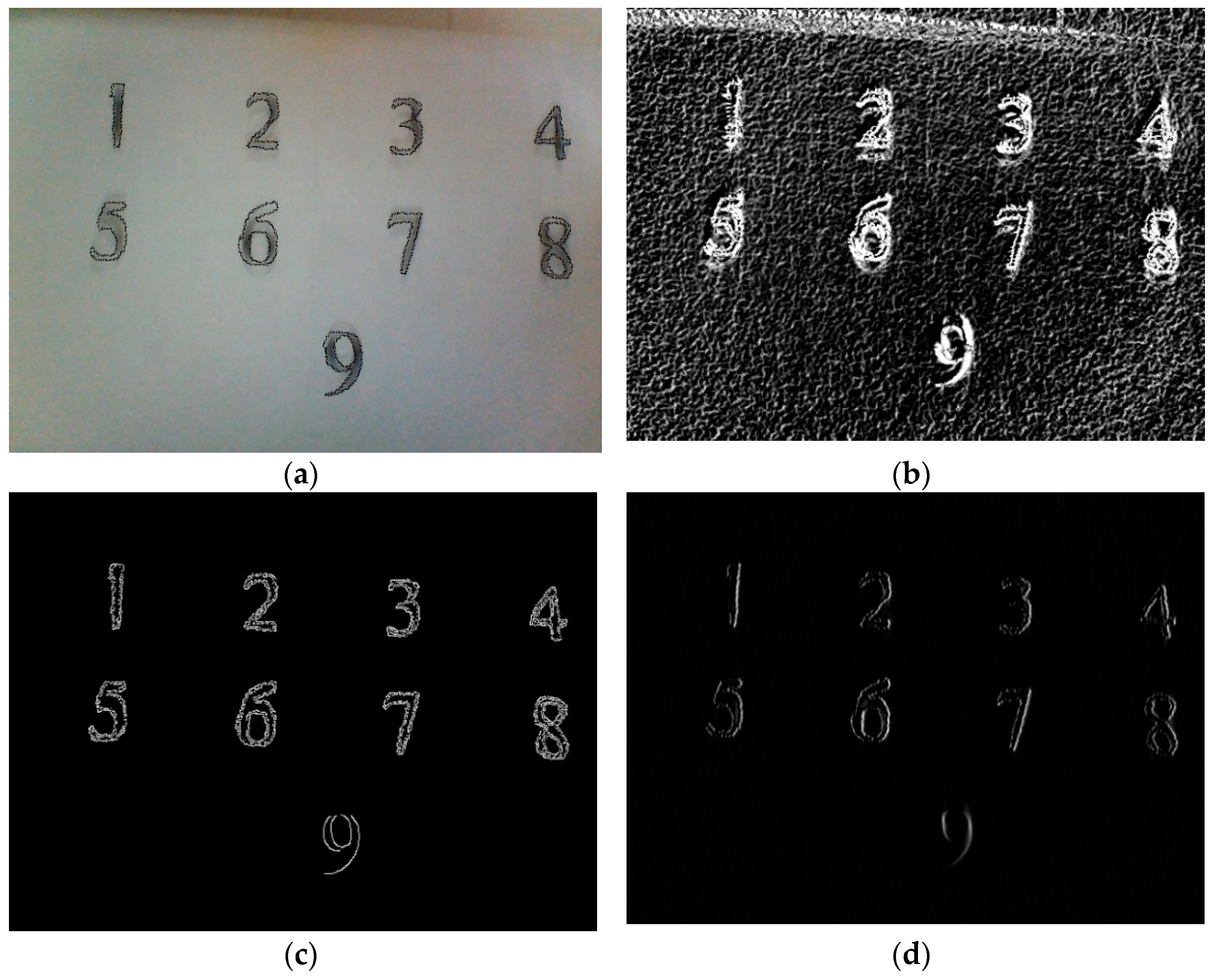
We performed an experiment in which the edges of the source objects were marked on the input image in one of the raster graphics editors. Figure 31a shows the image taken at 50 lux, Figure 31b shows the filtered image of the Sobel operator, Figure 31c shows the Canny operator, and Figure 31d shows Prewitt’s operator. As a result of filtering, more edges from the original image were formed in Prewitt and Canny, which is seen subjectively. An experiment was performed to compare the input image with the filtered images using PSNR, and the results are shown:
Input image, img_sobel—11.7;
Input image, img_canny—13.76;
Input image, img_prewitt’s—14.67.
This is best performed by Prewitt’s operator, as the PSNR values are the highest.
5. Discussion
The experiments show that to create an adaptive system, you can use the technique of selecting filters, for which you need to choose a filter that provides the best symmetry of the images under appropriate conditions. The success of the experiments inspires the authors to further test all the most widely used filters in different conditions, which will allow (according to an objective assessment) choosing filters that provide the best symmetry of image display for specific conditions.
In image segmentation evaluation, the structural similarity index (SSIM) estimates the visual impact of shifts in an image [26]. The SSIM consists of three local comparison functions, namely luminance comparison, contrast comparison, and structure comparison, between two signals excluding other remaining errors. The SSIM is computed locally by moving an 8 × 8 window for each pixel, unlike the peak signal-to-noise ratio (PSNR) or root-mean-square error (RMSE), which are measured at the global level. “Even though SSIM can be applied in the case of an edge detection evaluation, in the presence of too many areas without contours, the obtained score is not efficient or useful (in order to judge the quality of edge detection with the SSIM, it is necessary to compare with an image having detected edges situated throughout the image areas)” [26]. This is why PSNR was chosen as a simple and widespread method of global assessment. Other popular evaluation methods [26] do not have strong superiority and have less popularity. Due to this, this paper had an unsettled task of studying the behavior of filters in a particular education (without strong differences).
The success of this study encourages the authors to expand the number of methods and conditions in the next study, in particular to conduct experimental studies of additional methods [27]. This paper analyzes the speed in contrast to the idea of lighting level.
6. Conclusions
The conducted experiments show that among the considered methods, in all conditions, only variations of the Sobel operator compete for the title of the best. With different lighting, different variations can be considered the best. In addition, although there is a difference in quality between variations of the Sobel operator, with all types of lighting, they all give a good result. All others highlight the characteristics rather weakly. The resulting dependence presented in the diagram allows fully automating the process of selecting a filter for image preprocessing when designing adaptive computer vision.
Author Contributions
Conceptualization, V.H. and M.M.; methodology, M.M.; software, M.N.; validation, M.N., M.N.; formal analysis, V.H.; investigation, M.M.; resources, M.N.; data curation, M.N.;writing—original draft preparation, V.H.; writing—review and editing, M.N.; visualization, M.N.; supervision, V.H.; project administration, V.H. All authors have read and agreed to the published version of the manuscript.
Funding
This research received no external funding.
Data Availability Statement
Not applicable.
Conflicts of Interest
The authors declare that they have no known competing financial interests or personal relationships that could have appeared to influence the work reported in this paper.
References
- Boyko, I.; Petryk, M.; Fraissard, J. Investigation of the electron-acoustic phonon interaction via the deformation and piezoelectric potentials in AlN/GaN resonant tunneling nanostructures. Superlattices Microstruct. 2021, 156, 106928. [Google Scholar] [CrossRef]
- Petryk, M.R.; Boyko, I.V.; Khimich, O.M.; Petryk, M.M. High-Performance Supercomputer Technologies of Simulation and Identification of Nanoporous Systems with Feedback for n-Component Competitive Adsorption. Cybern. Syst. Anal. 2021, 57, 316–328. [Google Scholar] [CrossRef]
- Boyko, I.; Mudryk, I.; Petryk, M.; Petryk, M. High-Performance Adsorption Modeling Methods with Feedback-Influynces in n-component Nanoporous Media. In Proceedings of the 2021 11th International Conference on Advanced Computer Information Technologies, Deggendorf, Germany, 15–17 September 2021; pp. 441–444. [Google Scholar]
- Mashkov, O.; Krak, Y.; Babichev, S.; Bardachov, Y.; Lytvynenko, V. Preface Lecture Notes on Data Engineering and Communications; Springer: Berlin, Germany, 2022; Volume 77, pp. v–vi. [Google Scholar]
- Hrytsyk, V.; Nazarkevych, M. Real-Time Sensing, Reasoning and Adaptation for Computer Vision Systems. In ISDMCI 2021: Lecture Notes in Computational Intelligence and Decision Making; Springer: Cham, Switzerland, 2021; pp. 573–585. [Google Scholar]
- Hrytsyk, V.; Grondzal, A.; Bilenkyj, A. Augmented reality for people with disabilities. In Proceedings of the 2015 Xth International Scientific and Technical Conference” Computer Sciences and Information Technologies” (CSIT), Lviv, Ukraine, 14–17 September 2015; pp. 188–191. [Google Scholar]
- Beucher, A.; Fröjdö, S.; Österholm, P.; Martinkauppi, A.; Edén, P. Fuzzy Logic for Acid Sulfate SoilMapping: Application to the Southern Part of the Finnish Coastal Areas. Geoderma 2014, 226–227, 21–30. [Google Scholar] [CrossRef]
- Nazarkevych, M.; Hrytsyk, V.; Voznyi, Y.; Marchuk, A.; Vozna, O. Method of detecting special points on biometric images based on new filtering methods. Proc. CEUR Workshop Proc. 2021, 243–251. Available online: http://ceur-ws.org/Vol-2923/paper26.pdf (accessed on 26 March 2022).
- Nazarkevych, M.; Dmytruk, S.; Hrytsyk, V.; Maslanych, I.; Sheketa, V. Evaluation of the effectiveness of different image skeletonization methods in biometric security systems. Int. J. Sens. Wirel. Commun. Control 2021, 11, 542–552. [Google Scholar] [CrossRef]
- Kamińska, D.; Aktas, K.; Rizhinashvili, D.; Moeslund, T.B.; Anbarjafari, G. Two-stage recognition and beyond for compound facial emotion recognition. Electronics 2021, 10, 2847. [Google Scholar] [CrossRef]
- Aakerberg, A.; Nasrollahi, K.; Moeslund, T.B. Real-world super-resolution of face-images from surveillance cameras. IET Image Processingthis 2022, 16, 442–452. [Google Scholar] [CrossRef]
- Nazarkevych, M.; Voznyi, Y.; Hrytsyk, V.; Havrysh, B.; Lotoshynska, N. Identification of biometric images by machine learning. In Proceedings of the 2021 IEEE 12th International Conference on Electronics and Information Technologies (ELIT), Lviv, Ukraine, 19–21 May 2021; pp. 95–98. [Google Scholar]
- Nazarkevych, M.; Lotoshynska, N.; Hrytsyk, V.; Vozna, O.; Palamarchuk, O. Design of biometric system and modeling of machine learning for entering the information system. Int. Sci. Tech. Conf. Comput. Sci. Inf. Technol. 2021, 2, 225–230. [Google Scholar]
- Prandi, C.; Barricelli, B.R.; Mirri, S.; Fogl, D. Accessible wayfinding and navigation: A systematic mapping study. Univers. Access Inf. Soc. 2021, 1–28. [Google Scholar] [CrossRef]
- Duda, O.R.; Hart, E.P. Pattern Classification and Scene Analysis; Wiley: New York, NY, USA, 1973; 482p. [Google Scholar]
- Martin, D.; Fowlkes, C.; Tal, D.; Malik, J. A Database of Human Segmented Natural Images and its Application to Evaluating Segmentation Algorithms and Measuring Ecological Statistics. In Proceedings of the Eighth IEEE International Conference on Computer Vision, ICCV 2001, Vancouver, BC, Canada, 7–14 July 2001; Volume 23. [Google Scholar]
- Canny, J. A computational approach to edge detection. IEEE Trans. Pattern Anal. Mach. Intell. 1986, 8, 679–698. [Google Scholar] [CrossRef]
- Lindeberg, T. Normative theory of visual receptive fields. Heliyon 2021, 7, e05897. [Google Scholar] [CrossRef] [PubMed]
- Jansson, Y.; Lindeberg, T. Dynamic Texture Recognition Using Time-Causal and Time-Recursive Spatio-Temporal Receptive Fields. J. Math. Imaging Vis. 2018, 60, 1369–1398. [Google Scholar] [CrossRef] [Green Version]
- Beucher, A.; Rasmussen, C.B.; Moeslund, T.B.; Greve, M.H. Interpretation of Convolutional Neural Networks for Acid Sulfate Soil Classification. Front. Environ. Sci. 2022, 9, 809995. [Google Scholar] [CrossRef]
- Rasmussen, C.B.; Lejbølle, A.R.; Nasrollahi, K.; Moeslund, T.B. Evaluation of Edge Platforms for Deep Learning in Computer Vision; Lecture Notes in Artificial Intelligence and Lecture Notes in Bioinformatics; LNCS: Berlin, Germany, 2021; Volume 12664, pp. 523–537. [Google Scholar]
- Alarcao, S.M.; Fonseca, M.J. Emotions recognition using EEG signals: A survey. IEEE Trans. Affect. Comput. 2017, 10, 374–393. [Google Scholar] [CrossRef]
- Mamun, I. Image Classification Using SSIM. Towards Data Science. Available online: https://towardsdatascience.com/image-classification-using-ssim-34e549ec6e12 (accessed on 26 March 2022).
- Everts, I.; Van Gemert, J.C.; Gevers, T. Evaluation of color spatio-temporal interest points for human action recognition. IEEE Trans. Image Processing 2014, 23, 1569–1580. [Google Scholar] [CrossRef] [Green Version]
- Spontón, H.; Cardelino, J. A Review of Classic Edge Detectors. Image Processing Line 2015, 5, 90–123. [Google Scholar] [CrossRef] [Green Version]
- Magnier, B. Edge detection: A review of dissimilarity evaluations and a proposed normalized measure: Review. Multimed. Tools Appl. 2018, 77, 9489–9533. [Google Scholar] [CrossRef] [Green Version]
- Tariq, N.; Hamzah, R.A.; Ng, T.F.; Wang, S.L.; Ibrahim, H. Quality Assessment Methods to Evaluate the Performance of Edge Detection Algorithms for Digital Image: A Systematic Literature Review. IEEE Access 2021, 9, 87763–87776. [Google Scholar] [CrossRef]
- Sobel, I.; Feldman, G. A 3 × 3 Isotropic Gradient Operator for Image Processing. Pattern Classif. Scene Anal. 1973, 271–272. [Google Scholar]
- Canny, J.F. Finding Edges and Lines in Images. Master’s Thesis, MIT AI Laboratory, Cambridge, CA, USA, 1983; 720p. [Google Scholar]
- Ding, L.; Goshtasby, A. On the Canny edge detector. Pattern Recognit. 2001, 34, 721–725. [Google Scholar] [CrossRef]
- Prewitt, J.M. Object enhancement and extraction. Pict. Processing Psychopictorics 1970, 10, 15–19. [Google Scholar]
Figure 1.
Gradient direction.

Figure 2.
(a) Input image; (b) Sobel gradient at 70 lux.

Figure 3.
(a) Normalized Sobel gradient of the image along the x-axis; (b) normalized Sobel gradient of the image on the y-axis at 70 lux.
Figure 3.
(a) Normalized Sobel gradient of the image along the x-axis; (b) normalized Sobel gradient of the image on the y-axis at 70 lux.

Figure 4.
(a) Canny’s operator; (b) Prewitt’s operator at 70 lux.

Figure 5.
(a) Prewitt’s operator X; (b) Prewitt’s operator Y at 70 lux.

Figure 6.
(a) Input image; (b) Sobel operator at 50 lux.

Figure 7.
(a) Sobel operator on the x-axis; (b) Sobel operator on the y-axis at 50 lux.

Figure 8.
(a) Canny operator; (b) Prewitt’s operator on the y-axis at 50 lux.

Figure 9.
(a) Prewitt’s operator on the x-axis; (b) Prewitt’s operator on the y-axis at 50 lux.

Figure 10.
(a) Input image; (b) Sobel operator at 100 lux.

Figure 11.
(a) Sobel operator on the x-axis; (b) Sobel operator on the y-axis at 100 lux.

Figure 12.
(a) Canny operator; (b) Prewitt’s operator on the y-axis at 100 lux.

Figure 13.
(a) Prewitt’s operator on the x-axis; (b) Prewitt’s operator on the y-axis at 100 lux.

Figure 14.
(a) Input image; (b) Sobel operator at 260 lux.

Figure 15.
(a) Sobel operator on the x-axis; (b) Sobel operator on the y-axis at 260 lux.

Figure 16.
(a) Canny operator; (b) Prewitt’s operator at 260 lux.

Figure 17.
(a) Prewitt’s operator X; (b) Prewitt’s operator Y at 260 lux.

Figure 18.
(a) Input image; (b) Sobel operator at 2300 lux.

Figure 19.
(a) Sobel operator on the x-axis; (b) Sobel operator on the y-axis at 2300 lux.

Figure 20.
(a) Canny operator; (b) Prewitt’s operator at 2300 lux.

Figure 21.
(a) Prewitt’s operator X; (b) Prewitt’s operator Y at 2300 lux.

Figure 22.
(a) input image; (b) Sobel operator at 2300 lux+ man shadow.

Figure 23.
(a) Sobel operator on the x-axis; (b) Sobel operator on the y-axis at 2300 lux+ man shadow.
Figure 23.
(a) Sobel operator on the x-axis; (b) Sobel operator on the y-axis at 2300 lux+ man shadow.

Figure 24.
(a) Canny operator; (b) Prewitt’s operator at 2300 lux+ man shadow.

Figure 25.
(a) Prewitt’s operator X; (b) Prewitt’s operator y at 2300 lux+ man shadow.

Figure 26.
(a) input image; (b) Sobel operator at 2350 lux.

Figure 27.
(a) Sobel operator on the x-axis; (b) Sobel operator on the y-axis at 2350 lux.

Figure 28.
(a) Canny operator; (b) Prewitt’s operator at 2350 lux.

Figure 29.
(a) Prewitt’s operator X; (b) Prewitt’s operator Y at 2350 lux.

Figure 30.
Results of objective assessment (PSNR) of symmetry of researched operations.

Figure 31.
(a) Input image; (b) Sobel operator; (c) Canny operator; (d) Prewitt’s operator.


Table 1.
Lighting on the object in the Suites.
| Intensity Scale | Lighting on the Object in the Suites | Inside the Near Window, Lux/Time |
|---|---|---|
| 108 | The Sun disc is at noon | |
| 106 | Glitter of water and metal under sunlight | |
| 104 | Snow-covered snow and clouds. Illuminated objects by day | 2300/13:30 260/13:00 |
| 102 | Objects in the shade, in the afternoon | 100/16:50 70/16:00 (the sun came out of the clouds) 50/16:30 |
| 100 | Moon | |
| 10−2 | Stars |
Publisher’s Note: MDPI stays neutral with regard to jurisdictional claims in published maps and institutional affiliations. |
© 2022 by the authors. Licensee MDPI, Basel, Switzerland. This article is an open access article distributed under the terms and conditions of the Creative Commons Attribution (CC BY) license (https://creativecommons.org/licenses/by/4.0/).
Share and Cite
MDPI and ACS Style
Hrytsyk, V.; Medykovskyy, M.; Nazarkevych, M. Estimation of Symmetry in the Recognition System with Adaptive Application of Filters. Symmetry 2022, 14, 903. https://doi.org/10.3390/sym14050903
AMA Style
Hrytsyk V, Medykovskyy M, Nazarkevych M. Estimation of Symmetry in the Recognition System with Adaptive Application of Filters. Symmetry. 2022; 14(5):903. https://doi.org/10.3390/sym14050903
Chicago/Turabian StyleHrytsyk, Volodymyr, Mykola Medykovskyy, and Mariia Nazarkevych. 2022. "Estimation of Symmetry in the Recognition System with Adaptive Application of Filters" Symmetry 14, no. 5: 903. https://doi.org/10.3390/sym14050903
Note that from the first issue of 2016, this journal uses article numbers instead of page numbers. See further details here.