Spare Parts Transportation Optimization Considering Supportability Based on Uncertainty Theory

Abstract

Ensuring a consistent, continuous, and efficient spare parts supply is a critical issue that must be addressed in the equipment support system. In order to effectively improve the coverage level and handle the common asymmetry information present in practical applications, the spare parts transport vehicle routing and scheduling model was further optimized. We integrated supportability requirements and uncertainty theory into the model to better describe the actual uncertain demand of each site. We selected three critical supportability indicators as constraints, redefined them with uncertain variables, and then completed the chance-constrained model on this basis. Once the confidence level is specified, the uncertain constraints can be transformed into deterministic constraints, and finally, the equivalent deterministic model can be solved easily. In addition, a feasible solution can be found through a genetic algorithm, and a numerical example is provided to validate the model’s rationality. The proposed method successfully seeks the balance between the total cost and supportability.

1. Introduction

The equipment support system refers to the organic combination of all support resources and management required by the equipment during the operation and support phases. It can meet the requirements of operational readiness and sustainability by interconnecting and coordinating the resources required. The design of the support system is critical because the final efficiency of the support system affects the smooth realization of equipment functions. With the development of science and technology, equipment complexity and maintenance difficulty increase, and support issues become more prominent. As a result, it is becoming increasingly important to develop a scientific and efficient support system to maintain, restore, and improve the overall performance of the material system.

Support resources are the foundation of the equipment support system. The ability to support spare parts has a direct impact on the reliability, availability, and maintenance of the material system. Therefore, ensuring a consistent, continuous, and efficient spare parts supply is essential. In order to guarantee the spare parts supply, Wong et al. proposed a double-layer and multi-variety spare parts inventory optimization method under the background of allowing parallel supply in emergencies [1]. Holmström et al. integrated rapid manufacturing into the spare parts supply system [2]. Liu et al. proved that layered manufacturing technology could effectively increase the capacity of spare parts supply and reduce total cost [3]. These methods included storing more spare parts at each site to prevent demand fluctuations or storing fewer or no spare parts at each site until a shortage occurs, then delivering. However, these methods paid little attention to the optimal choice of transportation routes. In reality, due to the supply system’s limited transportation capacity, reasonable transportation routes must be planned in order for spare parts to be delivered to the site in demand on time. At present, the multi-level support system is common and practical. In this case, optimizing the spare parts transportation strategy across all levels of sites could effectively reduce spare parts shortages and improve spare parts supply capacity. In this way, it is possible to avoid the situation where the equipment is in maintenance or waiting for support for too long. Finally, the purpose of accurate support is achieved.

Recently, in the study of supply networks, researchers chose many different factors as constraints of the vehicle routing planning model for various reasons [4,5]. Ettl et al. took lead time, demand, service level, and other factors into consideration when establishing the optimization model [6]. Edyta Kucharska took into account various elements causing dynamism [7]. Touboulic et al. discussed how participatory research supports the development of supply chain management (SCM) theory and practice [8]. Gayialis et al. considered various parameters and restrictions such as traffic congestion, working hours, and state regulations in a holistic way when designing an innovative vehicle routing and scheduling system in an urban environment [9]. However, solutions to these vehicle routing problems are not entirely suitable for spare parts transportation. They did not consider the vehicle routing planning model from the perspective of supportability, which led to the neglect of the losses caused by the untimely spare parts supply. Furthermore, each site’s supply priority varies due to the different rates of spare parts loss. If these factors are not considered when transporting spare parts, equipment downtime may be prolonged. In the end, it results in more losses.

To summarize, we discovered two problems. First, spare parts supply pays little attention to optimizing transportation routes. Second, the existing transportation route optimization methods are seldom considered from the standpoint of supportability.

Croston emphasized the importance of demand forecasting in 1972 and put forward many models for spare parts demand estimation and forecasting [10,11,12]. In the process of further research, we found that many researchers use probability theory to predict supply through historical data. According to different supply backgrounds, the probability distribution varies. Liu et al. studied the three-level supply structure model of repairable spare parts in wartime and gave the spare parts supply formula under Poisson distribution [13]. Ronzoni et al. put forward the spare parts management method using probabilistic dynamic programming, assuming that spare parts demand obeys Bernoulli distribution [14]. Methods for constructing confidence intervals for the extreme values of any continuous distribution were developed [15]. Therefore, data analysis inaccuracies caused by outliers can be efficiently avoided. The continuous distribution, such as truncated normal distributions and Weibull distributions, can also be used to fit the data [16,17,18,19,20]. When considering the long-term supply situation, a stochastic process is also a solution [1]. In addition to determining the demand based on classic random distribution or random process, simulation or artificial intelligence methods are also used to predict the spare parts demand in the case of a large amount of historical data [21,22].

However, we have two questions: Can we collect enough historical data? Can we believe that the distribution fitted by historical data is close to the actual distribution?

The new equipment has a technological leap-forward update as a result of technological innovation. However, because historical spare parts consumption data are scarce, it is difficult to grasp the statistical law that influences spare parts supply. Considering that there are many uncertain factors affecting the spare parts demand, and the current understanding level is limited, it is not easy to understand the demand from probability [23]. Moreover, because of the limitation of the Law of Large Numbers, we have reservations about applying probability theory to deal with uncertain demands. In view of this problem, some researchers have put forward a simulation method based on empirical data and traditional prediction models [23,24]. Thus, we believe that the uncertain spare parts demand can also be described by collecting empirical data. For example, after the new equipment is put into production, we can learn about the information of spare parts by asking experts. However, the difference in experience between expert A and expert B makes them give different consumption estimated amounts [25,26]. Therefore, developing an optimization model that takes into account the existing uncertainty caused by human cognition is a pressing issue.

Liu first formulated a project-scheduling problem where the duration times were expressed as uncertain variables [27]. Subsequently, many uncertain programming models were studied to handle project-scheduling problems under an uncertain environment. Furthermore, Zhou et al. defined the route optimality constraints of uncertain expected minimum spanning tree (MST) and uncertain α-MST [28]. Recently, Majumder et al. proposed a multi-objective minimum spanning tree problem (MMSTP) with indeterminate problem parameters and successfully applied it to optimize the distribution of petroleum products [29]. According to these studies, we believe that uncertainty theory can effectively describe the uncertainty in demand and successfully solve the route optimality problem under an uncertain environment.

This article intends to establish a vehicle routing optimality model in the background of comprehensive support applications, with the goal of lowering total cost while improving system support capability. Simultaneously, uncertainty theory is introduced to address the constraints of missing historical spare parts consumption data. The structure of this paper is as follows: in the second section, some definitions and theorems of uncertainty theory are introduced, which provides a mathematical basis for the establishment of the model. In section three, we describe the problem, explain the hypothesis and representation method of the model, and further give the spare parts transportation optimization method based on an uncertain chance-constrained model. The fourth section gives the concrete steps of solving the model through a genetic algorithm. Finally, an example is given to verify the operability of the model and algorithm.

2. Preliminaries on Uncertainty Theory

In the current practical engineering applications, the historical data of many new spare parts are missing. Therefore, it is necessary to rely on expert experience data to evaluate the relevant spare parts information. However, when experts provide empirical data, subjective judgments and asymmetry information exist. In other words, the data are heavily influenced by the individual’s cognitive level. Thus, during analysis, epistemic uncertainty should not be ignored; otherwise, it may lead to inaccuracy or underestimation of the supportability indicators of spare parts. In order to analyze this uncertain phenomenon better, we take uncertainty theory as a choice.

The uncertainty theory was founded by Liu in 2007 and subsequently studied by many researchers [30,31]. This section mainly introduces some basic definitions and theorems of uncertainty theory to provide a theoretical basis for the optimization model of spare parts transportation under uncertain demand.

The uncertain measure is a set function that satisfies the axioms of uncertainty theory. Γ is a nonempty set (sometimes called a universal set) and $ℒ$ is a σ-algebra over Γ. Each element Λ in $ℒ$ is called a measurable set, and the uncertain measure $ℳ$ is defined on the σ-algebra $ℒ$. That is, a number $ℳ\left\{\mathsf{\Lambda }\right\}$ is assigned to each event Λ to indicate the belief degree with which we believe Λ will happen [30].

Axiom 1.

(Normality Axiom [30]) $ℳ\left\{\mathsf{\Gamma }\right\}=1$ for the universal set Γ.

Axiom 2.

(Duality Axiom [30]) $ℳ\left\{\mathsf{\Lambda }\right\}+ℳ\left\{{\mathsf{\Lambda }}^{\mathrm{c}}\right\}=1$ for any event Λ.

Axiom 3.

(Subadditivity Axiom [30]) For every countable sequence of events ${\mathsf{\Lambda }}_1,{\mathsf{\Lambda }}_2,\dots ,$ we have

$$ℳ\left\{{\displaystyle \underset{i=1}{\overset{\infty }{\cup }}{\Lambda }_i}\right\}\le {\displaystyle \sum _{i=1}^{\infty }ℳ\left\{{\Lambda }_i\right\}}.$$

(1)

Definition 1.

(Uncertain Measure [30]) The set function $ℳ$ is called an uncertain measure if it satisfies the normality, duality, and subadditivity axioms.

Axiom 4.

(Product Axiom [32]) Let (Γ_k, $ℒ$_k, $ℳ$_k) be uncertainty spaces for k = 1, 2,…The product uncertain measure M is an uncertain measure satisfying

$$ℳ\left\{{\displaystyle \prod }_{\mathrm{k}=1}^{\infty }{\mathsf{\Lambda }}_k\right\}=\underset{k=1}{\overset{\infty }{{\displaystyle \Lambda }}}{ℳ}_k\left\{{\mathsf{\Lambda }}_k\right\}$$

(2)

where Λ_k are arbitrarily chosen events from L_k for k = 1, 2,…, respectively.

The uncertain variable is used to represent quantities with uncertainty.

Definition 2.

(Uncertain Variable [30]) An uncertain variable is a function ξ from an uncertainty space (Γ,$ℒ$,$ℳ$) to the set of real numbers such that $\left\{\xi \in B\right\}$ is an event for any Borel set B of real numbers.

Definition 3.

(Uncertainty Distribution [30]) The uncertainty distribution Φ of an uncertain variable ξ is defined by

$$\Phi \left(x\right)=ℳ\left\{\xi \le x\right\}$$

(3)

for any real number x.

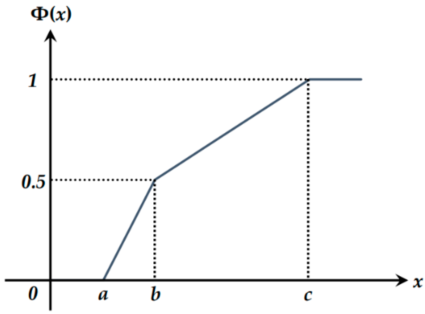
Definition 4.

(Zigzag Uncertainty Distribution [27]) An uncertain variable ξ is called zigzag if it has a zigzag uncertainty distribution

$$\Phi \left(x\right)=\{\begin{array}{ll}0,\hfill & if x\le a\hfill \\ \frac{x-a}{2\left(b-a\right)},\hfill & if a\le x\le b\hfill \\ \frac{\left(x+c-2b\right)}{2\left(c-b\right)},\hfill & if b\le x\le c\hfill \\ 1,\hfill & if x\ge c\hfill \end{array}$$

(4)

denoted byƵ(a,b,c) where a, b, c are real numbers with a < b < c. See Figure 1.

Theorem 1.

(Measure Inversion Theorem [27]) Let ξ be an uncertain variable with uncertainty distribution Φ. Then for any real number x, we have

$$ℳ\left\{\xi \le x\right\}=\Phi \left(x\right), ℳ\left\{\xi >x\right\}=1-\Phi \left(x\right).$$

(5)

Definition 5.

(Regular Uncertainty Distribution [27]) An uncertainty distribution Φ(x) is said to be regular if it is a continuous and strictly increasing function with respect to x at which 0 < Φ(x) < 1, and

$$\underset{x\to -\infty }{\lim }\Phi \left(x\right)=0, \underset{x\to +\infty }{\lim }\Phi \left(x\right)=1.$$

(6)

Definition 6.

(Inverse Uncertainty Distribution [27]) Let ξ be an uncertain variable with regular uncertainty distribution Φ(x). Then the inverse function ${\Phi }^{-1}\left(\alpha \right)$ is called the inverse uncertainty distribution of ξ.

Theorem 2.

(Liu [33]) Let ξ be an uncertain variable with inverse uncertainty distribution ${\Phi }^{-1}\left(\mathsf{\alpha }\right)$.

Then

$$ℳ\left\{\xi \le c\right\}\ge \alpha$$

(7)

if and only if

$${\Phi }^{-1}\left(\alpha \right)\le c$$

(8)

where α and c are constants with 0 < α < 1.

Theorem 3.

(Liu [33]) A function ${\Phi }^{-1}:\left(0,1\right)\to \Re$ is the inverse uncertainty distribution of an uncertain variable ξ if and only if it is continuous and

$$ℳ\left\{\xi <{\Phi }^{-1}\left(\alpha \right)\right\}=\alpha$$

(9)

for all$\alpha \in \left(0,1\right)$.

Theorem 4.

(Sufficient and Necessary Condition [34]) A function ${\Phi }^{-1}:\left(0,1\right)\to \Re$ is an inverse uncertainty distribution if and only if it is a continuous and strictly increasing function.

The independence of two uncertain variables means that knowing the value of one does not change our estimation of the value of the other [33].

Definition 7.

(Independence [32]) The uncertain variables ${\xi }_1,{\xi }_2,\dots ,{\xi }_n$ are said to be independent if

$$ℳ\left\{{\displaystyle \bigcap }_{i=1}^n\left({\xi }_i\in B_i\right)\right\}=\underset{i=1}{\overset{n}{{\displaystyle \Lambda }}}ℳ\left\{\left({\xi }_i\in B_i\right)\right\}$$

(10)

for any Borel sets $B_1,B_2,\dots ,B_n$ of real numbers.

Theorem 5.

(Liu [33]) Let ${\xi }_1,{\xi }_2,\dots ,{\xi }_n$ be independent uncertain variables, and let f₁,f₂,…,f_n be measurable functions. Then $f_1\left({\xi }_1\right),f_2\left({\xi }_2\right),\dots ,f_n\left({\xi }_n\right)$ are independent uncertain variables.

Theorem 6.

(Operational Law [27]) Let ${\xi }_1,{\xi }_2,\dots ,{\xi }_n$ be independent uncertain variables with regular uncertainty distributions${\Phi }_1,{\Phi }_2,\dots ,{\Phi }_n$, respectively. If$f\left(x_1,x_2,\dots ,x_n\right)$ is continuous, strictly increasing with respect to$x_1,x_2,\dots ,x_m$ and strictly decreasing with respect to$x_{m+1},x_{m+2},\dots ,x_n$, then

$$\xi =f\left({\xi }_1,{\xi }_2,\dots ,{\xi }_n\right)$$

(11)

has an inverse uncertainty distribution

$${\Psi }^{-1}\left(\alpha \right)=f\left({\Phi }_1^{-1}\left(\alpha \right),\dots ,{\Phi }_m^{-1}\left(\alpha \right),{\Phi }_{m+1}^{-1}\left(1-\alpha \right),\dots ,{\Phi }_n^{-1}\left(1-\alpha \right)\right).$$

(12)

3. Uncertain Chance-Constrained Model of Spare Parts Transportation

The role of a spare parts warehouse is to provide new spare parts for its surrounding sites in demand to ensure their reliable operation. We assume that there are multiple vehicles available for transportation. Because of the restrictions on transportation capacity and cost, choosing a good transportation strategy is critical to improving the support system’s efficiency. In order to reach the goal of improving the supply capability, a transportation optimization model should be established that can strike a balance between satisfying supportability requirements and lowering total costs. Given the low replacement rate of some new spare parts, there are few or no samples of historical data on their reliability. At the same time, the spare parts demand at each site is uncertain due to the different working environments of the equipment at each site. In this case, the information received by the spare parts warehouse is asymmetrical. Therefore, we choose to use uncertainty theory to infer the spare parts demand from expert belief degree data.

The chance-constrained models can be used to deal with programming problems with uncertain variables. Because of the uncertainty, constraints are frequently not expressed by a specific formula, and it is impossible to guarantee that the constraints can be met before the uncertainty variables are observed. The principle of confidence level is put forward at this point: to some extent, the decision is allowed to fail to meet the constraint conditions, but the constraints must be established above a certain confidence level. In solving the chance-constrained programming, once the confidence level is given in advance, the uncertain constraints can be transformed into deterministic constraints, respectively, and finally, the equivalent deterministic model can be solved.

3.1. Model Assumption

We made the following assumptions:

• The equipment supply network consists of a spare parts warehouse and multiple sites, and only one kind of spare parts is transported;
• The spare parts demand of each site is an uncertain variable, and the site’s demand is independent of each other;
• The transportation paths of spare parts storage and maintenance sites are all connected. The transportation cost is only related to the distance between sites;
• The importance level of each site is the same;
• All transport vehicles are the same, and each vehicle can transport spare parts to any site.

3.2. Symbol Description

Some symbols are used in the model, and they are described in

Table 1. Parameter description table.

Symbol	Description
n	total number of work sites
$i,j$	$\mathrm{index} \mathrm{of} \mathrm{work} \mathrm{sites}, i,j=1,2,\dots ,n$$, i=0$ means warehouse
m	total number of transport vehicles
k	$\mathrm{index} \mathrm{of} \mathrm{transport} \mathrm{vehicles}, k=1,2,\dots ,m$
$d\left(i,j\right)$	$\mathrm{the} \mathrm{distance} \mathrm{between} \mathrm{site} i \mathrm{and} j, i,j=1,2,\dots ,n$
${\xi }_i$	$\mathrm{the} \mathrm{uncertain} \mathrm{spare} \mathrm{parts} \mathrm{demand} \mathrm{of} \mathrm{site} i, i=1,2,\dots ,n$
${\Phi }_i\left(x\right)$	$\mathrm{the} \mathrm{uncertainty} \mathrm{distribution} \mathrm{of} {\xi }_i$$, i=1,2,\dots ,n$
${\Phi }_i^{-1}\left(x\right)$	$\mathrm{the} \mathrm{inverse} \mathrm{uncertainty} \mathrm{distribution} \mathrm{of} {\xi }_i$$, i=1,2,\dots ,n$
$N_i$	$\mathrm{number} \mathrm{of} \mathrm{equipment} \mathrm{at} \mathrm{site} i, i=1,2,\dots ,n$
Z	number of spare parts installed per equipment
$c_1$	transportation cost per unit distance
$c_2$	ordering cost of a single spare part
$R_i$	$\mathrm{the} \mathrm{distance} \mathrm{between} \mathrm{site} i \mathrm{and} \mathrm{warehouse}, i=1,2,\dots ,n$
$A_i$	$\mathrm{the} \mathrm{lower} \mathrm{limit} \mathrm{of} \mathrm{supply} \mathrm{availability} \mathrm{for} \mathrm{site} i, i=1,2,\dots ,n$
$D_i$	$\mathrm{the} \mathrm{maximum} \mathrm{supply} \mathrm{delay} \mathrm{time} \mathrm{for} \mathrm{site} i, i=1,2,\dots ,n$
$A_0$	the lower limit of system availability
l	penalty coefficient
V	the average speed of transport vehicles per unit distance

ξ_i ($i=1,2,\dots ,n$) is an uncertain variable with zigzag uncertainty distribution Φ_i(x), which is denoted by $Z\left(a_i,b_i,c_i\right)$, $a_i<b_i<c_i$.

and

Table 2. Variable description table.

Symbol	Description
$x_{ijk}$	$\mathrm{indicator} \mathrm{variable} x_{ijk}=\{\begin{array}{l}1 \mathrm{vehicle} k \mathrm{transport} \mathrm{from} \mathrm{site} i \mathrm{to} j\\ 0 \mathrm{else}\end{array}$
$z_{ik}$	$\mathrm{indicator} \mathrm{variable} z_{ik}=\{\begin{array}{l}1 \mathrm{vehicle} k \mathrm{deliver} \mathrm{spare} \mathrm{parts} \mathrm{for} \mathrm{site} i\\ 0 \mathrm{else}\end{array}$
$y_i$	$\mathrm{spare} \mathrm{parts} \mathrm{supply} \mathrm{for} \mathrm{site} i, i=1,2,\dots ,n$

.

3.3. Constraint Functions

Supportability refers to the ability of the equipment’s logistics support, supplies, and services to meet the requirements of its normal operation in the ready working states. Supportability, as an integral performance parameter of any integrated system, influences the final performance of the equipment [35,36]. Therefore, designing for supportability is critical in engineering applications. From many optional supportability indicators, we screened out three indicators as constraints of the model, which are the support rate of spare parts, delay time, and supply availability [37]. In order to achieve the overall optimization goal, we must also meet other vehicle transport requirements. In order to satisfy the constraints, all indicators’ confidence levels should be greater than or equal to the values specified. The constraints are outlined below.

3.3.1. Support Rate of Spare Parts Constraint

The support rate of spare parts refers to the proportion that the existing spare parts can meet demand within a specified period. In short, it is the possibility that spare parts are sufficient when spare parts are needed. To avoid a spare part shortage, the support rate of spare parts should be greater than or equal to ${\alpha }_i$:

$$ℳ\left\{{\xi }_i\le y_i\right\}\ge {\alpha }_i,i=1,2,\dots ,n$$

(13)

where ${\xi }_i$ has regular uncertainty distribution ${\Phi }_i\left(x\right)$ and inverse uncertainty distribution ${\Phi }_i^{-1}\left(x\right)$.

3.3.2. Delay Time Constraint

Supply response time refers to the time between receiving a request from the site and the site receiving spare parts, which is mainly related to the distance of delivery. Then the supply response time of the site is T_i:

$$T_i={\displaystyle \sum _{k=1}^m{z}_{ik}}{\displaystyle \sum _{j=1}^i{\displaystyle \sum _{l=0}^n\frac{x_{ljk}d\left(l,j\right)}{V}}}.$$

(14)

The delay time refers to the time spent due to a lack of spare parts related to support rate and supply response time. Thus, the delay time of site i is:

$$T_i^{delay}=\left(1-ℳ\left\{{\xi }_i\le y_i\right\}\right){\displaystyle \sum _{k=1}^m{z}_{ik}}{\displaystyle \sum _{j=1}^i{\displaystyle \sum _{l=0}^n\frac{x_{ljk}d\left(l,j\right)}{V}}}.$$

(15)

The constraint that the delay time of site i should not exceed D_i is:

$$\left(1-ℳ\left\{{\xi }_i\le y_i\right\}\right){\displaystyle \sum _{k=1}^m{z}_{ik}}{\displaystyle \sum _{j=1}^i{\displaystyle \sum _{l=0}^n\frac{x_{ljk}d\left(l,j\right)}{V}}}\le D_i,i=1,2,\dots ,n.$$

(16)

3.3.3. Supply Availability Constraint

Supply availability can be used to measure the impact of spare parts shortage on the use of equipment. In practical applications, it is the ratio of equipment not shut down due to any spare parts shortage to the total amount of equipment [37]. The system requires that the availability of the site i is not less than $A_i$. One of the chance constraints for supply availability is the uncertain measure of the availability of the site i, which is satisfied at $A_i$ should be greater than or equal to:

$$ℳ\left\{{\left[1-({\xi }_i-y_i)\frac{1}{N_{i}Z}\right]}^Z\ge A_i\right\}\ge {\beta }_i,i=1,2,\dots ,n.$$

(17)

A further requirement is the uncertain measure of the availability of a support system which is satisfied at $A_0$ should be greater than or equal to γ:

$$ℳ\left\{{\displaystyle \sum _{i=1}^n{N}_i}{\left[1-({\xi }_i-y_i)\frac{1}{N_{i}Z}\right]}^Z/{\displaystyle \sum _{i=1}^n{N}_i}\ge A_0\right\}\ge \gamma ,i=1,2,\dots ,n.$$

(18)

3.3.4. Vehicle Transport Constraint

There is a total of k spare parts vehicles, which start from the spare parts warehouse and deliver spare parts to each site in demand. At most, one vehicle is required to deliver spare parts for the site i:

$$\sum _{k=1}^m{z}_{ik}\le 1,i=1,2,\dots ,n$$

(19)

There is at most one transport vehicle leaving the site i:

$$z_{ik}\le {\displaystyle \sum _{j=0}^n{x}_{ijk}},i=1,2,\dots ,n,k=1,2,\dots ,m.$$

(20)

There is at most one transport vehicle arriving at the site j:

$$z_{jk}\le {\displaystyle \sum _{i=0}^n{x}_{ijk}},j=1,2,\dots ,n,k=1,2,\dots ,m.$$

(21)

3.4. Objective Function

The objective function of the optimization model mainly considers transportation cost and spare parts ordering cost.

The transportation cost is related to the transport distance and the spare parts support rate of each site to the power of l. Here, l is used as a penalty coefficient. The penalty coefficient represents the loss caused by insufficient supply under different situations. In brief, the transportation cost from site i to site j positively correlates with the distance between them and is related to the spare parts support rate of site i. Therefore, the cost of transporting spare parts from site i to site j is:

$$C_1={\displaystyle \sum _{i=0}^n\frac{{\displaystyle \sum _{j=0}^n{\displaystyle \sum _{k=1}^m{c}_1{x}_{ijk}d\left(i,j\right)}}}{{[1-ℳ\left\{{\xi }_i\le y_i\right\}]}^l}}.$$

(22)

The spare parts ordering costs are only related to the spare parts supply quantity of the site:

$$C_2=c_2\sum _{i=0}^n{y}_i$$

(23)

We can finally obtain the objective function, which is the sum of the overhead costs:

$$C_0=C_1+C_2.$$

(24)

Then, we can obtain the goal of the model shown as follows, which is to minimize the total cost of transporting spare parts:

$$Min{\displaystyle \sum _{i=0}^n\frac{{\displaystyle \sum _{j=0}^n{\displaystyle \sum _{k=1}^m{c}_1{x}_{ijk}d\left(i,j\right)}}}{{[1-ℳ\left\{{\xi }_i\le y_i\right\}]}^l}}+c_2{\displaystyle \sum _{i=0}^n{y}_i}.$$

(25)

In summary, an optimization model of uncertain chance-constrained for multi-vehicle spare parts transportation path optimization is established, as shown below:

$$\{\begin{array}{l}Min{\displaystyle \sum _{i=0}^n\frac{{\displaystyle \sum _{j=0}^n{\displaystyle \sum _{k=1}^m{c}_1{x}_{ijk}d\left(i,j\right)}}}{{[1-ℳ\left\{{\xi }_i\le y_i\right\}]}^l}}+c_2{\displaystyle \sum _{i=0}^n{y}_i}\hfill \\ s.t. \hfill \\ ℳ\left\{{\xi }_i\le y_i\right\}\ge {\alpha }_i,i=1,2,\dots ,n\hfill \\ \left(1-ℳ\left\{{\xi }_i\le y_i\right\}\right){\displaystyle \sum _{k=1}^m{z}_{ik}}{\displaystyle \sum _{j=1}^i{\displaystyle \sum _{l=0}^n\frac{x_{ljk}d\left(l,j\right)}{V}}}\le D_i,i=1,2,\dots ,n\hfill \\ ℳ\left\{{\left[1-\frac{{\xi }_i-y_i}{N_{i}Z}\right]}^Z\ge A_i\right\}\ge {\beta }_i,i=1,2,\dots ,n\hfill \\ ℳ\left\{{\displaystyle \sum _{i=1}^n{N}_i}{\left[1-\frac{{\xi }_i-y_i}{N_{i}Z}\right]}^Z/{\displaystyle \sum _{i=1}^n{N}_i}\ge A_0\right\}\ge \gamma \hfill \\ {\displaystyle \sum _{k=1}^m{z}_{ik}}\le 1,i=1,2,\dots ,n\hfill \\ z_{ik}\le {\displaystyle \sum _{j=0}^n{x}_{ijk}},i=1,2,\dots ,n,k=1,2,\dots ,m\hfill \\ z_{jk}\le {\displaystyle \sum _{i=0}^n{x}_{ijk}},j=1,2,\dots ,n,k=1,2,\dots ,m\hfill \\ x_{ijk}\in \left\{0,1\right\}\hfill \\ z_{ik}\in \left\{0,1\right\}.\hfill \end{array}$$

(26)

When the confidence level is specified, the uncertain chance-constrained condition can be transformed into a deterministic problem for solving. The justification of the deterministic counterpart of the model is depicted here.

Since ξ_i ($i=1,2,\dots ,n$) is an uncertain variable with regular uncertainty distribution Φ_i(x) in Model (26), therefore, the equation $ℳ\left\{{\xi }_i\le y_i\right\}={\Phi }_i\left(y_i\right)$ follows from the definition of uncertainty distribution immediately. Subsequently, the second constraint in Model (26)

$$\left(1-ℳ\left\{{\xi }_i\le y_i\right\}\right){\displaystyle \sum _{k=1}^m{z}_{ik}}{\displaystyle \sum _{j=1}^i{\displaystyle \sum _{l=0}^n\frac{x_{ljk}d\left(l,j\right)}{V}}}\le D_i$$

can be correspondingly expressed as

$$1-{\mathsf{\Phi }}_i\left(y_i\right){\displaystyle \sum _{k=1}^m{z}_{ik}}{\displaystyle \sum _{j=1}^i{\displaystyle \sum _{l=0}^n\frac{x_{ljk}d\left(l,j\right)}{V}}}\le D_i.$$

Following the definition of inverse uncertainty distribution, we obtain that the inverse uncertainty distribution of ξ_i is ${\Phi }_i^{-1}\left(\alpha \right)$. It follows from $ℳ\left\{{\xi }_i\le y_i\right\}={\Phi }_i\left(y_i\right)$ that $ℳ\left\{{\xi }_i\le y_i\right\}\ge {\alpha }_i$ if and only if ${\Phi }_i\left(y_i\right)\ge {\alpha }_i$, i.e., ${\Phi }^{-1}\left({\alpha }_i\right)\le y_i$. The corresponding expression of the first constraint in Model (26) is thus obtained. According to the basic properties of inequalities, it suffices to prove the equation

$$ℳ\left\{{\left[1-\frac{{\xi }_i-y_i}{N_{i}Z}\right]}^Z\ge A_i\right\}\ge {\beta }_i$$

is equivalent to the equation

$$ℳ\left\{{\xi }_i\le \left[\left(1-A_i^{1/Z}\right)\cdot N_{i}Z+y_i\right]\right\}\ge {\beta }_i.$$

An argument similar to the one used in the proof of the first constraint shows that

$${\Phi }_i{}^{-1}\left({\beta }_i\right)\le \left(1-A_i^{1/Z}\right)\cdot N_{i}Z+y_i,i=1,2,\dots ,n.$$

The corresponding expression of the third constraint in Model (26) can be finally obtained. The remainder of the argument is analogous to that mentioned above and is left to the reader. Consequently, Model (27) becomes the crisp equivalent of the Model (26).

$$\{\begin{array}{l}Min{\displaystyle \sum _{i=0}^n\frac{{\displaystyle \sum _{j=0}^n{\displaystyle \sum _{k=1}^m{c}_1{x}_{ijk}d\left(i,j\right)}}}{{[1-{\Phi }_i\left(y_i\right)]}^l}}+c_2{\displaystyle \sum _{i=0}^n{y}_i}\hfill \\ s.t.\hfill \\ {\Phi }_i{}^{-1}\left({\alpha }_i\right)\le y_i,i=1,2,\dots ,n\hfill \\ \left(1-{\Phi }_i\left(y_i\right)\right){\displaystyle \sum _{k=1}^m{z}_{ik}}{\displaystyle \sum _{j=1}^i{\displaystyle \sum _{l=0}^n\frac{x_{ljk}d\left(l,j\right)}{V}}}\le D_i,i=1,2,\dots ,n\hfill \\ {\Phi }_i{}^{-1}\left({\beta }_i\right)-\left(1-A_i^{1/Z}\right)\cdot N_{i}Z\le y_i,i=1,2,\dots ,n\hfill \\ {\displaystyle \sum _{i=1}^n{N}_i}{\left[1-({\Phi }_i^{-1}\left(\gamma \right)-y_i)\frac{1}{N_{i}Z}\right]}^Z/{\displaystyle \sum _{i=1}^n{N}_i}\ge A_0\hfill \\ {\displaystyle \sum _{k=1}^m{z}_{ik}}\le 1,i=1,2,\dots ,n\hfill \\ z_{ik}\le {\displaystyle \sum _{j=0}^n{x}_{ijk}},i=1,2,\dots ,n,k=1,2,\dots ,m\hfill \\ z_{jk}\le {\displaystyle \sum _{i=0}^n{x}_{ijk}},j=1,2,\dots ,n,k=1,2,\dots ,m\hfill \\ x_{ijk}\in \left\{0,1\right\}\hfill \\ z_{ik}\in \left\{0,1\right\}.\hfill \end{array}$$

(27)

4. Genetic Algorithm

In the previous section, the uncertain chance-constrained model was successfully converted to the equivalent deterministic constraint model. The genetic algorithm is used in this section to find the feasible solution for the minimum objective function value.

A genetic algorithm is a classic algorithm for solving VRP problems, and its stability and usability were extensively demonstrated [38]. Since the development of the genetic algorithm, its theoretical system has matured significantly. In order to avoid deviations in the calculation algorithm and results, this article chooses to use this classical genetic algorithm to solve the problem. The optimization process of genetic algorithms is very similar to that of path optimization, so the application of the genetic algorithm in path optimization is relatively standardized. The basic principle of the algorithm is to perform an iterative search for possible solutions. Initialization, fitness evaluation, selection, crossover, and mutation are the general procedures of the genetic algorithm [39,40].

4.1. Initialization Operation

Because the vehicle routing problem is essentially a combinatorial optimization problem, the chromosomes can be encoded as integers. However, in this study, demand can be considered as a continuous parameter that must be encoded as real numbers, which can considerably improve the operation’s accuracy. When generating chromosomes, the structures can be divided into three parts: site, vehicle, and supply, each with its own encoding method. Following that, the various sections of the chromosome are operated separately during selection, crossover, and mutation operations.

4.2. Fitness Function

The fitness function is a function that describes the correspondence between an individual and their fitness. From the objective value of the model, it seeks for minimum, so $\frac{1}{object value}$ is defined as the fitness function.

4.3. Selection Operation

The aim of the selection operation is to select better chromosomes to be the parent. The idea is to give preference to individuals with high fitness scores and allow them to pass their genes to successive generations. This paper adopted the roulette wheel selection method for the selection operation. The scale on the roulette wheel is not average since it is divided according to the fitness of each chromosome. The larger the chromosome’s region on the roulette wheel is, the more probable it is to be chosen.

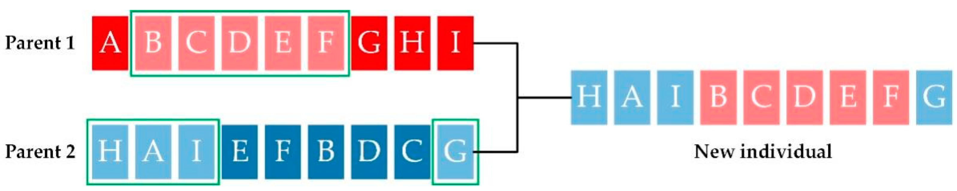
4.4. Crossover Operation

The crossover operation represents mating between individuals. Two individuals are selected as parent chromosomes according to the selection operator, and crossover sites are chosen at random. The genes at these crossover sites are then exchanged, thus creating a completely new individual. The parent chromosome mainly passes on its good traits to the next generation. If a chromosome uses two coding methods at the same time, the crossover can only be operated between the same coding segments. See Figure 2 for an example.

4.5. Mutation Operation

The fundamental goal of mutation operation is to inject random genes into offspring to keep the population diverse and avoid premature convergence. The mutation itself can be considered as a randomized algorithm, which is an auxiliary algorithm used to generate new individuals. See Figure 3 for an example.

4.6. The Whole Calculation Process

Each chromosome is divided into three sections: site, vehicle, and supply, and each generation has 100 chromosomes. The roulette algorithm then selects two individuals for subsequent crossover, mutation, and other operations—the crossover exchange chromosomes in the site area, vehicle area, and supply area, respectively. Following the crossover and mutation operations, chromosome screening is performed to ensure that the population can evolve in the preferred direction, and the individual’s quality is measured by fitness value. After the final iteration, the individuals with high fitness values are the optimal individuals to be found, and all individuals in this process must meet all constraints.

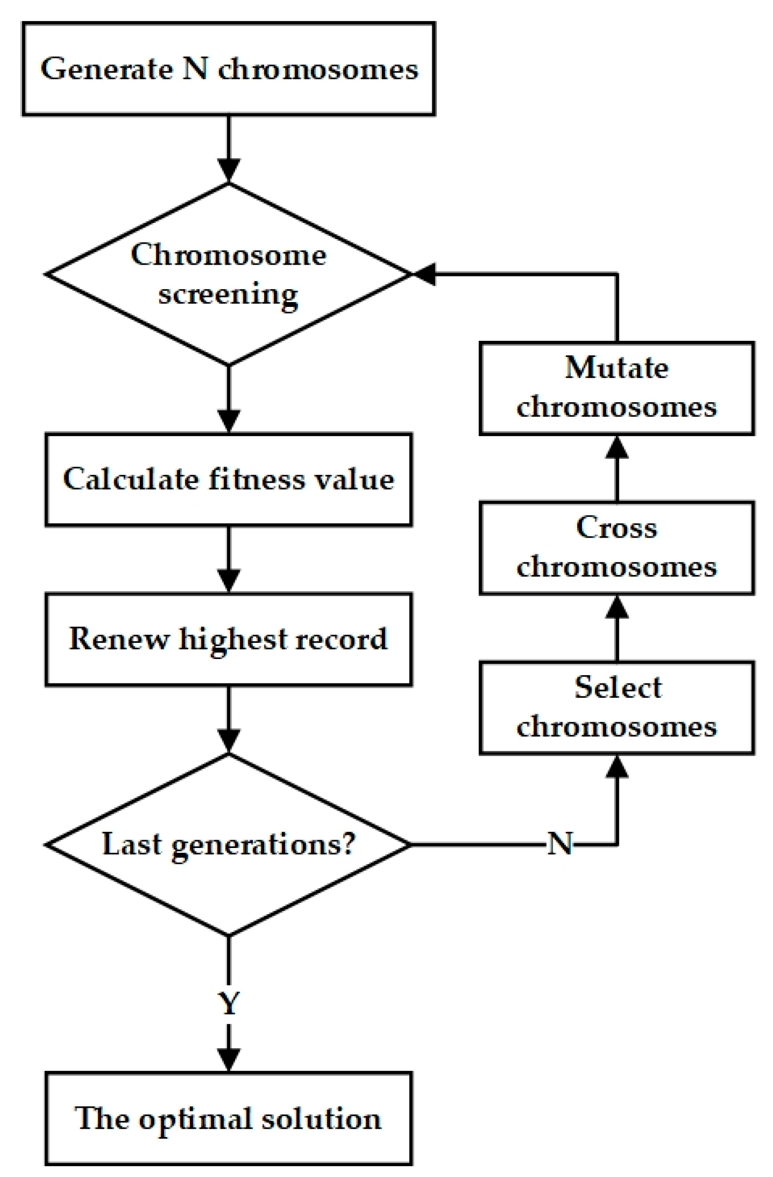
The steps of the algorithm are described as follows (see Figure 4):

Step 1: Randomly generate a population as the primary solution;

Step 2: Perform chromosome screening, which means removing individuals from the population that do not meet the constraints in Model (27);

Step 3: Calculate the fitness of each individual, and we define the fitness function as the reciprocal of the objective function:

$$\frac{1}{fitness}={\displaystyle \sum _{i=0}^n\frac{{\displaystyle \sum _{j=0}^n{\displaystyle \sum _{k=1}^m{c}_1{x}_{ijk}d\left(i,j\right)}}}{{[1-ℳ\left\{{\xi }_i\le y_i\right\}]}^l}}+c_2{\displaystyle \sum _{i=0}^n{y}_i};$$

(28)

Step 4: Renew the record of the individuals with the highest fitness;

Step 5: Determine whether the maximum number of generations has been reached. If so, proceed to Step 6; if not, perform genetic manipulation (reproduction, crossover, mutation) to form the population’s next generation, and then return to Step 2;

Step 6: The last reserved individual with the highest fitness is the optimal solution.

5. A Numerical Example

This section provides a numerical example to verify the model’s validity. A spare parts warehouse and 19 locations were developed as part of the network structure. There are five cars ready to transport spare parts.

Table 3. Relevant parameters of spare parts transportation and genetic algorithm.

Parameter	Value
n	19
m	5
$\mathrm{the} \mathrm{order} \cos \mathrm{t} \mathrm{of} \mathrm{each} \mathrm{spare} \mathrm{part} c_1$	6
$\mathrm{the} \mathrm{delivery} \cos \mathrm{t} \mathrm{per} \mathrm{unit} \mathrm{distance} c_2$	1
Z	6
the penalty coefficient l	3
V	1
the number of iterations	5000
the number of chromosomes of each iteration	100
the probability of chromosomal crossover	0.8
the probability of chromosomal mutation	0.8

and

Table 4. Relevant parameters of spare parts delivery sites.

i	Location	Ƶ(ai, bi, ci)			${\mathit{N}}_{\mathit{i}}$	${\mathit{R}}_{\mathit{i}}$	${\mathit{\alpha }}_{\mathit{i}}$	${\mathit{\beta }}_{\mathit{i}}$	${\mathit{\gamma }}_{\mathit{i}}$	${\mathit{A}}_{\mathit{i}}$
		${\mathit{a}}_{\mathit{i}}$	${\mathit{b}}_{\mathit{i}}$	${\mathit{c}}_{\mathit{i}}$
1	88.91	47	126	221	30	210	0.9	0.9	0.85	0.8
2	43.11	116	133	178	40	120	0.9	0.9	0.85	0.8
3	44.90	21	88	163	30	180	0.9	0.9	0.85	0.8
4	11.37	7	62	109	18	80	0.9	0.9	0.85	0.8
5	80.67	18	130	202	28	120	0.9	0.9	0.85	0.8
6	22.85	40	102	196	25	180	0.9	0.9	0.85	0.8
7	66.44	60	110	160	30	90	0.9	0.9	0.85	0.8
8	72.61	15	75	115	20	80	0.9	0.9	0.85	0.8
9	52.24	72	140	208	28	90	0.9	0.9	0.85	0.8
10	45.61	110	162	206	34	100	0.9	0.9	0.85	0.8
11	14.69	104	137	182	30	80	0.9	0.9	0.85	0.8
12	34.33	57	104	135	20	90	0.9	0.9	0.85	0.8
13	82.30	100	110	160	25	120	0.9	0.9	0.85	0.8
14	57.19	28	95	182	25	100	0.9	0.9	0.85	0.8
15	62.32	55	105	175	25	140	0.9	0.9	0.85	0.8
16	29.40	18	140	222	30	130	0.9	0.9	0.85	0.8
17	72.46	59	103	135	25	140	0.9	0.9	0.85	0.8
18	62.10	98	150	202	40	120	0.9	0.9	0.85	0.8
19	30.52	59	118	185	35	110	0.9	0.9	0.85	0.8

illustrate the key parameters for the entire model.

Questionnaires are designed to obtain experience data from professionals in the field of spare parts. The spare parts demand for each site is derived from the questionnaire data. Considering that the demand is always non-negative for such an uncertain parameter, we think uncertain variables with positive endpoints better match the reality. We believe that following zigzag uncertainty distribution is a good choice for the demand because it better reflects the statistical data and simplifies the calculation. The parameters can then be calculated. Therefore, the uncertainty distribution of the uncertain spare parts demand ${\xi }_i$ of site i could be represented in Equation (29)

$${\Phi }_i\left(x\right)=\{\begin{array}{ll}0\hfill & \left(x\le a_i\right)\hfill \\ \frac{x-a_i}{2\left(b_i-a_i\right)}\hfill & \left(a_i\le x\le b_i\right)\hfill \\ \frac{\left(x+c_i-2b_i\right)}{2\left(c_i-b_i\right)}\hfill & \left(b_i\le x\le c_i\right)\hfill \\ 1\hfill & \left(x\ge c_i\right)\hfill \end{array}$$

(29)

which is denoted by $Z\left(a_i,b_i,c_i\right)$, $a_i<b_i<c_i$.

Then, the inverse uncertainty distribution of ${\xi }_i$ is represented below [27].

$${\Phi }_i{}^{-1}\left(\alpha \right)=\{\begin{array}{ll}\left(1-2\alpha \right)a_i+2\alpha b_i\hfill & \left(\alpha <0.5\right)\hfill \\ \left(2-2\alpha \right)b_i+2\left(2\alpha -1\right)c_i\hfill & \left(\alpha \ge 0.5\right)\hfill \end{array}.$$

(30)

The computation time of the algorithm is acceptable. The configuration of the laptop we use is Processor: Intel(R) Core (TM) i7-7500U CPU @ 2.70GHz 2.90 GHz, with RAM: 8.00 GB. The total calculation time for the simulation is around 121.649 s.

Figure 5 and

Table 5. Optimal supply plan: spare parts delivery route diagram for each site.

i	Location	Spare Parts Supply
1	88.91	170
2	43.11	168
3	44.90	130
4	11.37	105
5	80.67	166
6	22.85	167
7	66.44	127
8	72.61	94
9	52.24	161
10	45.61	181
11	14.69	178
12	34.33	129
13	82.30	145
14	57.19	134
15	62.32	132
16	29.40	164
17	72.46	122
18	62.10	183
19	30.52	147

depict the results. For this spare parts transportation task, we may acquire the optimal supply strategy as shown below. Table 5 shows the supply amounts of spare parts from the warehouse to 19 sites, with a minimum total cost of 5232.7647. Figure 5a depicts the spare parts delivery route planned for each site.

6. Discussion and Conclusions

In this paper, we proposed a spare parts transportation route optimization method under the premise of systematically considering the supportability indicators. In the research of comprehensive support, this paper provided a new direction for improving the equipment support capability and spare parts management efficiency. Due to the existing uncertainty in demand for new equipment spare parts, we proposed using uncertainty theory to reasonably quantify the site’s demand.

This study analyzed the existing problems in spare parts support. On the one hand, the chaos of transportation route planning complicates spare parts management and reduces support efficiency. On the other hand, the irrational allocation of spare parts supply raises the cost of spare parts support. In order to solve these problems, this paper proposed combining the previous research on transportation route optimization with the supportability requirements of the spare parts supply system.

In addition, in the early stages of equipment renewal, the historical data of many new spare parts are inadequate, which often happens in the operation and support phases of equipment. In this case, there are deviations in our understanding of the actual spare parts demand, and the spare parts demand prediction model based on these deviations is likely to be subject to epistemic uncertainty. In the presence of such uncertainty, using a random distribution to fit the spare parts demand is inaccurate because it does not conform to the premise of probability theory—the Law of Large Numbers. In order to address this issue, we devised a more reasonable allocation method in the face of uncertain spare parts demand.

In this study, the uncertain spare parts demand forecast was combined with the vehicle routing problem, and the uncertain chance-constrained spare parts routing planning model of a multi-site equipment maintenance support system was established. In order to solve this model, we used a genetic algorithm. This method effectively incorporates supportability indicators into the route planning model to some extent. It is possible to strike a balance between the supportability requirements and the overall cost. It introduces a novel concept for the transportation of spare parts, which is critical to the equipment support system.

However, there are some limitations to our work. In our modeling process, only the transportation cost of a single variety of spare parts was considered. The transportation of various types of spare parts will be involved in the actual operation of the support system. The capacity limitation of the transport vehicles, as well as the existence of different types of transport vehicles, were not taken into account in the transportation process assumed by the model [41]. At the same time, the process of choosing the supportability indicators might be a little straightforward. In practice, many factors, such as delay time, are involved in supporting indicators, and the calculation is also more complicated. Further analysis of relevant indicators to make them more applicable to reality is also a pressing issue that must be addressed.

Green supply chain research has gradually become a trend in recent years. People are becoming more aware of the importance of environmental protection. Mohtashami et al. presented a bi-objective NLP model for a green supply chain network with reverse logistics consideration. They reduced transportation and waiting time in loading centers, which reduced energy consumption and the environmental impact of the transportation fleet [42]. Kechagias et al. also proposed an urban freight transportation system to reduce emissions [43]. We believe that it may be a good plan to add consideration of factors affecting environmental quality to our study. Furthermore, in this model, we only considered the demand of each site that has the greatest impact on the optimization results, treating it as an uncertain variable. There are some other uncertain factors that can be considered in practical applications. Similarly, given the limitations of the genetic algorithm, the solution algorithm of our model has further research value [44]. Thus far, despite the fact that we proposed and demonstrated the feasibility of a new theoretical method, we still need to investigate its application effects.