Article

MoHydroLib: An HMU Library for Gas Turbine Control System with Modelica

1
School of Energy and Power Engineering, Beihang University, Beijing 100191, China
2
Beihang Hangzhou Innovation Institute Yuhang, Hangzhou 310023, China
3
Systems Engineering Research Institute, Beijing 100094, China
*
Author to whom correspondence should be addressed.
Symmetry 2022, 14(5), 851; https://doi.org/10.3390/sym14050851
Submission received: 12 March 2022 / Revised: 16 April 2022 / Accepted: 18 April 2022 / Published: 20 April 2022

Abstract

:
Modelica is an open-source, object-oriented equation-based modeling language. It is suitable for describing sophisticated dynamic systems (symmetry/asymmetry) as it uses mathematical acausal equations to express physical characteristics. The hydraulic mechanical units (HMU) of gas turbine engine control systems couple the contents of mechanical, hydraulic, symmetry, and other multidisciplinary fields. This paper focuses on the Modelica description method of those HMU models. The content of this work is threefold: firstly, the division form of basic elements in HMU is defined, and the method for describing these element models with Modelica is proposed; secondly, the organization of the element models is defined by using the inheritance characteristics of Modelica, and a lightweight (small code scale) component model is designed; and finally, the causal/acausal connections are designed according to bond graph theory, and the elements and components are integrated into a prototype modeling library. In this paper, the modeling library is verified by comparing simulation results of five typical HMU subsystem models with commercial modeling and simulation software.

1. Introduction

Hydraulic mechanical units (HMU) are widely used in aviation. For aeroengine control systems, HMUs are an important control actuator that contain lots of symmetry/asymmetry geometry, such as actuating pistons and special-shaped orifices. Its characteristics directly affect the design of control systems [1]. Therefore, it is necessary to carry out modeling and simulation research on HMUs.
The modeling and simulation of HMUs usually proceed in two ways: turning to mature commercial modeling and simulation software or studying and developing from the very beginning. Most of the underlying code of commercial software is invisible due to patents, copyright, and other problems, so it is difficult to understand the full process of modeling. In addition, commercial software is wide-ranging, and its organization is huge and complex, so its learning threshold is high. However, developing new HMU modeling tools expends a lot of time on learning, design, and testing. Therefore, the increasing demand for lightweight HMU modeling tool, which is easy to understand and use, is obvious.
In the field of modeling and simulation tools of HMUs, typical commercial software includes the simcenter AMESim of Siemens [2], Bathfp for hydraulic systems simulation developed by Bath University, UK [3], and the simulation software EASY5 for control systems developed by the MSC company (California, USA) [4]. In addition, there are some self-developed software tools. Min Xu et al. designed a set of HMU component model libraries in Matlab/Simulink and verified it on a certain aeroengine [5]. Marquis Favre W. et al. developed a planar mechanical modeling library based on AMESim and verified it on a planar seven-body mechanism test example [6,7]. Yuejun Xiao et al. developed an open-ended hydraulic module library based on the objected-oriented Visual Basic language [8]. W. Borutzky et al. introduced a library of hydraulic components, which was still under development [9]. There are also other authors devoting themselves to modeling and simulation of different fields [10,11,12,13]. However, both mature commercial software and self-developed modeling tools have some problems, such as being difficult to comprehend, requiring complex operations, having complicated functions, and being on a huge scale.
To solve the problems above, this paper proposed an HMU modeling library (MoHydroLib (Beijing, China)) based on Modelica. Modelica is an open-source dynamic modeling language suitable for large-scale, complex, and multidisciplinary physical systems. It describes the object through physical equations, and the model based on the equation descriptions is easy to understand in principle. Modelica uses equations to describe the working characteristics of different types of engineering components, and these components can be easily combined into subsystems, systems, and even architectural models [14]. This organization avoids code redundancy and can be used to design lightweight models. Modelica supports the solution of hybrid differential-algebraic equations, which has advantages for the solution of complex dynamic systems [15]. In addition, Modelica is an open-source language and supports the functional mock-up interface (FMI) protocol. The modeling library based on this language has a wider range of uses and can be applied to multi-platform and multi-domain co-simulation [16,17].
The main contributions of this paper are summarized as follows:
  • To lower the threshold for hydraulic system modeling, we developed a simple but powerful library with Modelica for gas turbine control systems, which is easy to access, easy to use, and easy to reshape;
  • We achieved strong compatibility by designing casual/acausal connections, where multi-platform and multi-domain co-simulation are supported;
  • We reduced code lines significantly through devising inheritance relationships and achieved this lightweight library.
The structure of the manuscript is as follows. Section 2 of this paper gives the basic design idea and connection organization process of the modeling library. The application examples of five typical HMU subsystems modeled by MoHydroLib are presented in Section 3, and their implementation functions and the verification of simulation results are discussed. Section 4 gives the summary of this paper.

2. Design of the Library

This section describes the design process of elements, components, and connections in MoHyroLib. Firstly, this section realizes the element design based on the physical equation description of HMU. Secondly, the component design is completed by utilizing the inheritance characteristics of Modelica, which can effectively reduce code redundancy. Finally, the acausal interface is defined by selecting acausal variable pairs in the HMU through applying bond graph theory, and the causal interface corresponding to the FMI interface protocol is used for exporting the packaging module or importing a C/C++ packaging module from other software to realize the co-simulation of multiple platforms.

2.1. Theory and Element Description

The core of HMUs is the control chamber and moving body [18]. The working theory of the control chamber is to control the pressure by changing the flow passing the inlet and outlet, and then determine the opening with the change of pressure. The pressure that acts on the moving body can alter its acceleration, speed, and displacement. The HMU can be divided into corresponding element types according to different functions, mainly including the orifice element, piston element, boundary element, and system element.

2.1.1. Orifice Element

The orifice element is one of the basic elements in HMUs. It can be used for throttling. It is a kind of hydraulic resistor, and its calculation principle is based on the Bernoulli equation [18]. The flow through the orifice is calculated from the pressure difference before and after it. The description equation is shown in Formula (1).
{ Δ P = P 1 P 2 Q 1 = s i g n ( Δ P ) k v 2 | Δ P | / ρ A Q 1 = Q 2
where P 1 and P 2 are the pressures before and after the orifice, respectively, k v represents the flow coefficient of the orifice, A is the flow area of the orifice, Q represents the volume flow rate through orifice and subscripts 1 and 2 indicate the inlet and outlet of this orifice.
Based on Formula (1), the displacement x p of the moving body and the opening u n d e r l a p of the orifice are introduced to obtain the orifice element with shielding. This element can be further subdivided into a circular orifice, a circular orifice with shielding and a special-shaped orifice with shielding.

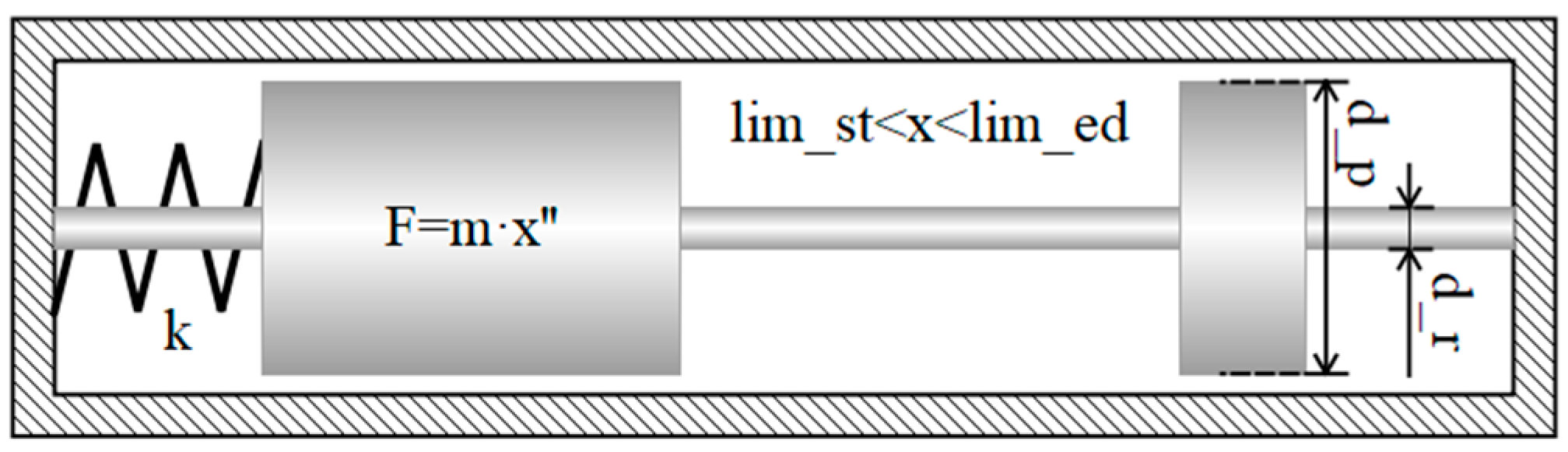
2.1.2. Piston Element

The piston element can also be called a hydraulic cylinder; it is used for converting from hydraulic to mechanic energy. The main function of this element is to calculate the variables related to motion in the HMU. It calculates the acceleration, velocity, and displacement of the mass block according to the hydraulic pressure, spring force and friction. The equations it utilizes refer to Newton’s second law. The positive and negative of the external force calculation are related to the action direction of the corresponding component force. In this element, the force consistent with the positive direction of the displacement of the moving body is defined as positive, and vice versa. The diagram view of this element in the library is shown in Figure 1, and the description equation of it can be seen in Formula (2).
m x ¨ = P l A l P r A r ( k x + F 0 ) c f x ˙
where x , x ˙ and x ¨ represent the displacement, velocity and acceleration of the piston, respectively, m is the mass of piston, P and A are the pressure and pressed area of the control chamber, the subscripts l and r represent the left and right control chamber, k is the stiffness of the spring, F 0 is the pre-tightening force of the spring, and c f represents the coefficient of viscous friction.

2.1.3. Boundary Element

Boundary elements mainly refer to chamber elements and various pressure sources. The operating principle of chamber elements is depicted in Figure 2, and the equation they utilize is described by the pressure differential equation shown in Formula (3). The practical model designed in this paper considers the influence of volume change caused by the moving body as the volume flow rate Q v = A × x ˙ .
d P c d t = B V 0 Q
As can be seen in Figure 2, P c is the pressure of chamber, B is the bulk module of the working medium, V 0 is the volume of chamber, A is the pressed area, and Q is the volume flow rate. The boundary elements in the library also include various pressure sources. These pressure sources defined in this paper include the P source and pressure and the P-m source. The output pressure of the P source can be specified, and the output pressure and mass flow of the P-m source can be specified simultaneously. The function of the pressure source is to provide pressure to the HMU system, which is generally used as the input of other hydraulic components.

2.1.4. System Element

This element is used to define the type of medium working in the HMU, and it is described by some inherent characteristic parameters of the medium, such as the dynamic viscosity n u , bulk modulus B , and density ρ .

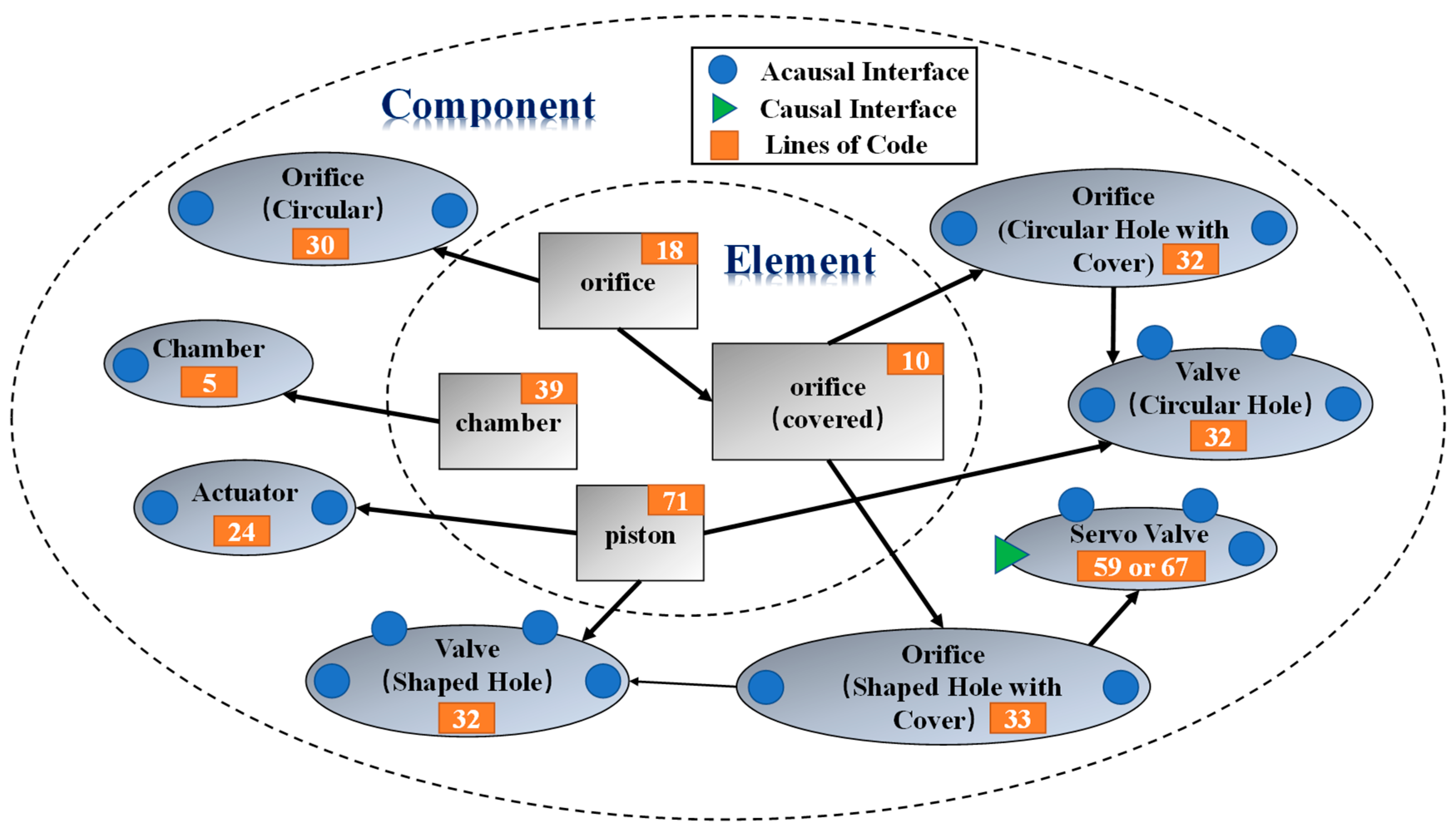
2.2. Component and Inheritance Relationship

In Section 2.1, several different basic elements are designed according to the working theory of HMU. In this section, the organization relationship between elements and the design of components in MoHydroLib is presented. The general organization form of the elements and components is shown in Figure 3.
As can be seen in Figure 3, the library inherits or extends the element model by utilizing the inheritance characteristics of Modelica and adds interactive interfaces to form the component model. The total code of the model library applying this design method is only 452 lines, which is lightweight.

2.2.1. Orifice Component

On inheriting the orifice element, the orifice component introduces five parameters: the maximum flow coefficient c k v m x , the orifice diameter d , the number of orificse n , the hydrodynamic viscosity n u and the critical flow number l a m c . These parameters are associated with the flow coefficient k v and flow area A in the orifice element by an equation, as shown in Formula (4), and the interface is introduced as the input and output port to form a circular orifice component, as shown in Figure 4
{ k v = tanh 32 | Δ P | ρ d n u l a m c c k v m x A = π 4 d 2 × n
The orifice component with a cover can be divided into a circular orifice with a cover and a special-shaped orifice with a cover, as shown in Figure 5. The core of these two kinds of orifices inherits the orifice element with a cover.
The major difference between the two components lies in the different ways of calculating the flow area according to the opening. The calculation of the circular hole is determined by the formula, while the special-shaped orifice is obtained by an a priori interpolation table from the opening to the flow area.

2.2.2. Valve Component

This component couples hydraulics and mechanics by inheriting the orifice element and the piston element. The variation in pressure in the control chamber (port_left and port_right) is converted to the variation in flow in the orifice. Valve components are divided into round hole valves and special-shaped hole valves according to their different orifice types, and the difference between these valves is only the inheritance type of the orifice component. The calculation of motion in valves is inherited from the piston element. The diagram view of a special-shaped hole valve is shown in Figure 6.

2.2.3. Actuator Component

This component is used for implementing control commands by converting hydraulic flow to the actuating force. The actuator component inherits the codes of the piston element and introduces the external load force F p s h to participate in the calculation of displacement, velocity, and acceleration of the moving body. The diagram view of it is shown in Figure 7.

2.2.4. Servo Component

The servo component in MoHydroLib mainly refers to an electro-hydraulic servo valve, which regulates the opening according to the input current. This component realizes conversion from an electrical signal to hydraulic flow. Its motion calculation is different from the piston element, but the flow calculation can still inherit the special-shaped orifice component with a covering.
There are two position three-way valves (HSV23) and three position four-way valves (HSV34) in MoHydroLib. They have similar structures and calculation methods. The diagram views of HSV23 and HSV34 are shown in Figure 8 and Figure 9, respectively.

2.3. Connection Relationship

In order to facilitate the transmission of data and the exchange between designed elements and components, it is necessary to define the input and output interfaces for them. Modelica is an equation-oriented language, and MoHydroLib presented in this paper provides an object-oriented modeling method. This paper carries out interface design based on bond graph theory and combines these two different modeling concepts [19].
Bond graph theory describes the system through power flow and defines three different analogies: signals, components, and connections [20]. This section focuses on describing how to express the connection relationship in an integral system. In order to explain this expression, the concept of causality needs to be introduced: derivative operators need to know the future behavior, while this is numerically impossible [20]. Therefore, causality requires that the integration of variables is calculated by discrete addition, and the flow or unit power is not calculated by the differential form of variable integration; that is, the signal transmission in the system is directional.
According to whether the direction of signal transmission needs to be predetermined, the description of the connection relationship is divided into acausal connection and causal connection. In the MoHydroLib presented in this paper, acausal connection refers to the connection relationship between components and elements, and the power flow on these connections does not need to specify the direction in advance, while causal connection refers to the connection relationship between components or elements and the external environment, other objects, etc. The power flow on these connections needs to specify the direction, as shown in Figure 10.

2.3.1. Acausal Connections

The power flow on the acausal connection does not need to specify the direction. This paper describes the acausal connection by defining the form of the acausal interface. Bond graph theory usually employs a pair of variables to indicate power, such as unit mass work e ( t ) and mass flow Q m . The product of these two variables is power P h . These variable pairs used in this paper are pressure P and volume flow rate Q . The product of the two variables is power, as shown in Formula (5).
P h ( t ) = P ( t ) Q ( t )
As these two variables can be used to describe power, they can serve as an intermediary for the interaction of information between elements and components. This intermediary is defined as an acausal interface. The connection between two acausal interfaces is an acausal connection. If multiple connections are connected to the same acausal interface, the acausal interface is called a junction. Based on bond graph theory [21], the junctions in the model are considered to have the following characteristics:
  • The pressure on each bond/connection connected to the junction is equal:
    P 1 = P 2 = = P n ;
  • The algebraic sum of volume flow of all bonds/connections is zero:
    Q 1 + Q 2 + + Q n = 0 .
For this kind of junction with equal pressure and a zero algebraic sum of the volume flow rate, the pressure needs to be given by other components other than the junction, that is, the boundary elements (chamber and pressure source) in the MoHydroLib. Therefore, the pressure and volume flow rate are used as an acausal interface for the interaction between elements and components, and the data transmission and interaction between components and the external environment are completed through the causal interface in the built-in library of Modelica. An example of causal/acausal connection is shown in Figure 11.
As shown in Figure 11, this example is the electro-hydraulic servo metering subsystem. The circular port includes pressure sources, which are acausal interfaces. The connections of two acausal interfaces are acausal connections. The formation of an acausal connection in the figure includes one-to-one and one-to-many. The data transmission between HMU components can be realized through these acausal interfaces. The triangular port in the figure is the causal interface, which is used to receive the external servo control current.

2.3.2. Causal Connections

Causal connections refers to those connections with clear directionality in MoHydroLib. In this paper, it is only used to represent the input and output interfaces between elements or components in the library and the external environment or other objects. Causal connection directly uses the input and output interface in the Modelica library. At present, the causal interface in the connection of elements and components in MoHydroLib only exists in the external command input of the specified pressure source in the boundary component and the control current input of the servo component. Causal connections are applicable to the type of connection (energy, information flow) that must specify the data direction. There is a clear sequence of calculations or solutions between any two elements or components connected.
In addition, causal connections also include connections with other software. The models constructed by elements or components in MoHydroLib can use the causal interface as the interaction interface with the model in other platforms. The model can also generate an FMU package file based on the FMI interface protocol and call it in other software. However, the FMU file generated in this way can only use the first-order Euler method by default, which is difficult to use to solve some complex dynamic systems. Therefore, packaging the models of other software and calling them under the platform supporting Modelica is an alternative way. For example, after generating the source code of a model, it can be packaged into a DLL file with a C/C++ compiler, and then the DLL file can be called through OpenModelica. In this way, the DAE solver provided by OpenModelica can be utilized.

3. Application Example

Aiming at the HMUs in the control systems of gas turbine engines, this chapter gives several model examples of typical HMU subsystems, including constant pressure valve subsystems, safety valve subsystems, differential pressure valve subsystems, servo metering subsystems and single-port chamber high-frequency dynamic simulation subsystems. The simulation results of these typical subsystem models are compared with the results of a model constructed by commercial HMU modeling software. Since these subsystems can hardly be tested independently, their functions are not verified experimentally. There are some experimental verifications carried out by others comparing simulation results (using the same commercial software) with the experimental data [22,23,24]. Therefore, the simulation of this manuscript is rational and reliable to some extent. Despite the simplicity (452 lines of code in total), the strong ability of the library is verified in this section, compared with the well-known commercial software.

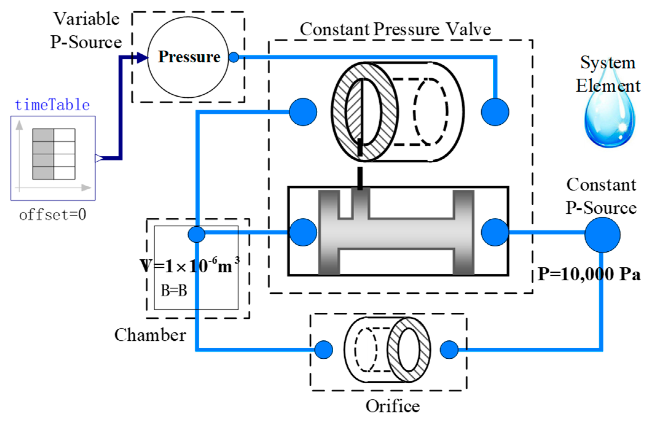
3.1. Constant Pressure Valve Subsystem

The constant pressure valve subsystem is a hydraulic component used to maintain the constant control pressure. The structure of the corresponding subsystem is shown in Figure 12.
The inlet pressure of the constant pressure valve is given by a variable pressure source element with a change trend as shown in Figure 13.
The model calculates the outlet control pressure of the constant pressure valve and the displacement of the valve core under the above inlet pressure input conditions.
The simulation results are shown in Figure 14. The constant pressure valve subsystem established by MoHyroLib can realize the basic function, and its simulation results are basically consistent with those of commercial software.

3.2. Safety Valve Subsystem

The safety valve subsystem is a hydraulic component to ensure that the pressure after the pump does not exceed the set safety value when the speed of the fuel pump increases continuously. The structure of the safety valve subsystem is shown in Figure 15.
The trend of the input speed of the pump is shown in Figure 16. The calculated pressure after the pump and the displacement of the safety valve under this input speed is shown in Figure 17.
Comparing the simulation results in Figure 17, the safety valve subsystem established by MoHydroLib can achieve the desired function, and the simulation results are basically consistent with the results of the commercial software.

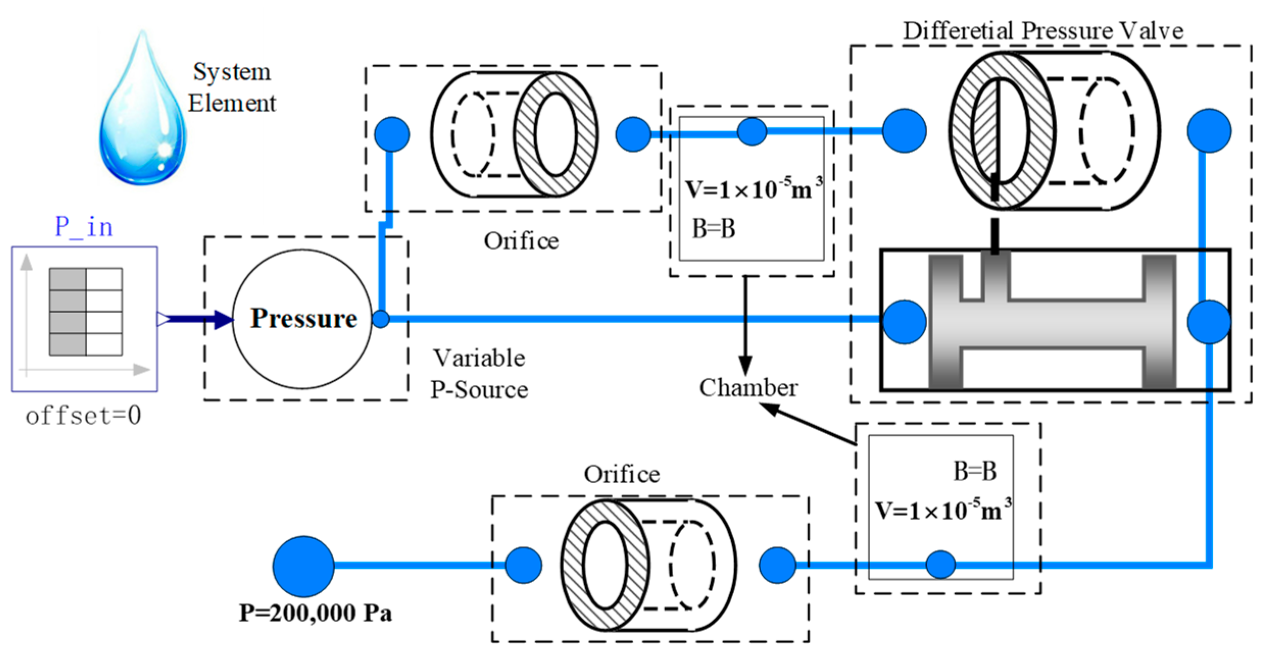
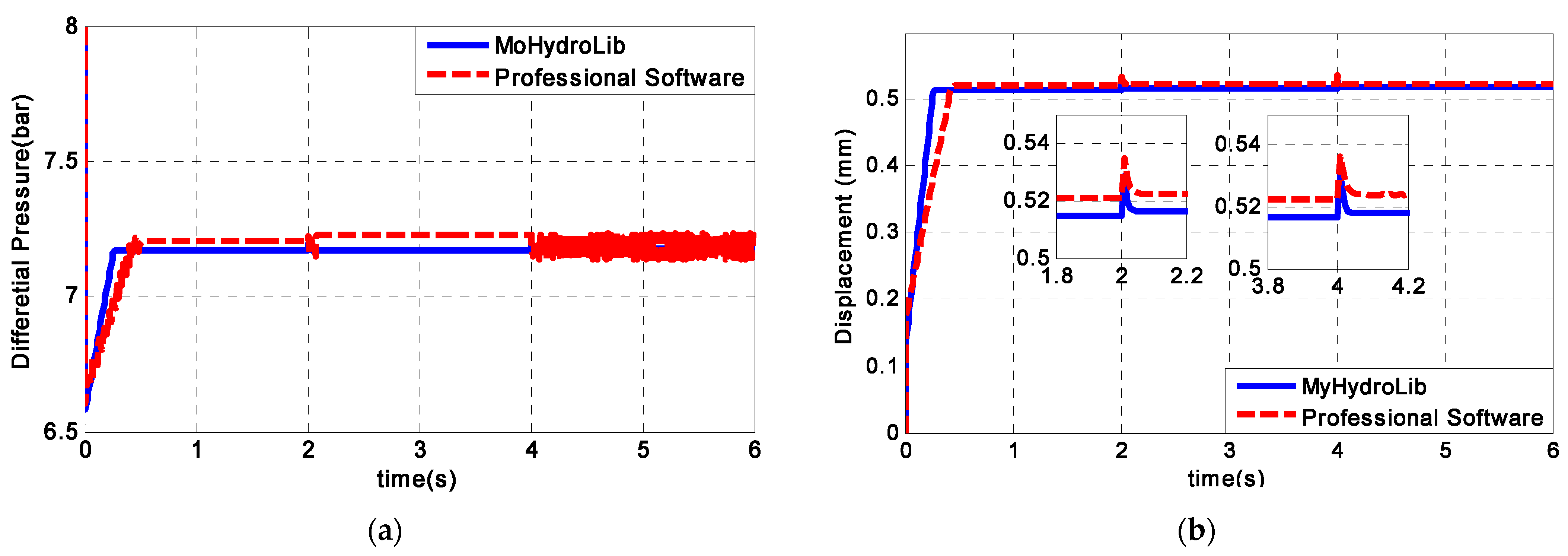
3.3. Differential Pressure Valve Subsystem

The differential pressure valve subsystem is a hydraulic component that maintains the differential pressure at the inlet and outlet of the metering valve within a certain range. The model structure of the subsystem is shown in Figure 18. The change trend of the inlet pressure in the differential pressure valve subsystem is shown in Figure 19a. The model can calculate the outlet pressure (outlet pressure of the metering valve), pressure difference and spool displacement of the valve.
Comparing the simulation results of these two models (Figure 19b and Figure 20), the differential pressure valve subsystem established by MoHydroLib could realize its basic functions, and its simulation results are basically consistent with those of commercial software.

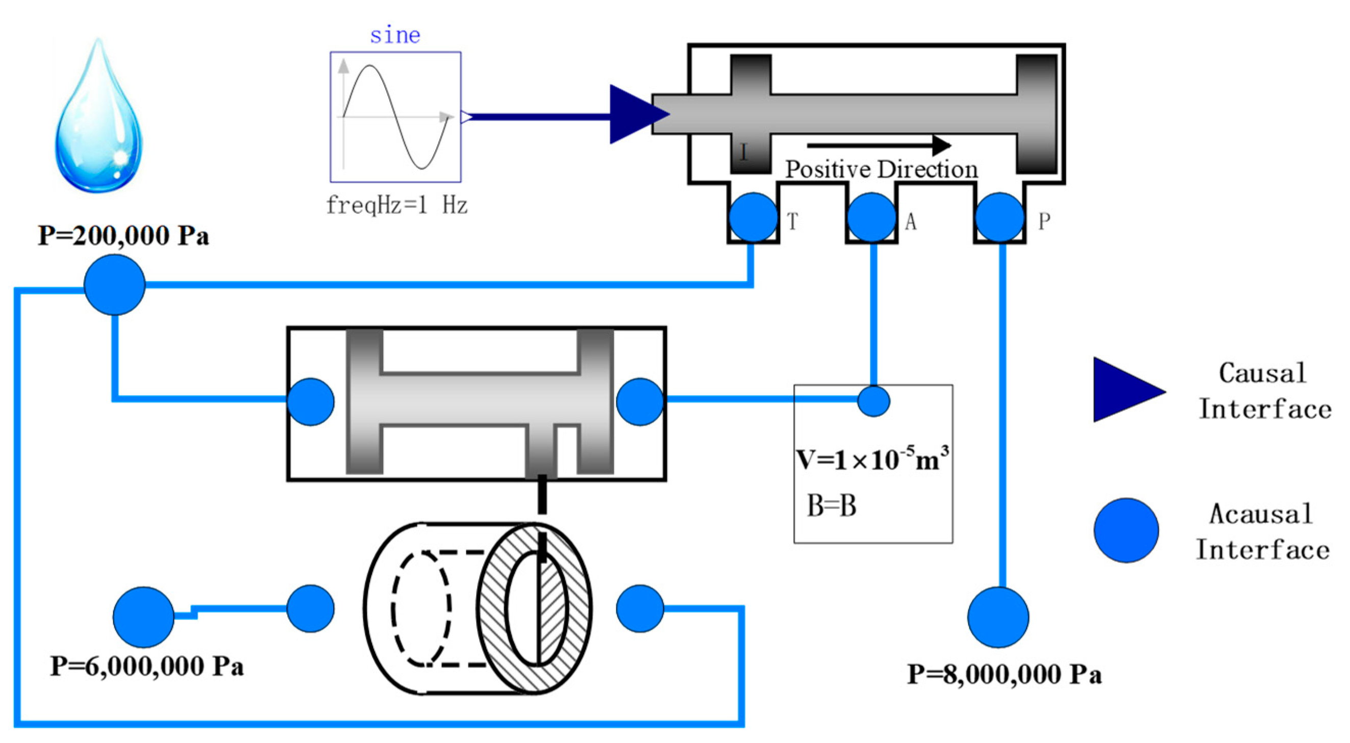
3.4. Servo Metering Subsystem

The servo metering subsystem is the basic hydraulic component of fuel supply system. It uses an electro-hydraulic servo valve to control the flow area of metering valve. Under the closed-loop feedback control, the command tracking of the metering valve displacement is realized. The corresponding subsystem structure is shown in Figure 21.
The change trend in current of servo valve is shown in Figure 22. Under this input condition, the displacement of the metering valve and the outlet metering flow of the subsystem can be calculated, and it is shown in Figure 23. Based on the model structure shown in Figure 21, the displacement closed-loop control of the metering valve is added, and the structure is shown in Figure 24.
Given the displacement command of the closed-loop servo metering subsystem, as shown in Figure 25, the closed-loop displacement response and metering outlet flow of the subsystem can be obtained through model simulation, as can be seen in Figure 26.
Comparing the simulation results of Figure 23 and Figure 26, the servo metering subsystem established by MoHydroLib can realize the basic functions, and the simulation calculation results are basically consistent with the commercial software.

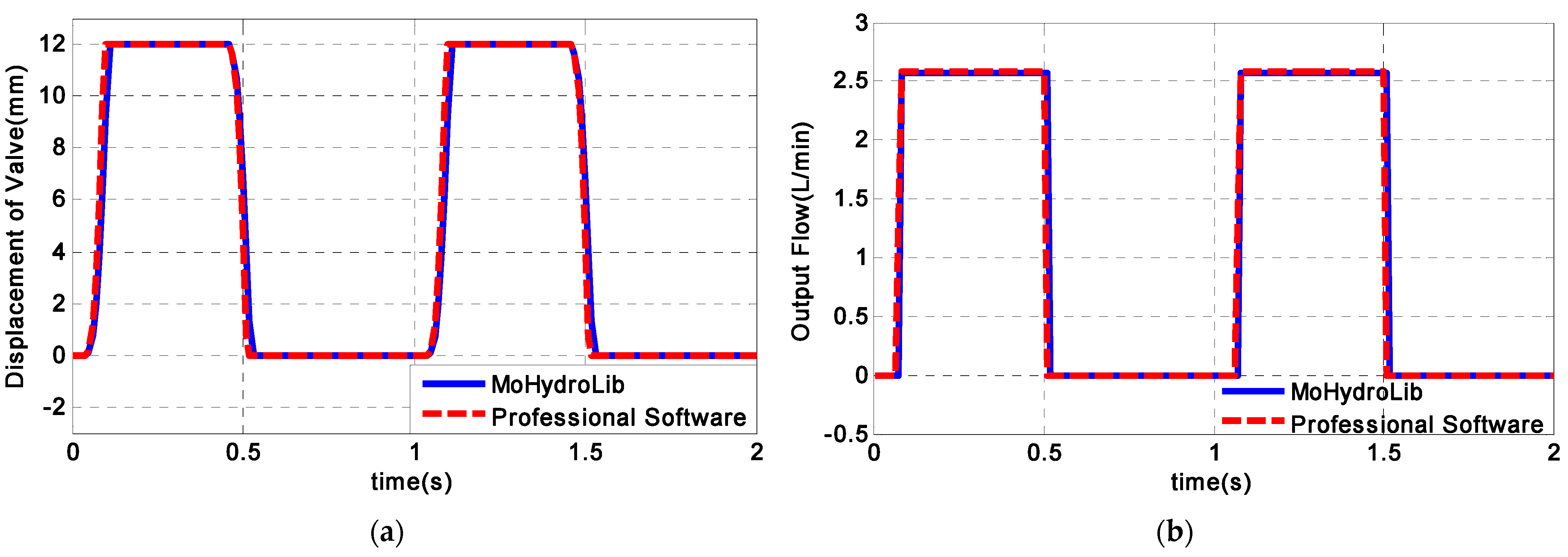
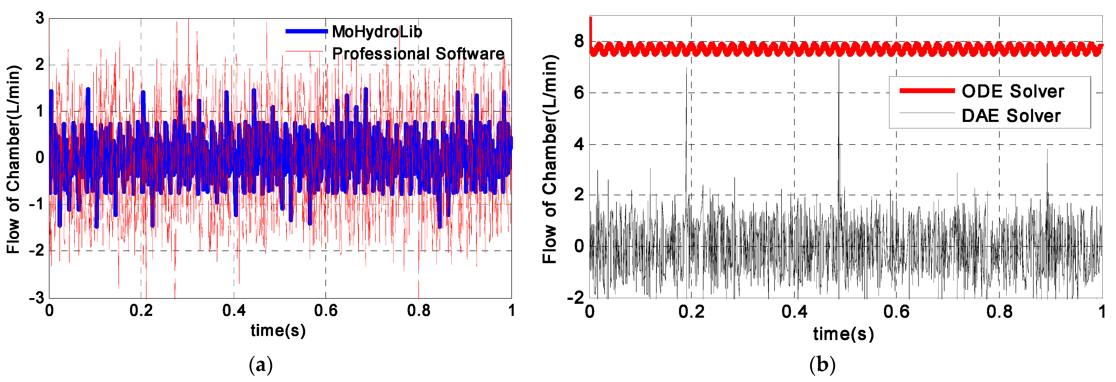
3.5. High Frequency Dynamic Solution Simulation

This section is intended to verify the calculation results of a subsystem shown in Figure 27. The fixed-opening valve component in this subsystem is the substitute for an orifice. According to the assumption of an incompressible working medium, since the volume of the chamber cannot be changed, when the inlet pressure of the orifice changes at high frequency, the inlet flow of the chamber should theoretically be zero. The simulation verifies whether the model can correctly calculate the inlet flow of the chamber under this condition. In this example, the calculation accuracy of different software is uniformly set with 1 × 10 4 . The change of the inlet pressure is shown in Figure 28.
Under the input conditions, the calculation results are shown in Figure 29. The simulation of this example compares the calculation results of OpenModelica, a commercial HMU modeling and simulation software and a commercial mathematical modeling and simulation software. In addition, it compares the calculation results of different solvers (ODE and DAE) in a commercial mathematical modeling and simulation software.
Figure 29 shows that the model flow calculation results based on MoHydroLib are satisfied under the given 1 × 10 4 calculation accuracy, which is close to the calculation results of a commercial HMU modeling and simulation software. When the commercial mathematical modeling and simulation software chooses the ode solver, due to the defects of its computer theory, it leads to incorrect calculation results, while using the DAE solver, the results are basically close to the other two models.

4. Discussion

This manuscript designs a lightweight HMU modeling library based on the Modelica language. The library is mainly applied for the modeling and simulation of HMUs in gas turbine engine control systems. This library completes the description of HMU elements, components and subsystems based on Modelica and devises acausal and causal interfaces to realize the interaction of information between various parts and also make multi-platform co-simulation possible. It has the following advantages:
  • It demonstrates a low threshold; the description of the basic elements in the library is based on the physical equations of the working theory of the HMU, such as Newton’s second law in motion calculation and Bernoulli’s principle in flow calculation, which is easy to understand in principle;
  • It is lightweightl the library adopts the Modelica language and uses the “inheritance” feature of the language. The total code of the modeling library is 452 lines, which is convenient for users to learn, modify and use;
  • It demonstrates a strong simulation capability. It is capable of calculating high-frequency dynamic responses of a single port chamber orifice system, and the simulation results are consistent with the results of a professional HMU modeling and simulation software;
  • It demonstrates good simulation compatibility. The library is implemented in the open-source Modelica language and supports the FMI protocol. It has good compatibility with other software and languages. Meanwhile, it supports the export of FMU format and the import of dynamic link library files for co-simulation calculations.
In the future, further developments based on the modeling library which are not limited to HMUs in gas turbine engine control systems could be considered. The modeling and simulation of sensors, controllers, and the engine itself could also be realized by the Modelica language.

Author Contributions

Conceptualization, Y.L. and S.Y.; methodology, Y.L. and Z.J.; software, Y.L., Z.J., J.L. and W.Z.; validation, X.W., W.Z. and M.Z.; investigation, H.C. and K.M.; resources, S.Y., X.W. and Y.Z.; data curation, H.C., K.M. and Y.Z.; writing—original draft preparation, Y.L.; writing—review and editing, S.Y. and M.Z.; visualization, S.Y.; supervision, X.W.; project administration, X.W.; funding acquisition, X.W. All authors have read and agreed to the published version of the manuscript.

Funding

This research is supported by National Science and Technology Major Project (2017-V-0015-0067) and AECC Sichuan Gas Turbine Establishment Stable Support Project (GJCZ-0011-19).

Institutional Review Board Statement

Not applicable.

Informed Consent Statement

Not applicable.

Data Availability Statement

Not applicable.

Conflicts of Interest

The authors declare no conflict of interest.

References

  1. Padovani, D.; Rundo, M.; Altare, G. The Working Hydraulics of Valve-Controlled Mobile Machines. J. Dyn. Syst. Meas. Control. 2020, 142, 070801. [Google Scholar] [CrossRef]
  2. Simcenter System Simulation. Available online: https://www.plm.automation.siemens.com/global/en/products/simcenter/simcenter-system-simulation.html (accessed on 1 March 2022).
  3. Centre for Power Transmission & Motion Control Software. Available online: https://www.bath.ac.uk/case-studies/centre-for-power-transmission-motion-control-software (accessed on 1 March 2022).
  4. Easy5: Advanced Control & Systems Simulation. Available online: https://www.mscsoftware.com/product/easy5 (accessed on 1 March 2022).
  5. Xu, M.; Wang, X.; De-tang, Z. Simulation on hydromechanical controller of modern aero-engine. J. Aerosp. Power 2009, 24. [Google Scholar] [CrossRef]
  6. Marquis-Favre, W.; Bideaux, E.; Scavarda, S. A planar mechanical library in the AMESim simulation software. Part I: Formulation of dynamics equations. Simul. Model. Pract. Theory 2006, 14, 25–46. [Google Scholar] [CrossRef] [Green Version]
  7. Marquis-Favre, W.; Bideaux, E.; Scavarda, S. A planar mechanical library in the AMESim simulation software. Part II: Library composition and illustrative example. Simul. Model. Pract. Theory 2006, 14, 95–111. [Google Scholar] [CrossRef] [Green Version]
  8. Xiao, Y.; Zhu, J.; Zhang, D. Study on visual modeling and simulation platform of hydraulic system based on bond graph. Proc. SPIE—Int. Soc. Opt. Eng. 2005, 6041, 440–444. [Google Scholar]
  9. Borutzky, W.; Barnard, B.; Thoma, J.U. Describing bond graph models of hydraulic components in Modelica. Math. Comput. Simul. 2000, 53, 381–387. [Google Scholar] [CrossRef]
  10. Zhu, M.; Wang, X. An Integral Type µ Synthesis Method for Temperature and Pressure Control of Flight Environment Simulation Volume. In Proceedings of the ASME Turbo Expo 2017: Turbomachinery Technical Conference and Exposition, Charlotte, NC, USA, 26–30 June 2017. [Google Scholar]
  11. Graeber, M.; Kosowski, K.; Richter, C.; Tegethoff, W. Modelling of heat pumps with an object-oriented model library for thermodynamic systems. Math. Comput. Model. Dyn. Syst. 2010, 16, 195–209. [Google Scholar] [CrossRef]
  12. Pei, X.; Liu, J.; Wang, X.; Zhu, M.; Zhang, L.; Dan, Z. Quasi-One-Dimensional Flow Modeling for Flight Environment Simulation System of Altitude Ground Test Facilities. Processes 2022, 10, 377. [Google Scholar] [CrossRef]
  13. Jiang, Z.; Wang, X.; Chen, H.; Wang, Y. Design of Speed Closed-Loop Control with Variable Pressure Difference Valve for Aero Engine. In Proceedings of the ASME Turbo Expo 2020: Turbomachinery Technical Conference and Exposition, Virtual, Online, 21–25 September 2020. [Google Scholar]
  14. Michael, M.T. Modelica by Example. Available online: https://mbe.modelica.university/front/intro/ (accessed on 2 March 2022).
  15. Modelica Association. Modelica—A Unified Object-Oriented language for PHYSICAL Systems Modeling. Language Spec. v. 3.4. 2017. Available online: https://modelica.org/documents.html (accessed on 2 March 2022).
  16. Pazold, M.; Burhenne, S.; Radon, J.; Herkel, S.; Antretter, F. Integration of Modelica models into an existing simulation software using FMI for Co-Simulation. In Proceedings of the 9th International Modelica Conference, Munich, Germany, 3–5 September 2012. [Google Scholar]
  17. Blochwitz, T. The functional mockup interface for tool independent exchange of simulation models. In Proceedings of the 8th International Modelica Conference, Dresden, Germany, 20–22 March 2011. [Google Scholar]
  18. Si-qi, F. Aeroengine Control (Volume One), 1st ed.; Northwestern Polytechnic University Press: Xi’an, China, 2008; pp. 141–182. [Google Scholar]
  19. Thoma, J.U.; Perelson, A.S. Introduction to Bond Graphs and Their Application. IEEE Trans. Syst. Man Cybern. 1976, 6, 797–798. [Google Scholar] [CrossRef]
  20. Novák, P.; Sindelár, R. Component-Based Design of Simulation Models Utilizing Bond-Graph Theory. IFAC Proc. Vol. 2014, 47, 9229–9234. [Google Scholar] [CrossRef]
  21. Gawthrop, P.J.; Bevan, G.P. Bond-graph modeling. Control. Syst. IEEE 2007, 27, 24–45. [Google Scholar]
  22. Zhao, H.C.; Wang, B.; Ye, Z.F. Study on Co-Modeling Method for Digital Control Fuel Metering Unit. J. Propuls. Technol. 2016, 37, 1752–1758. [Google Scholar]
  23. Zhang, D. Simulating and Experimental Study on Fuel Control System of a Certain Aeroengine. Master’s Thesis, Nanjing University of Aeronautics and Astronautics, Nanjing, China, 1 March 2008. [Google Scholar]
  24. Wang, B.; Zhao, H.; Yu, L.; Ye, Z. Study of Temperature Effect on Servovalve-Controlled Fuel Metering Unit. ASME J. Eng. Gas Turbines Power 2015, 137, 061503. [Google Scholar] [CrossRef]
Figure 1. Diagram view of piston element.
Symmetry 14 00851 g001
Figure 2. Operating principle of chamber.
Symmetry 14 00851 g002
Figure 3. Relationship between element and component.
Symmetry 14 00851 g003
Figure 4. Diagram view of circle orifice.
Symmetry 14 00851 g004
Figure 5. Diagram view of an orifice with a cover. (a) Circular orifice with cover, (b) special-shaped orifice with cover.
Symmetry 14 00851 g005
Figure 6. Diagram view of a special-shaped hole valve component.
Symmetry 14 00851 g006
Figure 7. Diagram view of actuator component.
Symmetry 14 00851 g007
Figure 8. Diagram view of HSV23 component.
Symmetry 14 00851 g008
Figure 9. Diagram view of HSV34 component.
Symmetry 14 00851 g009
Figure 10. Connection relationship illustration.
Symmetry 14 00851 g010
Figure 11. Causal/acausal connection example.
Symmetry 14 00851 g011
Figure 12. Constant pressure valve system.
Symmetry 14 00851 g012
Figure 13. Input port pressure of a constant valve (pressure after pump).
Symmetry 14 00851 g013
Figure 14. The simulation result of ouput pressure and displacement in different modeling tools. (a) Comparison of output port pressure in a constant valve calculated by two modeling tools; (b) comparison of displacement in a constant valve calculated by two modeling tools.
Symmetry 14 00851 g014
Figure 15. Safety valve system.
Symmetry 14 00851 g015
Figure 16. Input speed of the gear pump.
Symmetry 14 00851 g016
Figure 17. The results of the simulation of the displacement and pressure after pump by two modeling tools. (a) Comparison of displacement in he safety valve calculated by two modeling tools. (b) Comparison of pressure after pump calculated by two modeling tools.
Symmetry 14 00851 g017
Figure 18. Differential pressure valve system.
Symmetry 14 00851 g018
Figure 19. Input and outlet fuel pressure of the differential pressure valve. (a) Input fuel pressure of differential pressure valve given by P-source. (b) Comparison of outlet fuel pressure of the differential pressure valve calculated by two modeling tools.
Symmetry 14 00851 g019
Figure 20. The results of the simulation of the differential pressure and displacement by two modeling tools. (a) Comparison of the differential pressure of the metering valve calculated by two modeling tools. (b) Comparison of the displacement in the differential pressure valve calculated by two modeling tools.
Symmetry 14 00851 g020
Figure 21. Servo valve metering system.
Symmetry 14 00851 g021
Figure 22. Input current of the electro hydraulic servo valve in the servo metering subsystem.
Symmetry 14 00851 g022
Figure 23. The results of the simulation of the displacement and ouput flow by two modeling tools. (a) Comparison of the displacement in the metering valve calculated by two modeling tools. (b) Comparison of the flow in the metering valve calculated by two modeling tools.
Symmetry 14 00851 g023
Figure 24. Servo metering subsystem with a close-loop control.
Symmetry 14 00851 g024
Figure 25. Displacement command signal of the metering valve.
Symmetry 14 00851 g025
Figure 26. The results of the simulation of closed-loop displacement and ouput flow by two modeling tools. (a) Comparison of the displacement with a controller calculated by two modeling tools. (b) Comparison of the flow with a controller calculated by two modeling tools.
Symmetry 14 00851 g026
Figure 27. High-frequency dynamic solution subsystem.
Symmetry 14 00851 g027
Figure 28. Input pressure of the orifice in the subsystem.
Symmetry 14 00851 g028
Figure 29. The simulation result of calculated flow by different modeling tools. (a) Comparison of the flow of the chamber calculated by two modeling tools. (b) Comparison of the flow of the chamber calculated by mathematical simulation software using two different solvers.
Symmetry 14 00851 g029
Publisher’s Note: MDPI stays neutral with regard to jurisdictional claims in published maps and institutional affiliations.

