
An Improved SVM-Based Air-to-Ground Communication Scenario Identification Method Using Channel Characteristics


Abstract
:1. Introduction
2. Channel-Characteristic-Based Scenario Identification Model
3. Improved Identification Method
3.1. RT-Based Acquisition of Channel Characteristics
3.2. Training Dataset of Height-Dependent Channel Characteristics
- indicates the proportion of the building area to the total area;
- indicates the average number of buildings per unit area (buildings/km);
- indicates the height of the building according to the Rayleigh distribution, where h can be calculated by
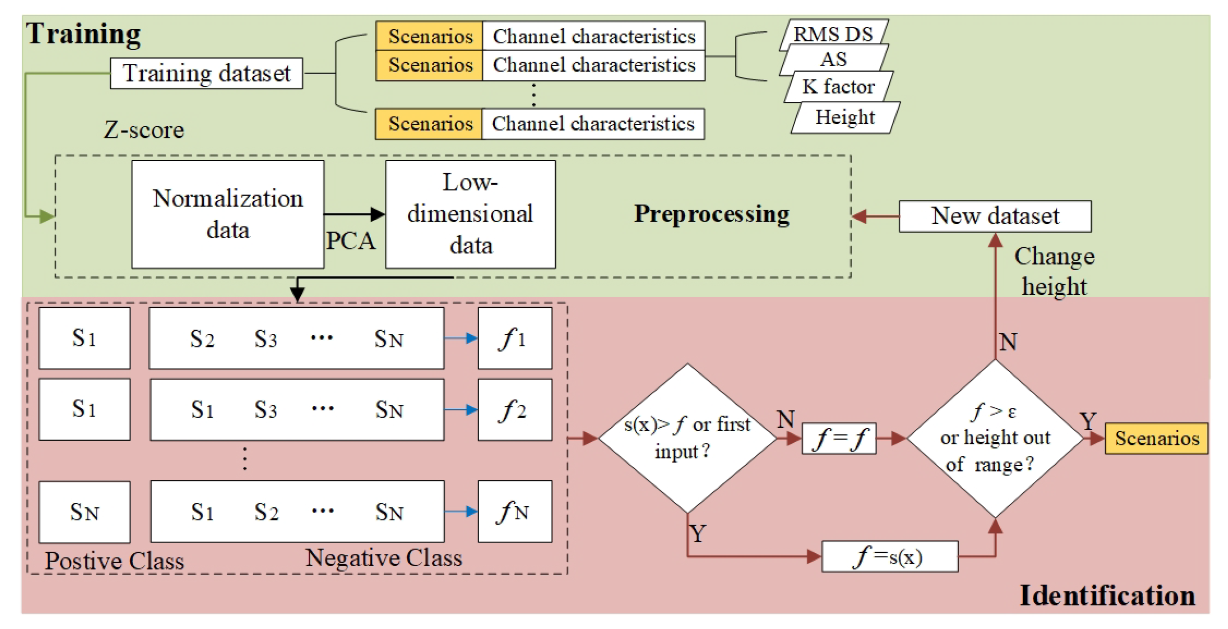
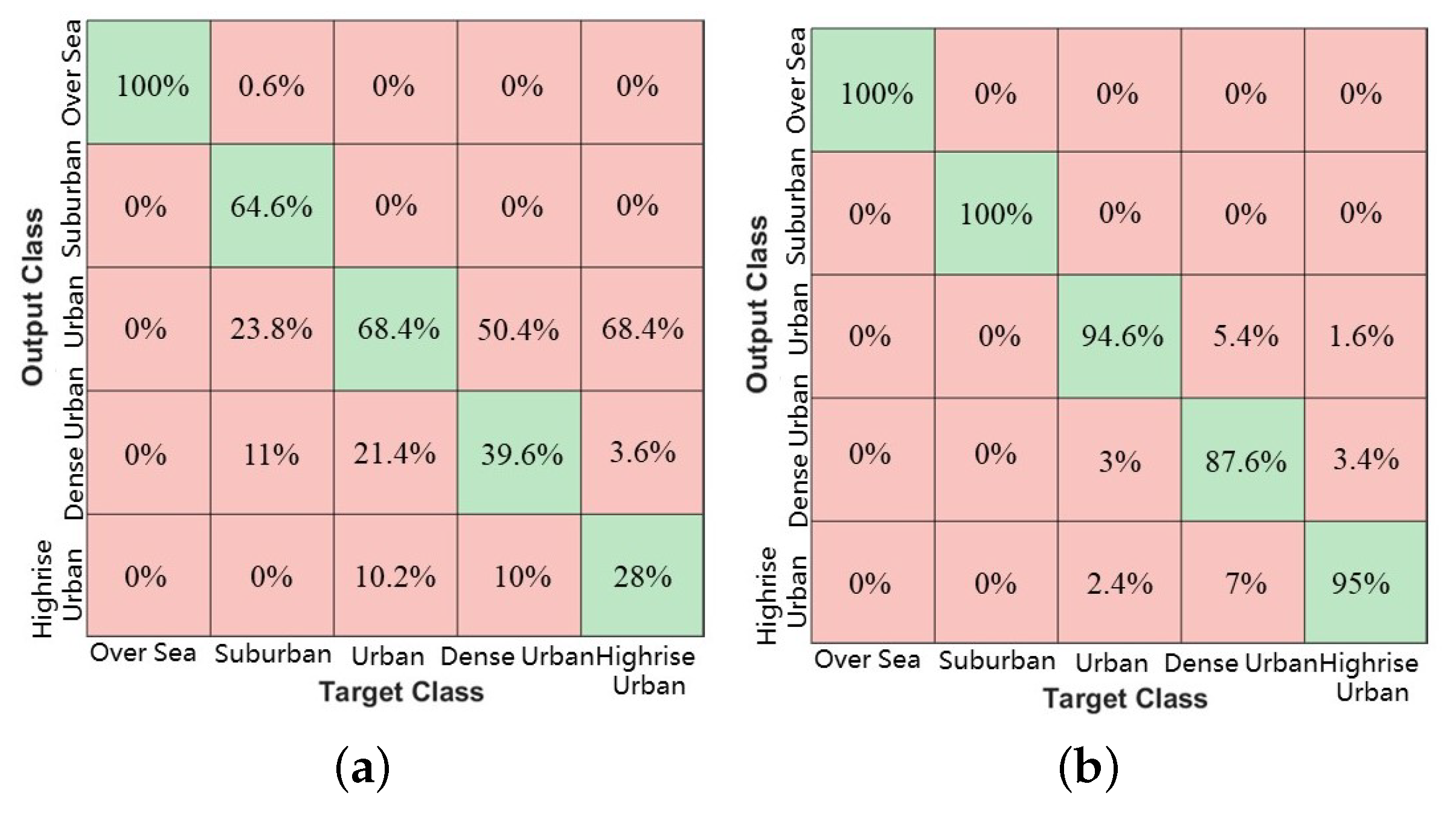
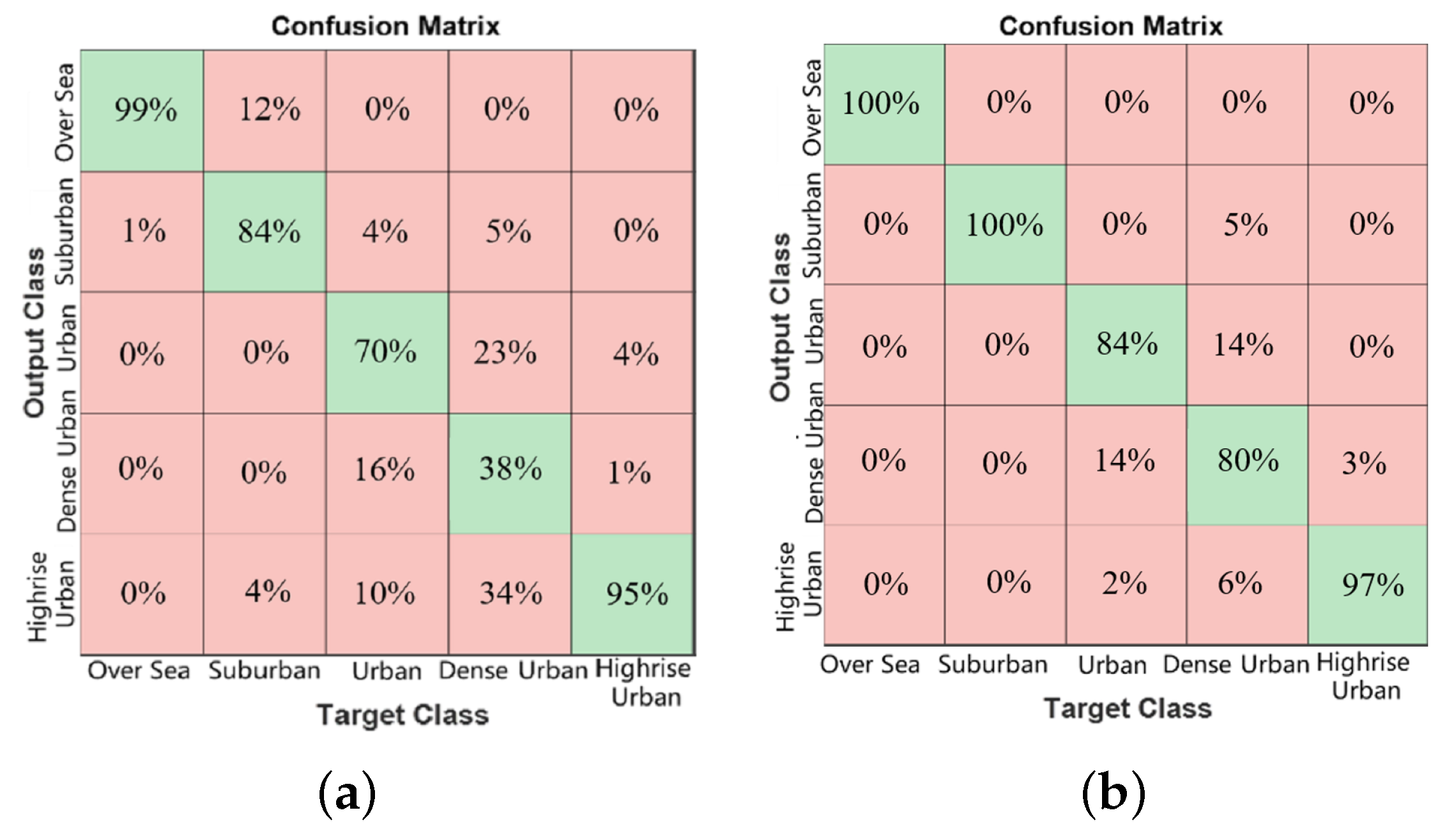
3.3. Height-Integrated Scenario Identification Method
4. Simulation Results and Validation
5. Conclusions
Author Contributions
Funding
Institutional Review Board Statement
Informed Consent Statement
Data Availability Statement
Acknowledgments
Conflicts of Interest
Abbreviations
| UAV | Unmanned aerial vehicle |
| SVM | Support vector machine |
| A2G | Air-to-ground |
| RMS-DS | Root-mean-square delay spread |
| AS | Angle spread |
| RT | Ray tracing |
| 6G | Sixth generation |
| ML | Machine Learning |
| V2V | Vehicle-to-vehicle |
| LOS | Line-of-sight |
| NLOS | Non-line-of-sight |
| GIS | Geographic informaiton system |
| CNN | Convolutional Neural Network |
| BPNN | Back Propagation Neural Network |
| LR | Logistic regression |
| SBR/IM | Shooting and bouncing ray/image |
| AAOA | Angle spread of azimuth angle of arrival |
| AAOD | Angle spread of azimuth angle of arrival |
| EAOA | Angle spread of elevation angle of arrival |
| EAOD | Angle spread of elevation angle of arrival |
| ITU-R | International Telecommunication Union-Radiocommunication Sector |
| PCA | Principal component abalysis |
References
- Alsamhi, S.H.; Gupta, S.K.; Rajput, N.S.; Saket, R.K. Network Architectures Exploiting Multiple Tethered Balloon Constellations for coverage extension. In Proceedings of the 6th International Conference on Advances in Engineering Sciences and Applied Mathematics (ICAESAM), Kuala Lumpur, Malaysia, 21–22 December 2016; pp. 24–29. [Google Scholar]
- Giordani, M.; Polese, M.; Mezzavilla, M.; Rangan, S.; Zorzi, M. Toward 6G Networks: Use Cases and Technologies. IEEE Commun. Mag. 2020, 58, 55–61. [Google Scholar] [CrossRef]
- Wang, C.X.; Huang, J.; Wang, H.; Gao, X.; You, X.H.; Hao, Y. 6G Wireless Channel Measurements and Models: Trends and Challenges. IEEE Veh. Technol. Mag. 2020, 15, 22–32. [Google Scholar] [CrossRef]
- Gupta, A.; Gupta, S.K.; Rashid, M.; Khan, A.; Manjul, M. Unmanned aerial vehicles integrated HetNet for smart dense urban area. Trans. Emerg. Telecommun. Technol. 2020, 9, 1–22. [Google Scholar] [CrossRef]
- Gupta, A.; Sundhan, S.; Gupta, S.K.; Alsamhi, S.H.; Rashid, M. Collaboration of UAV & HetNet for better QoS: A Comparative Study. Int. J. Commun. Syst. 2020, 5, 309–333. [Google Scholar]
- Rashid, A.; Sharma, D.; Lone, T.A.; Gupta, S.; Gupta, S.K. Secure Communication in UAV Assisted HetNets: A Proposed Model. In Security, Privacy and Anonymity in Computation Communication and Storage (SpaCCS); Springer: Charm, Switzerland, 2019; pp. 427–440. [Google Scholar]
- Gupta, A.; Sundhan, S.; Alsamhi, S.H.; Gupta, S.K. Review for capacity and coverage improvement in aerially controlled heterogeneous network. In Proceedings of the International Conference on Optical and Wireless Technologies, Jaipur, India, 10–11 February 2018; pp. 365–376. [Google Scholar]
- Gupta, A.; Gupta, S.K. UAV Aided Fog Network (UAFN): A Proposal Framework for Better QoS. In Proceedings of the 2nd International Conference on Computing and Information Technology (ICCIT), Tabuk, Saudi Arabia, 25–27 January 2022; pp. 265–270. [Google Scholar]
- Sharma, M.; Gupta, A.; Gupta, S.K.; Alsamhi, S.H. Survey on Unmanned Aerial Vehicle for Mars Exploration. Drones 2021, 6, 4. [Google Scholar] [CrossRef]
- Khawaja, W.; Guvenc, I.; Matolak, D.W.; Fiebig, U.C.; Schneckenberger, N. A Survey of Air-to-Ground Propagation Channel Modeling for Unmanned Aerial Vehicles. IEEE Commun. Surv. Tutor. 2019, 21, 2361–2391. [Google Scholar] [CrossRef] [Green Version]
- Zeng, Y.; Zhang, R.; Lim, T.J. Wireless Communications with Unmanned Aerial Vehicles: Opportunities and Challenges. IEEE Commun. Mag. 2016, 54, 36–42. [Google Scholar] [CrossRef] [Green Version]
- Huang, C.; He, R.; Ai, B.; Molisch, A.F.; Lau, B.K.; Haneda, K.; Liu, B.; Wang, C.X.; Yang, M.; Oestges, C.; et al. Artificial intelligence enabled radio propagation for communications-Part II: Scenario identification and channel modeling. IEEE Trans. Antennas Propag. 2022; in press. [Google Scholar] [CrossRef]
- He, R.; Renaudin, O.; Kolmonen, V.; Haneda, K.; Zhong, Z.; Ai, B.; Hubert, S.; Oestges, C. Vehicle-to-vehicle radio channel characterization in crossroad scenarios. IEEE Trans. Veh. Technol. 2016, 65, 5850–5861. [Google Scholar] [CrossRef]
- Zhong, Z.; Ai, B.; Hong, W.; Ding, J. Study on the Propagation Scenario Classification of the High-speed Railway GSM-R System based on GIS. In Proceedings of the 5th IET International Conference on Wireless, Mobile and Multimedia Networks (ICWMMN 2013), Beijing, China, 12–15 June 2013; pp. 306–310. [Google Scholar]
- Morocho-Cayamcela, M.E.; Maier, M.; Lim, W. Breaking Wireless Propagation Environmental Uncertainty with Deep Learning. IEEE Trans. Wirel. Commun. 2020, 19, 5075–5087. [Google Scholar] [CrossRef]
- Greenberg, E.; Bar, A.; Klodzh, E. LOS Classification of UAV-to-Ground Links in Built-Up Areas. In Proceedings of the IEEE International Conference on Microwaves, Antennas, Communications and Electronic Systems (COMCAS 2019), Tel Aviv, Israel, 4–5 November 2019; pp. 1–5. [Google Scholar]
- Zhang, J.; Salmi, J.; Lohan, E.S. Analysis of kurtosis-based LOS/NLOS identification using indoor MIMO channel measurement. IEEE Trans. Veh. Technol. 2013, 62, 2871–2874. [Google Scholar] [CrossRef] [Green Version]
- Tang, P.; Zhang, J.; Molisch, A.F.; Smith, P.J.; Shafi, M.; Tian, L. Estimation of the K-factor for temporal fading from single-snapshot wideband Measurements. IEEE Trans. Veh. Technol. 2019, 68, 49–63. [Google Scholar] [CrossRef]
- Huang, C.; Molisch, A.F.; He, R.; Wang, R.; Zhong, Z. Machine learning-enabled LOS/NLOS identification for MIMO systems in dynamic environments. IEEE Trans. Wirel. Commun. 2020, 27, 1292–1304. [Google Scholar] [CrossRef]
- Li, H.; Li, Y.; Zhou, S.; Wang, J. Wireless Channel Feature Extraction via GMM and CNN in the Tomographic Channel Model. J. Commun. Inf. Netw. 2017, 2, 41–51. [Google Scholar] [CrossRef] [Green Version]
- Yang, M.; Ai, B.; He, R.; Shen, C.; Wen, M.; Huang, C.; Li, J.; Ma, Z.; Chen, L.; Li, X.; et al. Machine-Learning-Based Scenario Identification Using Channel Characteristics in Intelligent Vehicular Communications. IEEE Trans. Intell. Transp. 2021, 22, 3961–3974. [Google Scholar] [CrossRef]
- Zhou, T.; Wang, Y.; Wang, C.X.; Salous, S.; Liu, L.; Tao, C. Multi-Feature Fusion Based Recognition and Relevance Analysis of Propagation Scenes for High-Speed Railway Channels. IEEE Trans. Veh. Technol. 2020, 69, 8107–8118. [Google Scholar] [CrossRef]
- AlHajri, M.I.; Ali, N.T.; Shubair, R.M. Classification of Indoor Environments for IoT Applications: A Machine Learning Approach. IEEE Antennas Wirel. Propag. 2018, 27, 2164–2168. [Google Scholar] [CrossRef]
- Yang, M.; Ai, B.; He, R.; Chen, L.; Li, X.; Li, J.; Zhang, B.; Huang, C.; Zhong, Z. A Cluster-Based Three-Dimensional Channel Model for Vehicle-to-Vehicle Communications. IEEE Trans. Veh. Technol. 2019, 68, 5208–5220. [Google Scholar] [CrossRef]
- Matolak, D.W.; Sun, R. Air-ground channel characterization for unmanned aircraft systems: The over-freshwater setting. In Proceedings of the Integrated Communications, Navigation and Surveillance Conference (ICNS), Herndon, VA, USA, 8–10 April 2014; pp. 1–5. [Google Scholar]
- Sun, R.; Matolak, D.W. Air-Ground Channel Characterization for Unmanned Aircraft Systems—Part II: Hilly & Mountainous Settings. IEEE Trans. Veh. Technol. 2017, 66, 1913–1925. [Google Scholar] [CrossRef]
- Matolak, D.W.; Sun, R. Air–Ground Channel Characterization for Unmanned Aircraft Systems—Part III: The Suburban and Near-Urban Environments. IEEE Trans. Veh. Technol. 2017, 66, 6607–6618. [Google Scholar] [CrossRef]
- Rodríguez-Piñeiro, J.; Domínguez-Bolaño, T.; Cai, X.; Huang, Z.; Yin, X. Air-to-ground channel characterization for low-height UAVs in realistic network deployments. IEEE Trans. Antennas Propag. 2021, 69, 992–1006. [Google Scholar] [CrossRef]
- Izydorczyk, T.; Tavares, F.M.L.; Berardinelli, G.; Bucur, M.C.; Mogensen, P.E. Angular distribution of cellular signals for UAVs in urban and rural scenarios. In Proceedings of the European Conference on Antenna and Propagation (EUCAP), Krakow, Poland, 31 March–5 April 2019; pp. 1–5. [Google Scholar]
- Cortes, C.; Vapnik, V. Support-vector networks. Mach. Learn. 1995, 20, 273–297. [Google Scholar] [CrossRef]
- Ponte, P.; Melko, R.G. Kernel methods for interpretable machine learning of order parameters. Phys. Rev. B 2017, 96, 205146–205153. [Google Scholar] [CrossRef] [Green Version]
- ITU-R Recommendation P.1410-2 Propagation Data and Prediction Methods for The Design of Terrestrial Broadband Millimetric Aadio Access Systems. Available online: https://www.itu.int/rec/R-REC-P.1410-2-200304-S/en (accessed on 15 April 2003).
- Lever, J.; Krzywinski, M.; Altman, N. Points of significance: Principal component analysis. Nat. Methods 2017, 14, 641–642. [Google Scholar] [CrossRef] [Green Version]
- Lyu, W.; Li, Y.; Liu, Z.; Huang, C.; He, R. A target recognition-based NLOS identification algorithm. In Proceedings of the IEEE International Symposium on Antennas and Propagation and USNC-URSI Radio Science Meeting (APS/USNC-URSI 2019), Atlanta, GA, USA, 7–12 July 2019; pp. 2093–2094. [Google Scholar]
- Huang, C.; Molisch, A.F.; Wang, R.; Tang, P.; He, R.; Zhong, Z. Angular Information-Based NLOS/LOS Identification for Vehicle to Vehicle MIMO System. In Proceedings of the IEEE International Conference on Communications Workshops (ICC Workshops 2019), Shanghai, China, 20–24 May 2019; pp. 1–6. [Google Scholar]


| Parameter | Value |
|---|---|
| Scenario | Over-sea, Suburban, urban, dense urban, high-rise urban |
| Area ration of scatters | 0.005, 0.1, 0.3, 0.5, 0.5 |
| Number of scatters (km2) | 50, 750, 500, 300, 300 |
| Height of scatters | 4 m, Rayleigh distribution of 8, 15, 20, 50 |
| Size of scatters | 20 m × 5 m, 11.6 m × 11.6 m, 24.5 m × 24.5 m, 40.5 m × 40.5 m, 40.5 m × 40.5 m |
| Frequency | 2.4 GHz |
| Bandwidth | 100 MHz |
| Antenna type | Half-wave dipole antenna |
| Transmitting power | 20 dBm |
| Height of TX | 1.7 m |
| Number of TX | 10 |
| Height of RX | Between 10 m to 210 m with 2 m intervals |
| Number of RX | 3000 |
| Scenario | (ns) | K | ||||
|---|---|---|---|---|---|---|
| Over-sea | 4.6127 | 6.6838 | 0.9793 | 2.1590 | 2.1805 | 76.53 |
| Suburban | 102.3164 | 6.3169 | 0.7497 | 1.059 | 1.065 | 77.9331 |
| Unbran | 127.4503 | 5.3237 | 16.1668 | 18.1029 | 21.7193 | 68.5246 |
| Dense Urban | 143.4544 | 5.2331 | 14.2822 | 18.3465 | 19.0873 | 63.8681 |
| Highrise Urban | 125.8363 | 5.3187 | 37.6931 | 31.4001 | 43.3032 | 43.0069 |
| Data Sets | Datapoints Number |
|---|---|
| Total data sets | 3000/3000/3000/3000/3000 |
| Training data | 1800/1800/1800/1800/1800 |
| Testing data | 1200/1200/1200/1200/1200 |
| Scenario | Over-Sea | Suburban | Urban | Dense Urban | High-Rise Urban |
|---|---|---|---|---|---|
| K factor + RMS DS | 100% | 100% | 79% | 70% | 85% |
| K factor + RMS DS + AS | 100% | 100% | 84% | 80% | 97% |
| PL + K factor + RMS DS + AS | 100% | 100% | 80% | 77% | 96% |
| Data Sets | Datapoints Number |
|---|---|
| 1.7 m | 100/100/100/100/100 |
| 3 m | 100/100/100/100/100 |
| 4 m | 100/100/100/100/100 |
| 5 m | 100/100/100/100/100 |
| 6 m | 100/100/100/100/100 |
Publisher’s Note: MDPI stays neutral with regard to jurisdictional claims in published maps and institutional affiliations. |
© 2022 by the authors. Licensee MDPI, Basel, Switzerland. This article is an open access article distributed under the terms and conditions of the Creative Commons Attribution (CC BY) license (https://creativecommons.org/licenses/by/4.0/).
Share and Cite
Zhu, G.; Liu, Y.; Mao, K.; Zhang, J.; Hua, B.; Li, S. An Improved SVM-Based Air-to-Ground Communication Scenario Identification Method Using Channel Characteristics. Symmetry 2022, 14, 1038. https://doi.org/10.3390/sym14051038
Zhu G, Liu Y, Mao K, Zhang J, Hua B, Li S. An Improved SVM-Based Air-to-Ground Communication Scenario Identification Method Using Channel Characteristics. Symmetry. 2022; 14(5):1038. https://doi.org/10.3390/sym14051038
Chicago/Turabian StyleZhu, Guyue, Yuanjian Liu, Kai Mao, Jingyi Zhang, Boyu Hua, and Shuangde Li. 2022. "An Improved SVM-Based Air-to-Ground Communication Scenario Identification Method Using Channel Characteristics" Symmetry 14, no. 5: 1038. https://doi.org/10.3390/sym14051038
APA StyleZhu, G., Liu, Y., Mao, K., Zhang, J., Hua, B., & Li, S. (2022). An Improved SVM-Based Air-to-Ground Communication Scenario Identification Method Using Channel Characteristics. Symmetry, 14(5), 1038. https://doi.org/10.3390/sym14051038