Article

A Multi-Objective Cellular Memetic Optimization Algorithm for Green Scheduling in Flexible Job Shops

School of Computer Science, China University of Geosciences, Wuhan 430074, China
*
Author to whom correspondence should be addressed.
Symmetry 2022, 14(4), 832; https://doi.org/10.3390/sym14040832
Submission received: 17 March 2022 / Revised: 9 April 2022 / Accepted: 13 April 2022 / Published: 18 April 2022
(This article belongs to the Section Computer)

Abstract

:
In the last 30 years, a flexible job shop scheduling problem (FJSP) has been extensively explored. Production efficiency is a widely utilized objective. With the rise in environmental awareness, green objectives (e.g., energy consumption) have received a lot of attention. Nevertheless, energy consumption has received little attention. Furthermore, controllable processing times (CPT) should be considered in the field of scheduling, because they are closer to some real production. Therefore, this work investigates a FJSP with CPT (i.e., FJSP-CPT) where asymmetrical conditions and symmetrical constraints increase the difficulty of problem solving. The objectives of FJSP-CPT are to minimize simultaneously the maximum completion time (i.e., makespan) and total energy consumption (TEC). First of all, a mathematical model of this multi-objective FJSP-CPT was formulated. To optimize this problem, a novel multi-objective cellular memetic optimization algorithm (MOCMOA) was presented. The proposed MOMOA combined the advantages of cellular structure for global exploration and variable neighborhood search (VNS) for local exploitation. At last, MOCMOA was compared against other multi-objective optimization approaches by performing experiments. Numerical experiments reveal that the presented MOCMOA is superior to its competitors in 15 instances regarding three commonly used performance metrics.

1. Introduction

With the increasing enhancement of environmental consciousness, green manufacturing has attracted wide attention from both academia and industry. Green manufacturing is an important component to realize the harmonious coexistence of mankind and nature, which has become a new trend and requirement among manufacturing enterprises. Shop scheduling, as a crucial part of manufacturing systems, has played a decisive role in green manufacturing [1,2]. Specifically, a reasonable scheduling rule can effectively ameliorate the environmental problem and achieve the effect of energy conservation and emission reduction [3]. Therefore, it is essential to design a rational shop scheduling technique to reach a target of green production in manufacturing systems.
Recently, many studies on the green scheduling of manufacturing systems have been conducted. Furthermore, Gahm et al. [4] and Gao et al. [5] gave an overview of green or energy-efficient scheduling in production manufacturing systems, respectively. In brief, the relevant research is roughly classified into three types of green scheduling problems: (1) green scheduling in a flow shop environment; (2) green scheduling in a job shop environment; and (3) green scheduling in a flexible job shop environment. Regarding the green scheduling in a flow shop environment, Mansouri et al. [6] and Liu et al. [7] addressed green scheduling in a flow shop for minimizing makespan and energy consumption. Lu et al. [8] studied green scheduling in a permutation flow shop using a backtracking search algorithm. Li et al. [9] solved a hybrid flow shop scheduling problem (HFSP) with total energy consumption (TEC) and makespan objectives. Lu et al. [10] investigated a HFSP considering three objectives, i.e., noise pollution, makespan, and TEC. Li et al. [11] and Zuo et al. [12] addressed an energy-efficient HFSP with objectives of total tardiness, makespan, and TEC. Wang et al. [13] studied a HFSP to minimize makespan and TEC. Lei et al. [14] invented a teaching–learning-based optimization algorithm for solving a HFSP with makespan, total tardiness, and TEC, simultaneously. Gong et al. [15] addressed an energy-efficient HFSP with worker flexibility. Zhang et al. [16] designed a multi-objective optimization algorithm based on decomposition to address a HFSP with makespan and energy consumption criteria. Concerning the green scheduling of job shops, May et al. [17] adopted a multi-objective genetic algorithm to deal with an energy-efficient job shop scheduling problem (JSP). Zhang et al. [18] presented a hybrid multi-objective genetic algorithm for solving a JSP with total weighted tardiness and TEC. Yin et al. [19] investigated an energy-efficient JSP considering TEC and noise pollution. Giglio et al. [20] solved an integrated lot-sizing and energy-efficient JSP. He et al. [21] investigated a JSP, which aims to minimize makespan, total tardiness, and TEC. Abedi et al. [22] focused on a JSP to minimize the total weighted tardiness and TEC. Regarding the green scheduling in flexible job shops, Yin et al. [23] established a mathematical model for the low-carbon flexible job shop scheduling problem (FJSP). Zhang et al. [24] proposed an effective gene expression programming algorithm for solving an energy-efficient FJSP. Luo et al. [25] presented a grey wolf optimizer for solving a green FJSP. Duan et al. [26] investigated a FJSP with objectives of minimizing makespan and TEC. Li and Lei [27] designed an imperialist competitive algorithm for a green FJSP with objectives of makespan, total tardiness, and TEC.
Although green scheduling in various shop environments has been extensively studied, job processing times are usually deemed to be constant. In realistic production, job processing times are controlled by expending extra resources (e.g., energy resource and human resource). Thus, controllable processing times (CPT) should be considered in green shop scheduling problems, which are much closer to real-world manufacturing. Compared to other shop types, FJSP with CPT (FJSP-CPT) is much more difficult. FJSP-CPT has been confirmed to be NP-hard since it was first raised [28]. Nevertheless, green FJSP-CPT is still unexplored so far. Thus, we attempt to investigate a green FJSP-CPT with objectives of minimization of makespan and TEC. Green FJSP-CPT requires considering collaborative optimization between benefit and environment criteria. Obviously, it is a multi-objective shop scheduling problem. Many optimization approaches have been employed to address such multi-objective combinatorial optimization issues [29]. These methods include a prior method and posterior method. Concerning the prior method, a multi-objective issue is merged into a mono-objective problem by adopting a weighted sum method. However, this method has several disadvantages, such as obtaining prior information of problems and concealing the trade-off relationship among all objectives. Concerning the prior method, a Pareto-based posterior approach can generate some trade-off or non-dominated solutions and shows the coupling relation among objectives without prior information. However, it is hard to obtain new non-dominated solutions at each iteration. To solve this problem, the fitness of each individual involving the raw fitness value and density indicator is used in this work. Meanwhile, a local search can significantly improve the performance in solving shop scheduling problems. Additionally, to alleviate premature convergence, one population is divided into many sub-populations by utilizing a cellular structure. Therefore, a multi-objective cellular memetic algorithm (MOCMOA) was designed to handle this energy-efficient FJSP-CPT. Numerical experiments reveal that the proposed MOCMOA can solve this problem well.
Energy-efficient FJSP-CPT has not been researched yet. This problem aims to gain some non-dominated solutions between makespan and TEC. Therefore, the novelties of this paper are as follows:
(1)
Concerning the problem model, a mathematical model of energy-efficient FJSP-CPT was formulated.
(2)
Concerning the optimization algorithm, a new multi-objective cellular memetic optimization algorithm (MOCMOA) was designed to handle this energy-efficient FJSP-CPT.
(3)
Concerning the experiment, experiments were performed to prove the effectiveness of the MOCMOA.
The rest of the article is structured as follows. Section 2 summarizes the problem statement and a mathematical model for energy-efficient FJSP-CPT. Section 3 details a proposed MOCMOA approach. Section 4 presents numerical results. This work is concluded in Section 5.

2. Problem Statement and Mathematical Model

This section provides a problem statement and mathematical model.

2.1. Problem Statement

In general, a multi-objective optimization problem (MOP) for minimization is formulated below:
min f ( x ) = min [ f 1 ( x ) , f 2 ( x ) , , f m ( x ) ] x = ( x 1 , x 2 , x n ) R
where x is one feasible solution and R is the search space. Suppose a and b are two different solutions. The solution a will dominate b , if and only if f i ( a ) f i ( b ) for each index i { 1 , , m } and f l ( a ) < f l ( b ) for at least one index l { 1 , , m } . One solution x R will be one Pareto optimal point if it is not dominated by anyone else. All Pareto optimal solutions satisfying the above conditions are called Pareto optimal set (PS*). The objective point of PS* is named the optimal Pareto front (PF*).
Energy-efficient FJSP-CPT is stated briefly: A set of n jobs ( i = 1 , 2 , , n ) are handled on a set of m machines . Each job i has a set of n i operations { O i , 1 , O i , 2 , , O i , j , , O i , n i } , in which O i , j is the j -th operation of the job i . Each operation O i , j can be handled on any one of the available machines i j . Furthermore, the processing time of each operation can be controlled by adjusting energy resources. However, it will cause an increase in energy consumption. The objectives of FJSP-CPT are minimization of the makespan and TEC, simultaneously.
Assumptions of the energy-efficient FJSP-CPT are stated below:
(1)
Interruption is not permitted and all machines are in good condition.
(2)
Transportation and setup times are overlooked.
(3)
Machines/jobs are independent of each other.

2.2. Mathematical Model

With the above notations, an energy-efficient FJSP-CPT is formulated below.
min f 1 = C m a x = m a x { C i j k | i = 1 , 2 , , n ; j = 1 , 2 , , n i ; k = 1 , 2 , , m }
min   f 2 = T E C = E C w + E C s
Subject to
C i j k C i ( j 1 ) k p i j k a   X i j k j , k ; j = 2 , , n i
S i j k + p i j k a S g h k + L ( 1 Y g h i j k ) ( i , j ) , ( g , h ) , k
E C w = i = 1 n j = 1 n i k = 1 m p i j k a X i j k P k w o r k
E C s = i = 1 n j = 1 n i g = 1 n h = 1 n g k = 1 m ( S i j k C g h k ) Y g h i j P k i d l e
p i j k L p i j k a p i j k U   ( i , j ) , k
k = 1 m X ijk = 1   ( i , j )
Objective (2) and Objective (3) represent the makespan and TEC. Equation (4) confines the operation precedence relation of the same job. Equation (5) imposes that each machine can handle at most one job at any a time. Equations (6) and (7) show the total work energy consumption and total idle energy consumption, respectively. Equation (8) provides the bound of the processing times of each operation. Equation (9) guarantees that one operation can only be handled by one machine at a time.

3. Proposed Multi-Objective Optimization Approach

We provide a framework of MOCMOA for the energy-efficient FJSP-CPT in this part. The main steps of MOCMOA are explained in detail.

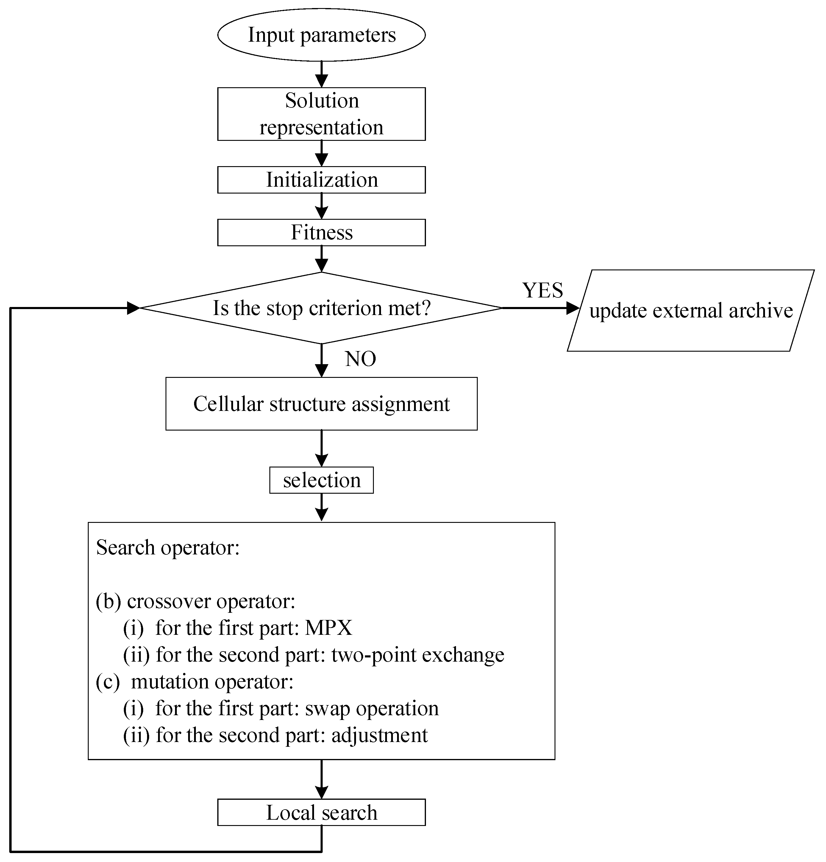
3.1. Framework of MOCMOA

In this paper, a MOCMOA is presented to address this energy-efficient FJSP-CPT. The flowchart of the MOCMOA is depicted in Figure 1.
The main steps of MOCMOA are below.
Step 1: Initialization population: Yield one initial population randomly and establish an external archive (EA) for storing a non-dominated solution set.
Step 2: Fitness: Calculate the fitness values of all the individuals.
Step 3: Cellular structure assignment: Each individual is assigned to one lattice structure, where each individual has its neighbors. Consequently, one population can be classified into many subpopulations.
Step 4: Selection: Select two parents from the population.
Step 5: Update: Choose two good individuals from each sub-population based on fitness. Individuals can only communicate with their neighbors.
Step 5.1: Search operator: The search progress is often directed by crossover and mutation. Refer to Section 3.1.5 for more details.
Step 5.2: Variable Neighborhood Search (VNS): Variable neighborhood structures are used to hunt for promising solutions. For the specific information of VNS, refer to Section 3.1.6.
Step 6: Update EA: If no other solutions in EA can dominate solution x, put this solution into the EA and remove all solutions that are dominated by the solution x. When non-dominated solutions are full of EA, ones with the larger fitness will be deleted.
Step 7: Termination criterion: If the termination condition is satisfied, stop iteration optimization. Otherwise, execute the above iteration.
In MOCMOA, several critical components, including encoding, decoding, initialization, selection, search operator, and local search, are elaborated in the subsequent subsections.

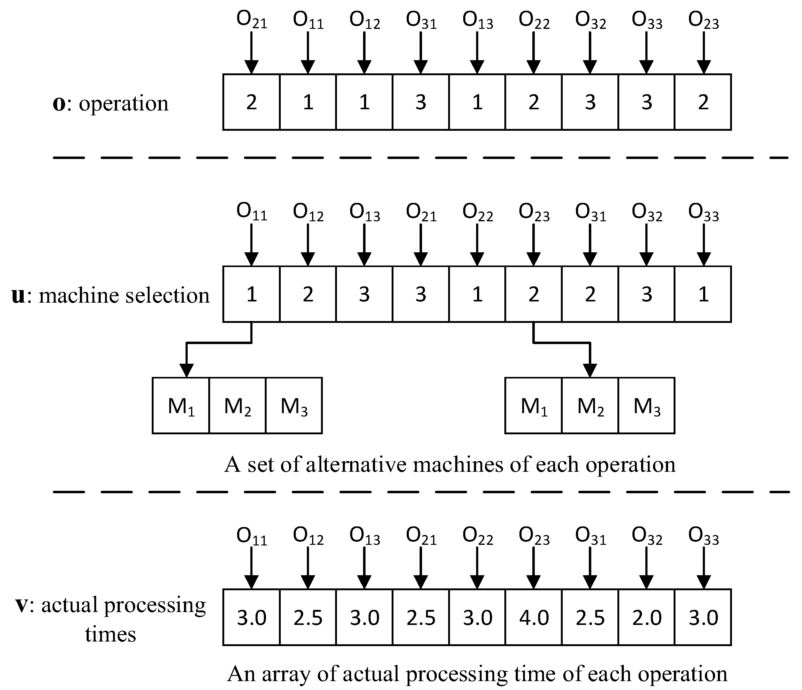
3.1.1. Encoding and Decoding

A three-part-based encoding mechanism is utilized to express one solution representation. The first part o represents an operation vector. The second part u indicates the chosen machine for the operation. The third part v refers to the practical processing times of the operation. The first part o involves the job index, in which job i presents n i times. The second part u indicates an integer vector representing the machine index of each operation. The third part v is a set of real numbers representing the practical processing times of each operation. The total length of three parts is the length of each solution.
To further explain this encoding mechanism, Figure 2 plots this solution representation. The total length of each solution is 27, where the length of each part of this solution is 9. The first part o denotes a list of all operations, i.e., O21-O11-O12-O31-O13-O22-O32-O33-O23. The operation is processed with priority based on its order. The second part u is the index of the machine to process operation. The third part v indicates the actual processing times of each operation on the selected machine.
The decoding mechanism is stated as follows: When one solution is decoded, the first part o is transformed into a list of operations. Then, each operation is handled by one chosen machine according to the second part u . At last, the actual processing times are determined according to the third part v . To be specific, one operation cannot be handled until its adjacent predecessor is completed. [ S x , E x   ] is the idle time interval on the machine k of each operation, where x is the x-th idle time interval of O i j . It satisfies the following condition:
{ m a x { S x , C i , j 1 } + p i j k a E x       i f   j 2 S x + p i j k a E x                                                       i f   j = 1
where O i j can be positioned in the idle time interval [ S x , E x ] , the starting time of O i j is either m a x { S x , C i , j 1 } or S x . If there is no interval on machine k for O i j , O i j will be assigned to the end position of machine k .

3.1.2. Initialization and Cellular Structure Assignment

First, one initial population will be randomly yielded based on the above decoding mechanism and an empty EA built to preserve a non-dominated solution set. One initial population will be grouped into many sub-populations where each individual is allocated in one appointed cellular structure. Each solution in the cellular structure has its state, which is usually related to its neighbors in discrete time steps. The present states of a nearby neighborhood of solutions determine the state of each solution at the following time [30]. As we know, cellular structures contain many types. In this work, we adopt a common cellular structure called the Von Neumann neighborhood.

3.1.3. Fitness

Two entities of each individual, including strength and raw fitness values, should be calculated. Each individual contains its strength value representing the number of individuals that it can dominate. Meanwhile, each individual contains its raw fitness value, which is a summation of the strength values of individuals dominating the present individual. To preserve the individual’s diversity, a density metric is formulated as [31]:
D e n s i t y ( i ) = 1 σ i k + 2
where σ i k is the Euclidian distance from solution i to its k -th closest vicinage, k is set to 1, and the fitness of each solution is calculated below:
F i t n e s s ( i ) = r a w _ f i t n e s s ( i ) + D e n s i t y ( i )

3.1.4. Selection

A tournament selection is employed in this selection operation. One individual with better fitness is selected as one parent (denoted by P1) from two different individuals. The other parent (denoted by P2) is chosen in the same way.

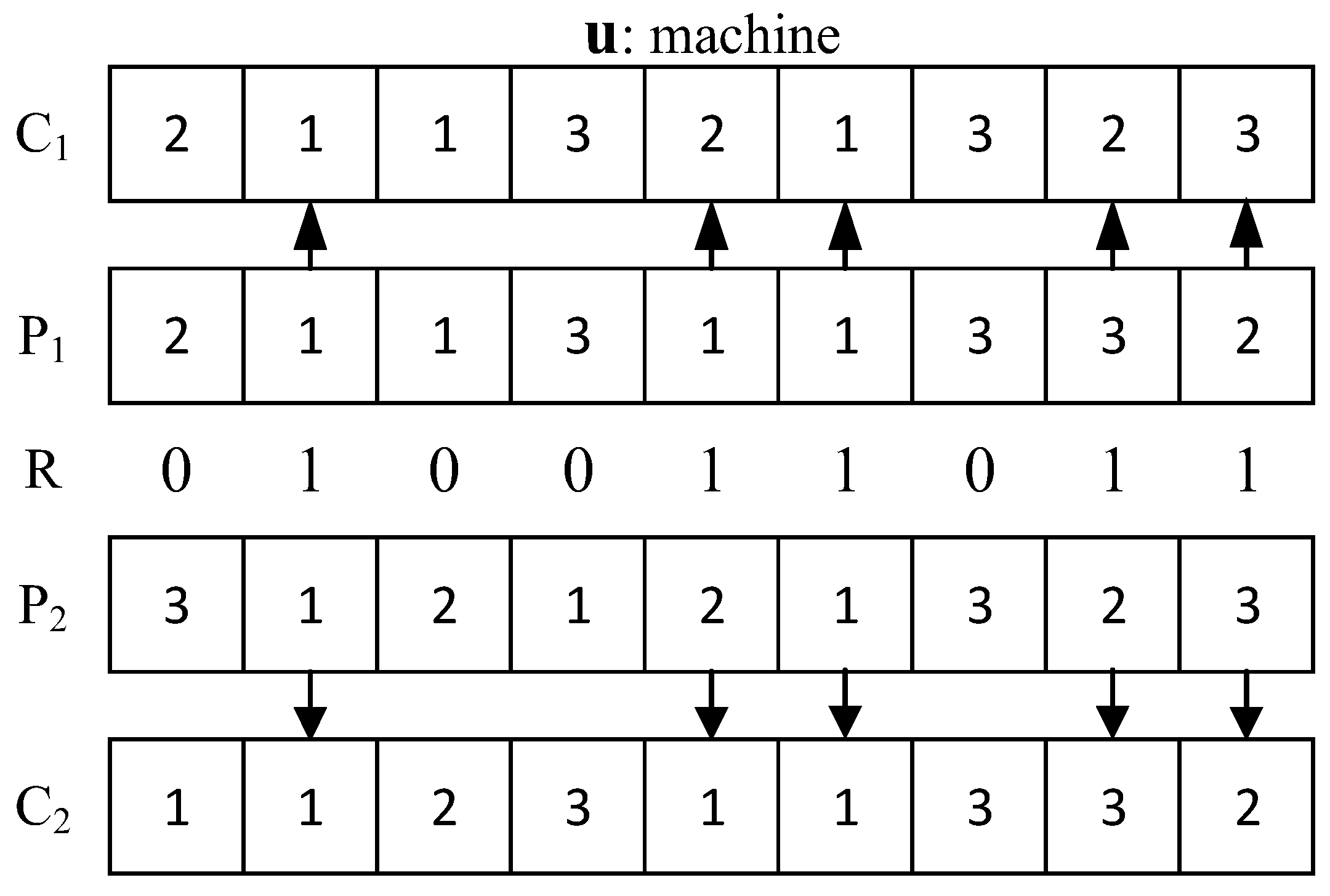
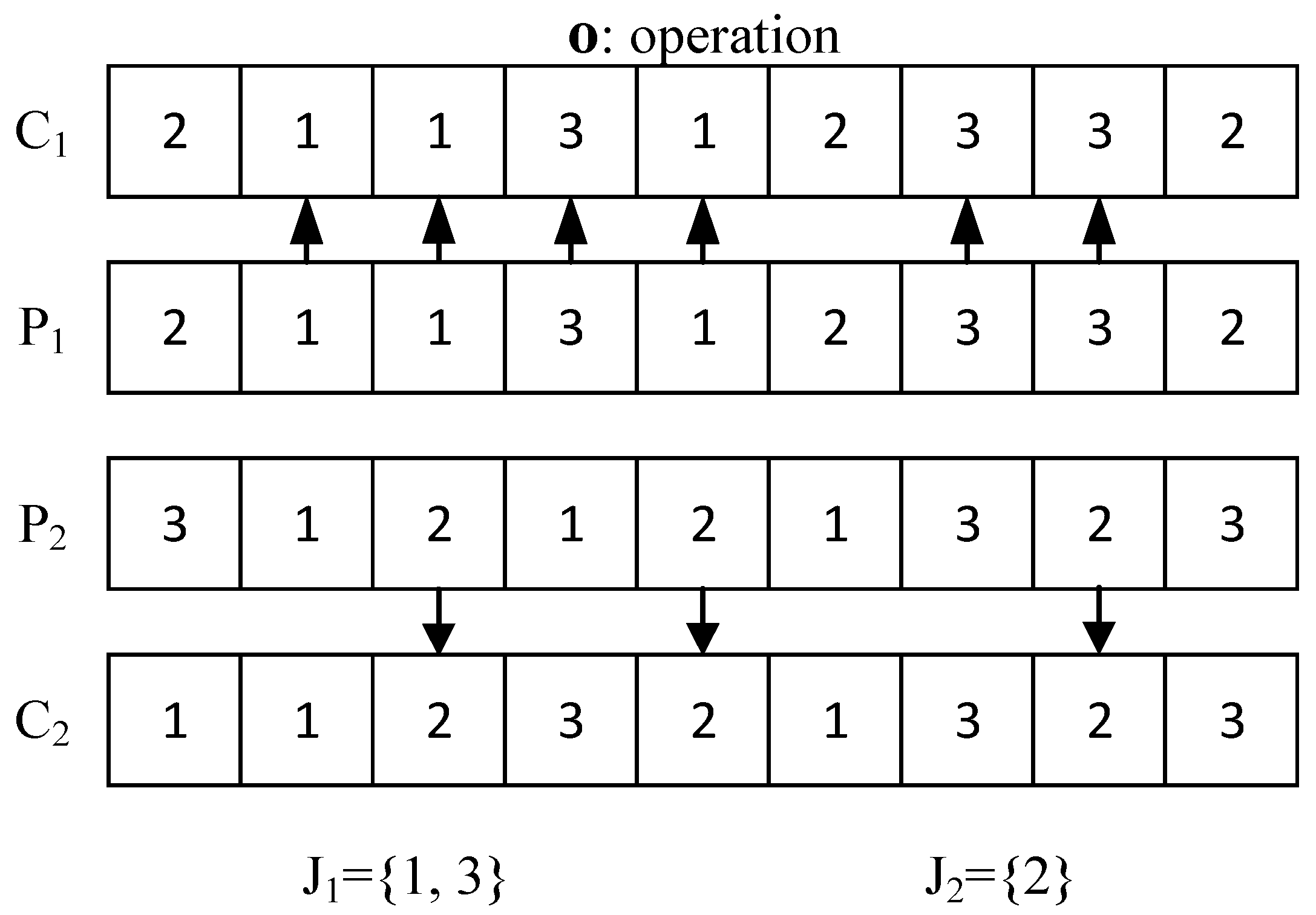
3.1.5. Search Operator

Two kinds of search operators (i.e., POX and MPX) are used in this article. In detail, the operation-based crossover (POX) operator is applied for the operation part o . Multiple point crossover (MPX) is conducted in the machine assignment part u . Figure 3 gives an illustration of the POX operator. The main procedures of POX are stated below.
Step 1: For one solution, all operations in the first part o are grouped into two sets, which are denoted by symbols J1 and J2.
Step 2: Jobs included in J1 from P1 to child one (denoted by C1) are copied, and jobs included in J2 from P2 to child two (denoted by C2) are copied. Meanwhile, their order is kept unchanged in the offspring.
Step 3: Jobs included in J2 from P2 to C1 and jobs included in J1 from P1 to C2 are copied. Their order is kept unchanged in the offspring.
Figure 4 illustrates the search process of the MPX operator. The main steps of MPX are presented below.
Step 1: Randomly generate a set (denoted by R) consisting of 0–1 binary values, and the length of this set is equal to the length of an operation list.
Step 2: Select operations from P1 and P2 where the corresponding value is equal to the one in R. Then, swap their corresponding machines. The other machines in P1 and P2 are reserved for the offspring.
The main procedures of the mutation operator are detailed below.
Step 1: Randomly select two locations in the first part and swap two corresponding elements between two positions.
Step 2: Randomly select one machine from the available machines in the corresponding positions.
Step 3: Adjust processing time in a feasible range for the corresponding positions.

3.1.6. Local Search

In shop scheduling problems, variable neighborhood search (VNS) is an essential local search strategy [32,33]. VNS can search for promising solutions by using a variety of neighborhood search structures. The inner loop of VNS often comprises shake and local search operators. To improve the search diversity, shake operation can change from one type of local search neighborhood to another. To enhance the quality of solutions, the local search operator searches for high-quality solutions in the vicinity of solutions. Please refer to [10] for detailed information. Furthermore, the number of VNS structures is fixed to reduce computation time. In this paper, three types of VNS are employed, which are elucidated as follows:
(1)
Insert operator: Two different positions on the first part of one solution are chosen at random, and then the operation in the latter position is inserted into the former position.
(2)
Swap operator: Two different positions on the first part of one solution are chosen at random and the two corresponding operations are exchanged.
(3)
Reverse operator: Two different positions on the first part of one solution are chosen at random and a set of operations between two positions are reversed.
The detailed procedure of VNS in this work is as follows: First of all, one candidate solution is picked from one population. Then, one new solution would be yielded by utilizing one of three types of neighborhood structures. If the newly yielded solution is superior to the original one based on fitness, the new solution will replace the old one and continue the inner loop. If the local search rule reaches Ls times and the new solution is not improved, this local search will be terminated.

4. Numerical Experiments

This part is committed to measuring the behavior of MOCMOA. At first, the instances and parameter calibration are discussed. Then, three metrics are stated. Finally, comparison experiments are presented in this part. All the trials were carried out on a PC with an Intel Core i7, 2.70 GHz, 16 GB of RAM, and Win 10. Additionally, all experiments were implemented by java.

4.1. Instances and Metrics

To systematically evaluate the performance of approaches, test instances and metrics are adopted in this part. Because energy-efficient FJSP-CPT is a new combinatorial optimization problem, we modified instances based on classical benchmarks MK01~MK15. That is to say, the original data remained unchanged and the other related data of these instances are recorded in Table 1.
In this work, three common metrics, including Spread, GD [34], and IGD [35], were utilized to measure the performance of one certain algorithm. A normalization approach was adopted in these metrics. These metrics are defined in the following part.
(1)
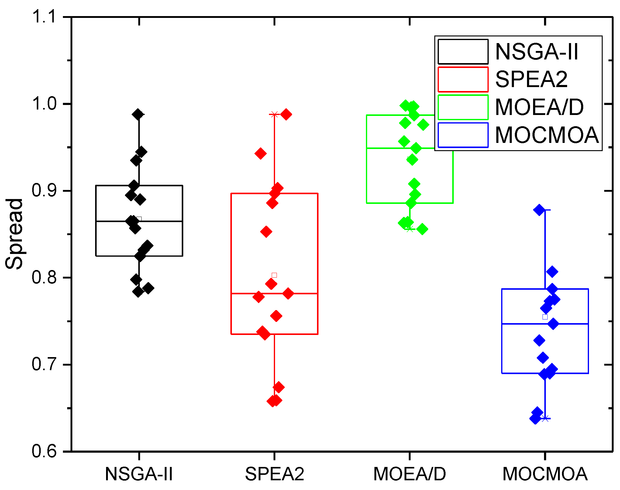
Spread (Δ). It is a measure of solution distribution. It is capable of determining the distribution situation along the front. This metric’s definition is as follows [36]:
= j = 1 n o d j e + i = 1 | PF | | d i d ¯ | j = 1 n o d j e + | PF | · d ¯
where d i is Euclidean distance from the i-th member in PF to its closest one, d ¯ is the average distance among all d i , d j e is the Euclidean distance from the j-th objective to the boundary value in the PF*, | PF | is the total number of PF points, and one smaller Spread value is desirable.
(2)
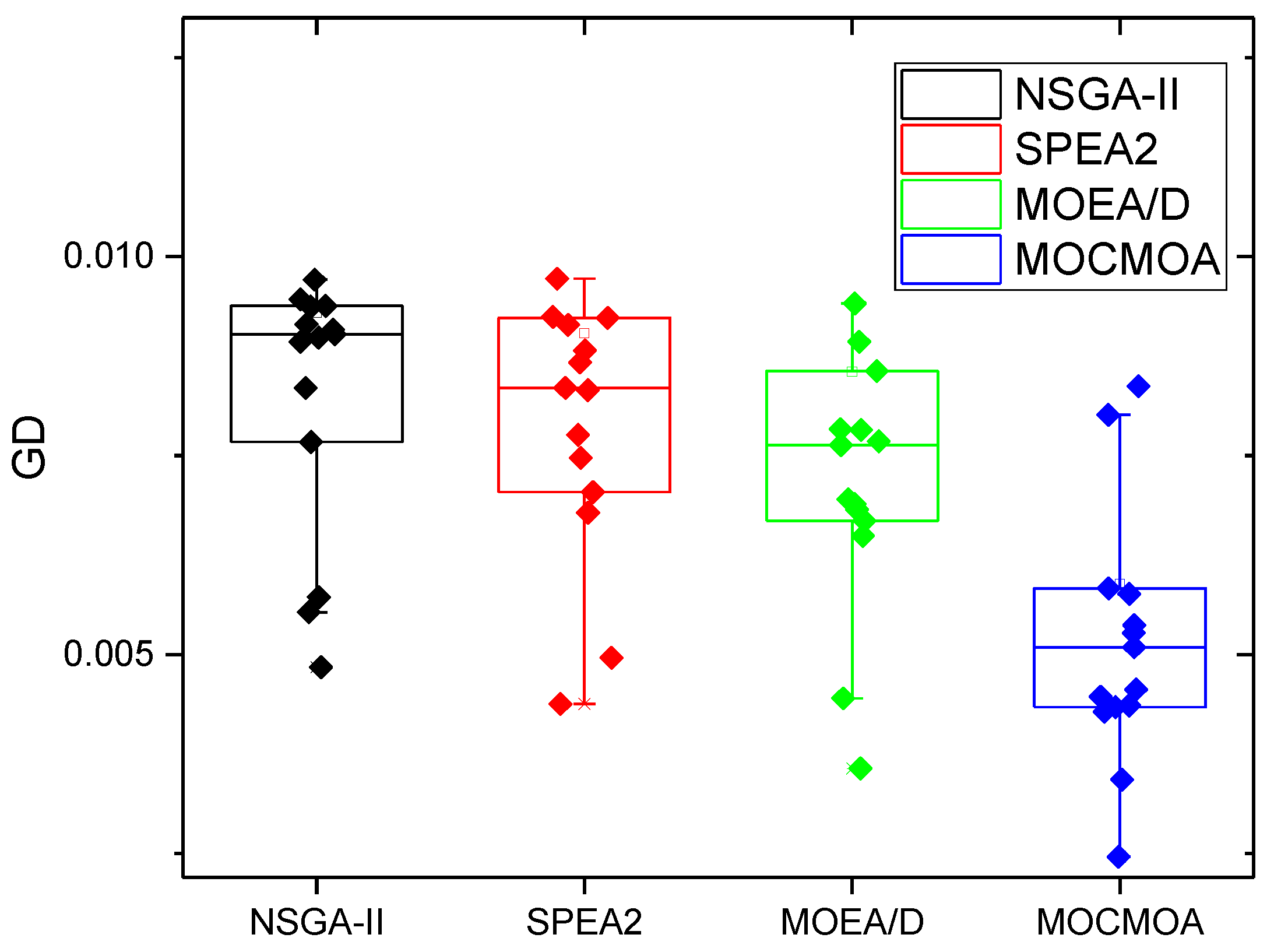
Generational Distance (GD). The convergence performance is represented by the GD measure. Its average gap is between PF and PF*. The formula for this metric is as follows:
GD = i = 1 | PF | D i 2 | PF |
where D i is the Euclidean distance from the i-th member in PF to the closest one in PF*, and one smaller GD value is desirable.
(3)
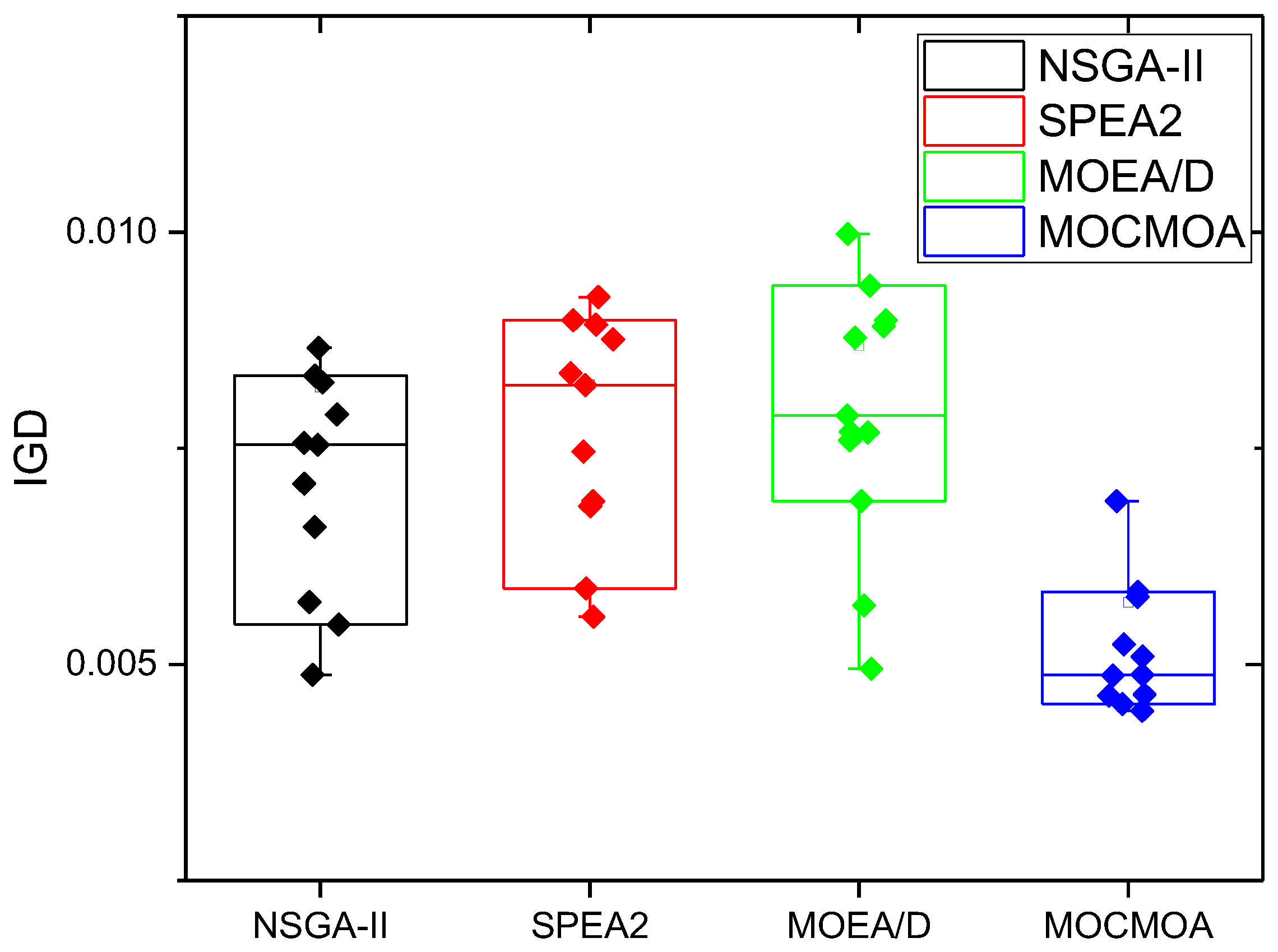
Inverted Generational Distance (IGD). It is a different version of the GD; however, it is a more thorough indicator. It determines the average distance between PF* and PF. The following is a definition of IGD:
IGD = x PF d i s t ( x , PF ) | PF |
where d i s t ( x , PF ) is the minimum Euclidean distance from the x ( x is the member in PF*) to the member in PF, | PF | is the total number of all PF* points. A smaller IGD value is good.

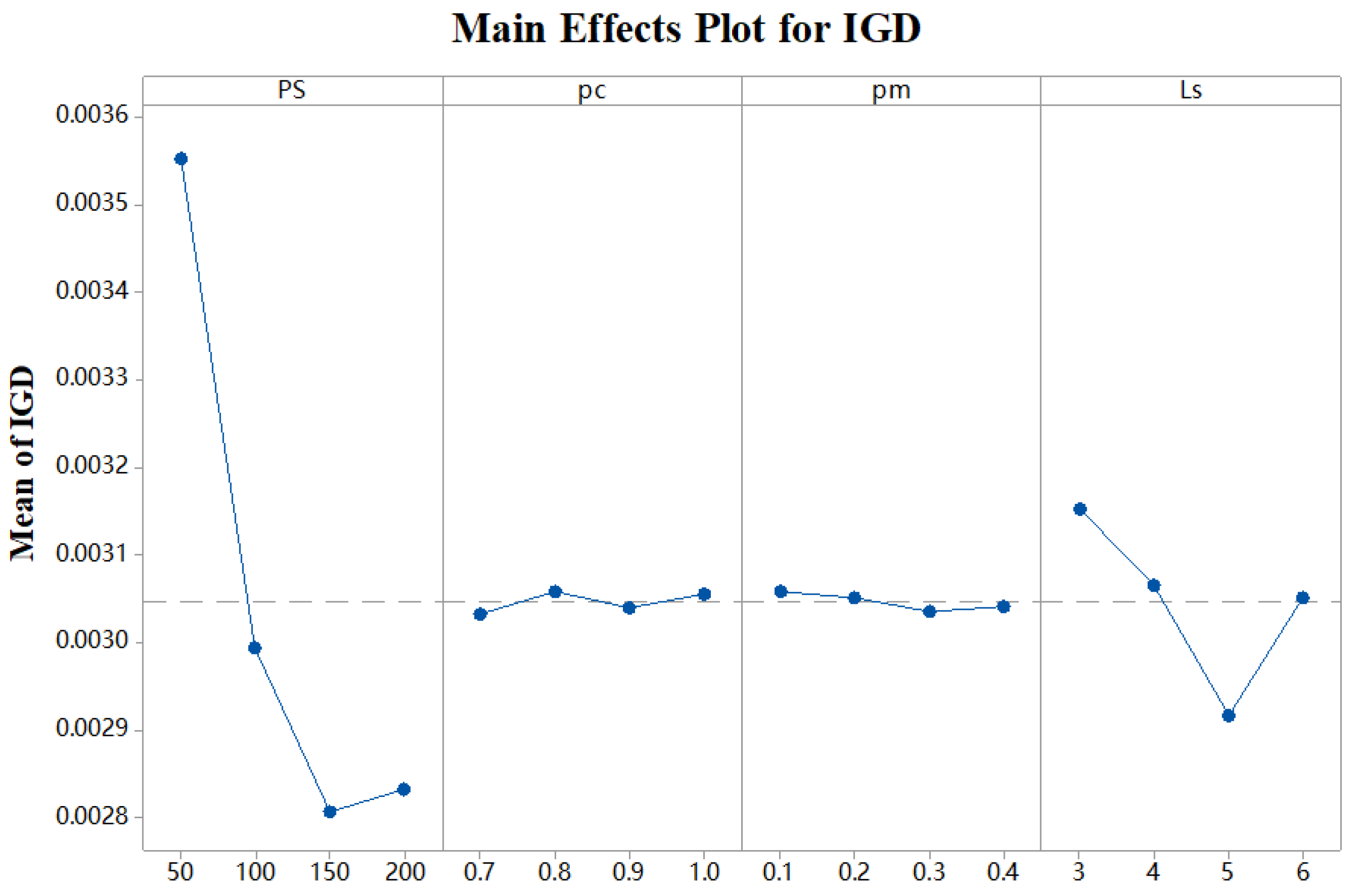
4.2. Parameter Calibration

The behavior of algorithms depends on parameter settings. Thus, some experiments were performed to assess various parameter combinations of MOCMOA. MOCMOA includes four parameters: population size (PS), crossover ratio (pc), mutation ratio (pm), and times of local search (Ls). A Taguchi approach was utilized to determine the optimal parameter combination in all instances. Levels of these parameters in MOCMOA are defined: P S = { 50 , 100 , 150 , 200 } , p c = { 0.7 , 0.8 , 0.9 , 1.0 } , p m = { 0.1 , 0.2 , 0.3 , 0.4 } , and Ls = { 3 , 4 , 5 , 6 } . Consequently, one orthogonal array L16 (44) was employed in this trial. All experiments were carried out with 20 runs regarding each parameter combination. Figure 5 presents the main effect graph of these parameters in terms of IGD metric. As mentioned earlier, one smaller IGD value is desirable. According to the observation in Figure 5, the optimal parameter combination of MOCMOA is: PS = 150, p c = 0.9, p m = 0.3, and Ls = 5.

4.3. Comparison Experiment

To measure the comprehensive behavior of the MOCMOA approach, MOCMOA was compared against some famous multi-objective evolutionary algorithms (MOEAs) such as NSGA-II [37], SPEA2 [35], and MOEA/D [38]. As mentioned earlier, energy-efficient FJSP-CPT has not yet been solved by any optimization algorithm, because it is a new shop scheduling problem. To this end, these compared MOEAs should be modified to meet the characteristics of energy-efficient FJSP-CPT. These compared algorithms’ parameters were calibrated in the same way as the previous experiment. The comparison experiment is performed in this section. For a fair comparison, all the algorithms considered in this comparison experiment adopted the same terminal condition, namely, the maximum number of function evaluations (MNFEs). When the terminal condition (i.e., MNFEs) is met, the approach will stop the loop. The MNFEs is usually related to the problem scale. Therefore, MNFEs is equal to 45,000.
Because of the stochastic characteristic of metaheuristics, each method carried out 30 repetitions for each test instance to reduce randomness. Furthermore, a significant test was employed in the results among different algorithms. In this paper, at the 0.95 significance level, a Friedman test was adopted to assess the significant difference in terms of statistical results by all algorithms.
Table 2 records the numerical values (i.e., mean and standard deviation) in terms of the GD metric. The best value is identified in bold. As shown in Table 2, the statistical values of the proposed MOCMOA are smaller than those of other MOEAs in all instances. It indicates that the MOCMOA algorithm outperforms its competitors. Table 3 shows the ranks among these algorithms in all instances by using the Friedman test regarding the GD metric. These statistical results further confirm that MOCMOA is the best one among all algorithms regarding the GD metric. Similarly, it can be seen from Table 4 that the MOCMOA can obtain better results regarding the Spread metric. To be specific, MOCMOA finds the best mean values in 14 out of 15 instances, except for “MK06”. Furthermore, MOCMOA can achieve the best standard deviation values in 14 out of 15 instances, which implies the good stability of the proposal. Meanwhile, as shown in Table 5, MOCMOA is superior to its competitors in most instances concerning the Spread metric by a large margin. Table 6 and Table 7 show the statistical results obtained by these MOEAs regarding the IGD metric. As presented in Table 6, it can be seen that the MOCMOA can find the best mean standard deviation IGD values among these algorithms. Table 7 records all ranks of algorithms by using the Friedman test regarding the IGD metric. Apparently, the MOCMOA shows good behavior regarding convergence and diversity performance. Numerical results confirm that the proposed MOCMOA is capable of addressing such a combinatorial optimization issue well.
To further visualize the behavior of various optimization algorithms, Figure 6, Figure 7 and Figure 8 plot the distribution of three metrics obtained by these algorithms on all problems. Figure 6 presents the distribution of statistical results regarding the GD metric for four algorithms in 20 independent run times. As shown in Figure 6, the average results found by the MOCMOA are lower than those by its compared approaches with respect to the convergence performance. Furthermore, there is no overlap among different algorithms. This plot further verifies our conclusion from the previous numerical experiment. As shown in Figure 7, the average results found by the MOCMOA are lower than those by its competitors regarding the diversity of solutions. As shown in Figure 8, regarding the comprehensive performance, the average results found by the MOCMOA are lower than those by its competitors by a large margin. Meanwhile, there is no overlap among these algorithms. Therefore, it is concluded that the MOCMOA is significantly better than the other rivals for energy-efficient FJSP-CPT. The good performance of MOCMOA is attributed to the fact that it combines the advantages of cellular structure for exploration and VNS for exploitation. In this algorithm, cellular structure is utilized to enhance the search performance. Meanwhile, we utilize VNS as a general local search to further improve the quality of solution. The advantages of the proposed MOCMOA are the good convergence and diversity performance. However, the disadvantages of the MOCMOA lie in consuming a lot of time searching for good solutions.

5. Conclusions and Outlook

In this work, an energy-efficient flexible job shop scheduling problem with controllable processing times (FJSP-CPT) was investigated. This work was an important supplement to the present studies where most existing research ignored green-related criteria. In addition to the common makespan criterion, total energy consumption (TEC) was regarded as a new green criterion. Consequently, a mathematical model of the green FJSP-CPT with objectives of minimization TEC and makespan was formulated in this paper. For this purpose, a multi-objective cellular memetic optimization algorithm (MOCMOA) was designed to handle this optimization problem. This MOCMOA combined the advantages of cellular structure and variable neighborhood search, allowing for a suitable balance of global exploitation and local exploration. To prove the validity of the proposed MOCMOA, comparison experiments on some instances were made. Experimental results revealed that MOCMOA was a promising approach to solve such a problem compared to other algorithms.
In future work, more complex shop scheduling problems, including a dynamic scheduling environment and distributed shop scheduling environment, will be explored. Furthermore, more effective optimization metaheuristics and heuristics are proposed to address such scheduling problems.

Author Contributions

Y.W.: Conceptualization, Methodology, Software. W.P.: Data curation, Writing—Original draft preparation. C.L.: Supervision. H.X.:Writing—Reviewing and Editing. All authors have read and agreed to the published version of the manuscript.

Funding

This work was supported by National Natural Science Foundation of China under Grant no. 52175490 and 51805495.

Data Availability Statement

Data available on request from the authors.

Conflicts of Interest

The authors declare no conflict of interest.

Nomenclature

(1) Parameters
total number of jobs
m total number of machines.
k index   of   machines ,   k = 1 , 2 , , m .
i , g index   of   jobs ,   i . e . ,   i , g = 1 , 2 , .. , n .
j , h index   of   operations ,   j , h = 1 , 2 , , n j .
O ij the   j - th   operation   of   job   i .
n i total   number   of   operations   of   job   i .
C ijk the   completion   time   of   O i j   on   machine   k .
S ijk the   starting   time   of   O i j   on   machine   k .
p ijk L the   lowest   value   of   processing   time   of   O ij   on   machine   k .
p ijk U the   upper   value   of   processing   time   of   O ij   on   machine   k .
ij available   machine   set   for   O ij .
C max the makespan of the schedule.
P k idle the   idle   power   of   a   machine   k .
P k work the   work   power   of   a   machine   k .
EC w the energy consumption during the work phase.
EC s the energy consumption during the idle phase.
L one very large number.
(2) Decision variables
p ijk a the   actual   processing   time   of   O i j on machine k
X i j k = { 1 ,   if   the   operation   O i j   is   processed   on   machine   k 0 ,   elsewise  
Y g h i j k = { 1 ,   if   O g h   is   the   predecessor   of   O i j   on   machine   k 0 ,   elsewise  

References

  1. Lu, C.; Huang, Y.; Meng, L.; Gao, L.; Zhang, B.; Zhou, J. A Pareto-based collaborative multi-objective optimization algorithm for energy-efficient scheduling of distributed permutation flow-shop with limited buffers. Robot. Comput. Manuf. 2022, 74, 102277. [Google Scholar] [CrossRef]
  2. Lu, C.; Zhang, B.; Gao, L.; Yi, J.; Mou, J. A Knowledge-Based Multiobjective Memetic Algorithm for Green Job Shop Scheduling With Variable Machining Speeds. IEEE Syst. J. 2022, 16, 844–855. [Google Scholar] [CrossRef]
  3. Jia, J.; Lu, C.; Yin, L. Energy Saving in Single-Machine Scheduling Management: An Improved Multi-Objective Model Based on Discrete Artificial Bee Colony Algorithm. Symmetry 2022, 14, 561. [Google Scholar] [CrossRef]
  4. Gahm, C.; Denz, F.; Dirr, M.; Tuma, A. Energy-efficient scheduling in manufacturing companies: A review and research framework. Eur. J. Oper. Res. 2016, 248, 744–757. [Google Scholar] [CrossRef]
  5. Gao, K.; Huang, Y.; Sadollah, A.; Wang, L. A review of energy-efficient scheduling in intelligent production systems. Complex Intell. Syst. 2020, 6, 237–249. [Google Scholar] [CrossRef] [Green Version]
  6. Mansouri, S.A.; Aktas, E.; Besikci, U. Green scheduling of a two-machine flowshop: Trade-off between makespan and energy consumption. Eur. J. Oper. Res. 2016, 248, 772–788. [Google Scholar] [CrossRef] [Green Version]
  7. Liu, Z.; Yan, J.; Cheng, Q.; Yang, C.; Sun, S.; Xue, D. The mixed production mode considering continuous and intermittent processing for an energy-efficient hybrid flow shop scheduling. J. Clean. Prod. 2020, 246, 119071. [Google Scholar] [CrossRef]
  8. Lu, C.; Gao, L.; Li, X.; Pan, Q.-K.; Wang, Q. Energy-efficient permutation flow shop scheduling problem using a hybrid multi-objective backtracking search algorithm. J. Clean. Prod. 2017, 144, 228–238. [Google Scholar] [CrossRef]
  9. Li, J.-Q.; Sang, H.-Y.; Han, Y.-Y.; Wang, C.-G.; Gao, K.-Z. Efficient multi-objective optimization algorithm for hybrid flow shop scheduling problems with setup energy consumptions. J. Clean. Prod. 2018, 181, 584–598. [Google Scholar] [CrossRef]
  10. Lu, C.; Gao, L.; Pan, Q.-K.; Li, X.; Zheng, J. A multi-objective cellular grey wolf optimizer for hybrid flowshop scheduling problem considering noise pollution. Appl. Soft Comput. 2019, 75, 728–749. [Google Scholar] [CrossRef]
  11. Li, M.; Lei, D.; Cai, J. Two-level imperialist competitive algorithm for energy-efficient hybrid flow shop scheduling problem with relative importance of objectives. Swarm Evol. Comput. 2019, 49, 34–43. [Google Scholar] [CrossRef]
  12. Zuo, Y.; Fan, Z.; Zou, T.; Wang, P. A Novel Multi-Population Artificial Bee Colony Algorithm for Energy-Efficient Hybrid Flow Shop Scheduling Problem. Symmetry 2021, 13, 2421. [Google Scholar] [CrossRef]
  13. Wang, S.; Wang, X.; Chu, F.; Yu, J. An energy-efficient two-stage hybrid flow shop scheduling problem in a glass production. Int. J. Prod. Res. 2020, 58, 2283–2314. [Google Scholar] [CrossRef]
  14. Lei, D.; Gao, L.; Zheng, Y. A novel teaching-learning-based optimization algorithm for energy-efficient scheduling in hybrid flow shop. IEEE Trans. Eng. Manag. 2018, 65, 330–340. [Google Scholar] [CrossRef]
  15. Gong, G.; Chiong, R.; Deng, Q.; Han, W.; Zhang, L.; Lin, W.; Li, K. Energy-efficient flexible flow shop scheduling with worker flexibility. Expert Syst. Appl. 2020, 141, 112902. [Google Scholar] [CrossRef]
  16. Zhang, B.; Pan, Q.-K.; Gao, L.; Meng, L.-L.; Li, X.-Y.; Peng, K.-K. A Three-Stage Multiobjective Approach Based on Decomposition for an Energy-Efficient Hybrid Flow Shop Scheduling Problem. IEEE Trans. Syst. Man Cybern. Syst. 2020, 50, 4984–4999. [Google Scholar] [CrossRef]
  17. May, G.; Stahl, B.; Taisch, M.; Prabhu, V. Multi-objective genetic algorithm for energy-efficient job shop scheduling. Int. J. Prod. Res. 2015, 53, 7071–7089. [Google Scholar] [CrossRef]
  18. Zhang, R.; Chiong, R. Solving the energy-efficient job shop scheduling problem: A multi-objective genetic algorithm with enhanced local search for minimizing the total weighted tardiness and total energy consumption. J. Clean. Prod. 2016, 112, 3361–3375. [Google Scholar] [CrossRef]
  19. Yin, L.; Li, X.; Gao, L.; Lu, C.; Zhang, Z. Energy-efficient job shop scheduling problem with variable spindle speed using a novel multi-objective algorithm. Adv. Mech. Eng. 2017, 9, 1687814017695959. [Google Scholar] [CrossRef] [Green Version]
  20. Giglio, D.; Paolucci, M.; Roshani, A. Integrated lot sizing and energy-efficient job shop scheduling problem in manufacturing/remanufacturing systems. J. Clean. Prod. 2017, 148, 624–641. [Google Scholar] [CrossRef]
  21. He, L.; Chiong, R.; Li, W.; Dhakal, S.; Cao, Y.; Zhang, Y. Multiobjective Optimization of Energy-Efficient JOB-Shop Scheduling with Dynamic Reference Point-Based Fuzzy Relative Entropy. IEEE Trans. Ind. Inform. 2022, 18, 600–610. [Google Scholar] [CrossRef]
  22. Abedi, M.; Chiong, R.; Noman, N.; Zhang, R. A multi-population, multi-objective memetic algorithm for energy-efficient job-shop scheduling with deteriorating machines. Expert Syst. Appl. 2020, 157, 113348. [Google Scholar] [CrossRef]
  23. Yin, L.; Li, X.; Gao, L.; Lu, C.; Zhang, Z. A novel mathematical model and multi-objective method for the low-carbon flexible job shop scheduling problem. Sustain. Comput. Inform. Syst. 2017, 13, 15–30. [Google Scholar] [CrossRef]
  24. Zhang, L.; Tang, Q.; Wu, Z.; Wang, F. Mathematical modeling and evolutionary generation of rule sets for energy-efficient flexible job shops. Energy 2017, 138, 210–227. [Google Scholar] [CrossRef]
  25. Luo, S.; Zhang, L.; Fan, Y. Energy-efficient scheduling for multi-objective flexible job shops with variable processing speeds by grey wolf optimization. J. Clean. Prod. 2019, 234, 1365–1384. [Google Scholar] [CrossRef]
  26. Duan, J.; Wang, J. Energy-efficient scheduling for a flexible job shop with machine breakdowns considering machine idle time arrangement and machine speed level selection. Comput. Ind. Eng. 2021, 161, 107677. [Google Scholar] [CrossRef]
  27. Li, M.; Lei, D. An imperialist competitive algorithm with feedback for energy-efficient flexible job shop scheduling with transportation and sequence-dependent setup times. Eng. Appl. Artif. Intell. 2021, 103, 104307. [Google Scholar] [CrossRef]
  28. Lu, C.; Li, X.; Gao, L.; Liao, W.; Yi, J. An effective multi-objective discrete virus optimization algorithm for flexible job-shop scheduling problem with controllable processing times. Comput. Ind. Eng. 2017, 104, 156–174. [Google Scholar] [CrossRef]
  29. Lu, C.; Gao, L.; Gong, W.; Hu, C.; Yan, X.; Li, X. Sustainable scheduling of distributed permutation flow-shop with non-identical factory using a knowledge-based multi-objective memetic optimization algorithm. Swarm Evol. Comput. 2021, 60, 100803. [Google Scholar] [CrossRef]
  30. Lu, C.; Gao, L.; Yi, J. Grey wolf optimizer with cellular topological structure. Expert Syst. Appl. 2018, 107, 89–114. [Google Scholar] [CrossRef]
  31. Golchin, M.; Liew, A.W.C. Parallel biclustering detection using strength Pareto front evolutionary algorithm. Inf. Sci. 2017, 415, 283–297. [Google Scholar] [CrossRef]
  32. Mladenovic, N.; Hansen, P. Variable neighborhood search. Comput. Oper. Res. 1997, 24, 1097–1100. [Google Scholar] [CrossRef]
  33. Lu, C.; Gao, L.; Yi, J.; Li, X. Energy-Efficient Scheduling of Distributed Flow Shop with Heterogeneous Factories: A Real-World Case From Automobile Industry in China. IEEE Trans. Ind. Inform. 2020, 17, 6687–6696. [Google Scholar] [CrossRef]
  34. Zitzler, E.; Deb, K.; Thiele, L. Comparison of Multiobjective Evolutionary Algorithms: Empirical Results. Evol. Comput. 2000, 8, 173–195. [Google Scholar] [CrossRef] [PubMed] [Green Version]
  35. Zitzler, E.; Thiele, L. Multiobjective evolutionary algorithms: A comparative case study and the Strength Pareto approach. IEEE Trans. Evol. Comput. 1999, 3, 257–271. [Google Scholar] [CrossRef] [Green Version]
  36. Shen, X.-N.; Yao, X. Mathematical modeling and multi-objective evolutionary algorithms applied to dynamic flexible job shop scheduling problems. Inf. Sci. 2015, 298, 198–224. [Google Scholar] [CrossRef] [Green Version]
  37. Deb, K.; Pratap, A.; Agarwal, S.; Meyarivan, T. A fast and elitist multiobjective genetic algorithm: NSGA-II. IEEE Trans. Evol. Comput. 2002, 6, 182–197. [Google Scholar] [CrossRef] [Green Version]
  38. Li, H.; Zhang, Q. Multiobjective Optimization Problems with Complicated Pareto Sets, MOEA/D and NSGA-II. IEEE Trans. Evol. Comput. 2009, 13, 284–302. [Google Scholar] [CrossRef]
Figure 1. Flowchart of the proposed MOCMOA.
Symmetry 14 00832 g001
Figure 2. Solution representation.
Symmetry 14 00832 g002
Figure 3. POX operator.
Symmetry 14 00832 g003
Figure 4. MPX operator.
Symmetry 14 00832 g004
Figure 5. Main effect graph of four parameters.
Symmetry 14 00832 g005
Figure 6. Solution distributions among four algorithms in terms of GD.
Symmetry 14 00832 g006
Figure 7. Solution distributions among four algorithms in terms of Spread.
Symmetry 14 00832 g007
Figure 8. Solution distributions among four algorithms in terms of IGD.
Symmetry 14 00832 g008
Table 1. Data of instances.
ParameterDistribution
minimization   processing   time   ( p ijk L ) 30 min
maximization   processing   time   ( p ijk U ) 50 min
idle   power   on   each   machine   k   ( P k idle ) continuous uniform (0, 2] kW
work   power   on   each   machine   k   ( P k work ) continuous uniform [2, 5] kW
Table 2. Mean and standard deviation of GD among all algorithms.
InstancesNSGA-II
(Mean/Standard Deviation)
SPEA2
(Mean/Standard Deviation)
MOEA/D
(Mean/Standard Deviation)
MOCMOA
(Mean/Standard Deviation)
MK015.72 × 10−3/3.3 × 10−34.38 × 10−3/3.6 × 10−34.45 × 10−3/4.2 ×10−32.46 × 10−3/1.3 × 10−3
MK024.84 × 10−3/4.3 × 10−34.96 × 10−3/4.7 × 10−33.57 × 10−3/5.5 ×10−33.43 × 10−3/1.6 × 10−3
MK035.53 × 10−3/2.8 × 10−36.78 × 10−3/3.5 × 10−36.68 × 10−3/3.2 ×10−34.47 × 10−3/2.1 × 10−3
MK047.67 × 10−3/2.6 × 10−38.35 × 10−3/2.8 × 10−37.82 × 10−3/3.7 ×10−35.27 × 10−3/2.6 × 10−3
MK058.35 × 10−3/2.1 × 10−37.47 × 10−3/2.6 × 10−36.95 × 10−3/2.9 ×10−34.28 × 10−3/1.7 × 10−3
MK062.4 × 10−2/1.9 × 10−22.56 × 10−2/1.9 × 10−22.86 × 10−2/2.0 × 10−21.67 ×10−2/1.6 ×10−2
MK079.46 × 10−3/1.9 × 10−38.67 × 10−3/1.8 × 10−37.68 × 10−3/1.8 × 10−35.83 × 10−3/1.1 × 10−3
MK089.37 × 10−3/2.7 × 10−37.76 × 10−3/1.9 × 10−36.89 × 10−3/2.5 × 10−34.36 × 10−3/1.1 × 10−3
MK098.93 × 10−3/2.3 × 10−38.82 × 10−3/2.1 × 10−36.49 × 10−3/2.4 × 10−35.09 × 10−3/1.8 × 10−3
MK109.02 × 10−3/2.1 × 10−38.32 × 10−3/2.2 × 10−36.82 × 10−3/2.1 × 10−34.56 × 10−3/1.6 × 10−3
MK119.71 × 10−3/2.7 × 10−37.04 × 10−3/1.9 × 10−37.83 × 10−3/1.9 × 10−34.34 × 10−3/1.2 × 10−3
MK129.38 × 10−3/3.2 × 10−39.24 × 10−3/3.1 × 10−39.41 × 10−3/2.2 × 10−38.37 × 10−3/2.1 × 10−3
MK138.98 × 10−3/2.8 × 10−39.14 × 10−3/2.7 × 10−37.63 × 10−3/2.9 × 10−35.76 × 10−3/2.2 × 10−3
MK149.08 × 10−3/2.5 × 10−39.23 × 10−3/2.6 × 10−38.56 × 10−3/2.7 × 10−35.37 × 10−31.9 × 10⁻³
MK159.15 × 10−3/4.6 × 10−39.72 × 10−3/4.2 × 10−38.93 × 10−3/3.7 × 10−38.01 × 10−3/2.8 × 10−3
Table 3. Ranks among algorithms using the Friedman test regarding the GD metric.
MOEAsRankp-Value
NSGA-II4.001.35 × 10−9
SPEA23.05
MOEA/D2.85
MOCMOA1.00
Table 4. Mean and standard deviation of Spread among all algorithms.
InstancesNSGA-II
(Mean/Standard Deviation)
SPEA2
(Mean/Standard Deviation)
MOEA/D
(Mean/Standard Deviation)
MOCMOA (Mean/Standard Deviation)
MK018.90 × 10−1/4.5 × 10−27.38 × 10−1/3.7 × 10−29.78 × 10−1/4.9 × 10−26.89 × 10−1/3.5 × 10−2
MK029.45 × 10−1/4.4 × 10−27.82 × 10−1/3.5 × 10−29.87 × 10−1/4.3 × 10−27.65 × 10−1/3.0 × 10−2
MK038.57 × 10−1/5.2 × 10−26.59 × 10−1/4.9 × 10−29.49 × 10−1/5.3 × 10−26.38 × 10−1/3.6 × 10−2
MK049.35 × 10−1/5.9 × 10−27.35 × 10−1/4.8 × 10−29.08 × 10−1/5.7 × 10−26.95 × 10−1/4.2 × 10−2
MK058.65 × 10−1/4.3 × 10−26.58 × 10−1/4.6 × 10−28.64 × 10−1/6.2 × 10−26.45 × 10−1/4.1 × 10−2
MK069.88 × 10−1/5.8 × 10−29.03 × 10−1/4.1 × 10−29.98 × 10−1/6.8 × 10−29.97 × 10−1/6.4 × 10−2
MK078.65 × 10−1/6.3 × 10−28.86 × 10−1/5.8 × 10−29.76 × 10−1/5.8 × 10−27.28 × 10−1/3.9 × 10−2
MK087.98 × 10−1/4.8 × 10−27.93 × 10−1/5.8 × 10−28.86 × 10−1/6.8 × 10−26.90 × 10−1/3.8 × 10−2
MK098.95 × 10−1/6.3 × 10−28.97 × 10−1/7.2 × 10−28.96 × 10−1/5.6 × 10−27.87 × 10−1/4.9 × 10−2
MK107.88 × 10−1/4.4 × 10−27.56 × 10−1/5.5 × 10−29.36 × 10−1/4.6 × 10−27.47 × 10−1/4.2 × 10−2
MK117.84 × 10−1/5.6 × 10−26.74 × 10−1/5.9 × 10−28.63 × 10−1/7.1 × 10−27.08 × 10−1/4.7 × 10−2
MK128.32 × 10−1/5.7 × 10−27.78 × 10−1/5.5 × 10−29.96 × 10−1/6.6 × 10−27.75 × 10−1/4.8 × 10−2
MK138.25 × 10−1/6.3 × 10−28.53 × 10−1/6.5 × 10−29.57 × 10−1/7.3 × 10−27.73 × 10−1/4.8 × 10−2
MK148.37 × 10−1/6.2 × 10−29.88 × 10−1/5.9 × 10−28.56 × 10−1/6.9 × 10−28.07 × 10−1/5.5 × 10−2
MK159.06 × 10−1/6.5 × 10−29.43 × 10−1/6.5 × 10−29.97 × 10−1/8.3 × 10−28.78 × 10−1/6.1 × 10−2
Table 5. Ranks among algorithms using the Friedman test regarding the Spread metric.
MOEAsRankp-Value
NSGA-II2.864.95 × 10−5
SPEA22.05
MOEA/D4.00
MOCMOA1.45
Table 6. Mean and standard deviation of IGD metric among all algorithms.
InstancesNSGA-II
(Mean/Standard Deviation)
SPEA2
(Mean/Standard Deviation)
MOEA/D
(Mean/Standard Deviation)
MOCMOA (Mean/Standard Deviation)
MK015.56 × 10−4/6.6 × 10−54.98 × 10−4/6.7 × 10−57.59 × 10−3/6.8 × 10−54.42 × 10−4/5.3 × 10−5
MK024.76 × 10−4/6.3 × 10−54.87 × 10−4/6.6 × 10−56.93 × 10−4/8.2 × 10−54.37 × 10−4/5.8 × 10−5
MK034.88 × 10−3/2.2 × 10−35.55 × 10−3/2.4 × 10−34.95 × 10−3/4.5 × 10−34.64 × 10−3/1.6 × 10−3
MK048.34 × 10−3/2.6 × 10−38.37 × 10−3/2.7 × 10−37.68 × 10−3/3.1 × 10−35.46 × 10−3/1.8 × 10−3
MK055.72 × 10−3/6.7 × 10−45.88 × 10−3/7.8 × 10−48.78 × 10−3/9.2 × 10−44.87 × 10−3/4.6 × 10−4
MK067.54 × 10−3/2.4 × 10−38.93 × 10−3/2.3 × 10−37.69 × 10−3/2.6 × 10−37.54 × 10−3/1.9 × 10−3
MK077.56 × 10−3/2.0 × 10−38.23 × 10−3/1.8 × 10−38.98 × 10−3/1.9 × 10−34.89 × 10−3/1.4 × 10−3
MK086.59 × 10−3/2.6 × 10−37.46 × 10−3/2.3 × 10−36.89 × 10−3/1.8 × 10−34.78 × 10−3/1.5 × 10−3
MK097.09 × 10−3/2.4 × 10−36.83 × 10−3/1.7 × 10−39.38 × 10−3/1.5 × 10−35.09 × 10−3/1.2 × 10−3
MK105.46 × 10−3/1.7 × 10−36.89 × 10−3/2.1 × 10−35.68 × 10−3/1.9 × 10−34.65 × 10−3/1.5 × 10−3
MK118.66 × 10−3/1.5 × 10−39.25 × 10−3/1.8 × 10−37.88 × 10−3/1.2 × 10−34.23 × 10−3/1.1 × 10−3
MK121.67 × 10−2/2.6 × 10−31.76 × 10−2/2.6 × 10−31.77 × 10−2/1.6 × 10−31.34 × 10−2/1.2 × 10−3
MK138.26 × 10−3/2.7 × 10−38.98 × 10−3/2.9 × 10−39.98 × 10−3/2.8 × 10−34.84 × 10−3/2.2 × 10−3
MK147.89 × 10−3/2.9 × 10−38.76 × 10−3/2.4 × 10−38.91 × 10−3/2.4 × 10−34.88 × 10−3/1.9 × 10−3
MK152.73 × 10−3/2.8 × 10−31.98 × 10−2/2.4 × 10−31.75 × 10−2/2.9 × 10−31.45 × 10−2/2.2 × 10−3
Table 7. Ranks among algorithms using the Friedman test regarding the GD metric.
MOEAsRankp-Value
NSGA-II2.052.82 × 10−7
SPEA22.58
MOEA/D3.32
MOCMOA1.14
Publisher’s Note: MDPI stays neutral with regard to jurisdictional claims in published maps and institutional affiliations.

