Image Quality Assessment Based on Three Features Fusion in Three Fusion Steps

Abstract

The objective image quality assessment (IQA) method was developed to replace subjective observer image quality evaluations in various applications. A reliable full reference color IQA method that allows reference and distorted images to be compared in a symmetric way is designed via three fusion steps described in this article. The three fusion steps include luminance channels fusion, similarity maps fusion, and features fusion. A fusion weight coefficient is designed to fuse the luminance channels of input images as an enhancement operator for features. The extracted SR (spectral residual), gradient, and chrominance features, by means of symmetric calculations for the reference and distorted images, are conducted via similarity fusion processing. Then, based on the human visual system (HVS) characteristics of achromatic and chromatic information receiving, a features fusion map represents the weighted sum of three similarity fusion maps. Finally, a deviation pooling strategy is utilized to export the quality score after features fusion. The novel method is called the features fusion similarity index (FFS). Various experiments are carried out based on statistical evaluation criteria to optimize the parameters of FFS, after which the proposed method of FFS is compared with other state-of-the-art IQA methods using large-scale benchmark single distortion databases. The results show that FFS performs with higher consistency with respect to subjective scores in terms of prediction accuracy, e.g., the PLCC can achieve at least 0.9116 accuracy and at most 0.9774 accuracy for four databases. In addition, the average running time of FFS is 0.0657 s—a value representing a higher computational efficiency.

1. Introduction

Perceptual image quality assessment (IQA) has become an important issue in many fields and applications [1], for instance, image acquisition, transmission, compression, and enhancement. To assess image quality, massive objective IQA methods have been designed in the last few decades [2]. Among IQA methods, the most developed are the methods that compare all the information of processed (distorted) images to the original (reference) image in a symmetric way; these are called Full Reference IQA (FR-IQA) methods [3]. According to the availability of the reference image, all of the IQA methods can be categorized into three main well-established types: (1) full reference (FR) [4,5], (2) reduced reference (RR), and (3) no reference (NR) IQA methods [6]. The main scope of this research is FR-IQA. The most reliable method for IQA is based on human opinion scoring because the human visual system (HVS) is a perfect image information analyzer [7,8]. However, since psycho-visual experiments under standard protocols are laborious, human opinion scoring is infeasible [9]. To solve these problems, some objective IQA methods are designed to predict human observer ratings. Human observer ratings are always of two types: mean opinion scores (MOSs) and difference mean opinion scores (DMOSs) [10].

For the IQA methods, the conventional methods are mean squared error (MSE) and peak signal-to-noise ratio (PSNR). These methods were widely used because of their simplicity [11]. However, their accuracy is not as good as their efficiency because these two methods ignore the visual mechanism of the HVS. Hence, numerous IQA methods have been developed by mimicking the HVS to achieve outstanding performance. The representative method for assessing image quality is the structural similarity (SSIM) method. SSIM was proposed based on the assumption that the HVS is more sensitive to structure information [12]. Although the accuracy of SSIM is better than MSE and PSNR, it needs to be improved to meet practical demands. Recently, learning-based methods have been proposed. The independent feature similarity (IFS) method was introduced by Chang et al. and it consisted of feature and luminance components [13]. A FastICA (fast independent component analysis) algorithm was selected to train data via IFS methods [14]. In addition, Wang et al. proposed a local linear model (LLM) to process IQA by using a convolutional neural network (CNN) [15]. These kinds of methods have represented another direction for FR-IQA method development. Although these learning-based methods can reach higher prediction accuracies, they are over-reliant on training data.

Additionally, many IQA methods have been proposed using different types of image feature extraction. The feature similarity index (FSIM) [16] was proposed by combining phase congruency (PC) and gradient magnitude (GM) similarity maps to calculate IQA scores. A mean deviation similarity index (MDSI) [17] was proposed by using gradient and chrominance fusion similarity. In MDSI, the pooling strategy was chosen as a deviation calculation based on the Minkowski pooling method. Recently, single-value decomposition (SVD) has become a useful tool to assess image quality and structure SVD (SSVD) was proposed [18]. These three IQA methods pay more attention to grayscale image features, so they cannot be used to assess color images. An improved SPSIM (SuperPixel-based SIMilarity) method can compute similarity maps via MDSI calculations by means of a YCrCb color space [3]. Therefore, MDSI calculation has been proved to be suitable to deal with color image feature computing. In addition, visual saliency has been a hotspot in image processing research and some state-of-the-art IQA methods have been proposed.

Visual saliency has become an effective feature for IQA because a visual attention receiver of suprathreshold distortions can express how “salient” a local region of an image is to the HVS. Some IQA methods have been proposed based on the influence of visual saliency on image quality and have achieved better prediction results. In [19], a saliency detection index in the spatial domain was introduced based on the spectral residual (SR) of an image in the spectral domain, namely, the SR visual saliency index. Based on the SR visual saliency index, a spectral residual based similarity (SR-SIM) IQA method was proposed [20]. This method was designed to deal with grayscale images and cannot reflect the real HVS, since the visual detector receives color information. Therefore, a good objective IQA method should take chromatic components into consideration in feature-extracting procedures. In [21], visual saliency, which was processed based on SDSP (saliency detection by combing simple priors), was integrated with gradient and chromatic features in the visual saliency-based index (VSI) in LMN color space. Hence, VSI yielded a better performance than SR-SIM by considering the chrominance distortion.

Recently, the visual saliency feature has played an important role in IQA methods. In [22,23], SDSP was chosen as the visual saliency extractor for global and double-random window similarity (GDRW) and edge feature-based image segmentation (EFS). The efficiencies of the methods using SDSP are not as good as their accuracies. Shi et al. proposed an IQA method combining visual saliency with color appearance and gradient similarity (VCGS) [9]. In VCGS, visual saliency was computed by applying a log-Gabor filter on two new color appearance indices in CIELAB color space. Although CIELAB is more closely related to the HVS, the transforming time from RGB to CIELAB took almost half the time to obtain the evaluation results. To achieve a better performance with the subjective evaluation scores, a visual saliency feature can be thought as an indispensable component of an IQA method. Moreover, an IQA method based on gradient, visual saliency, and color information (GSC) has been proposed. With this method, just the gradient feature was calculated via MDSI computing [24].

Based on the above analysis, transforming an RGB image into other color spaces to extract features is more relevant to the HVS. MSDI calculation is a useful measurement tool for image feature computing to achieve higher correlation coefficients and efficiency.

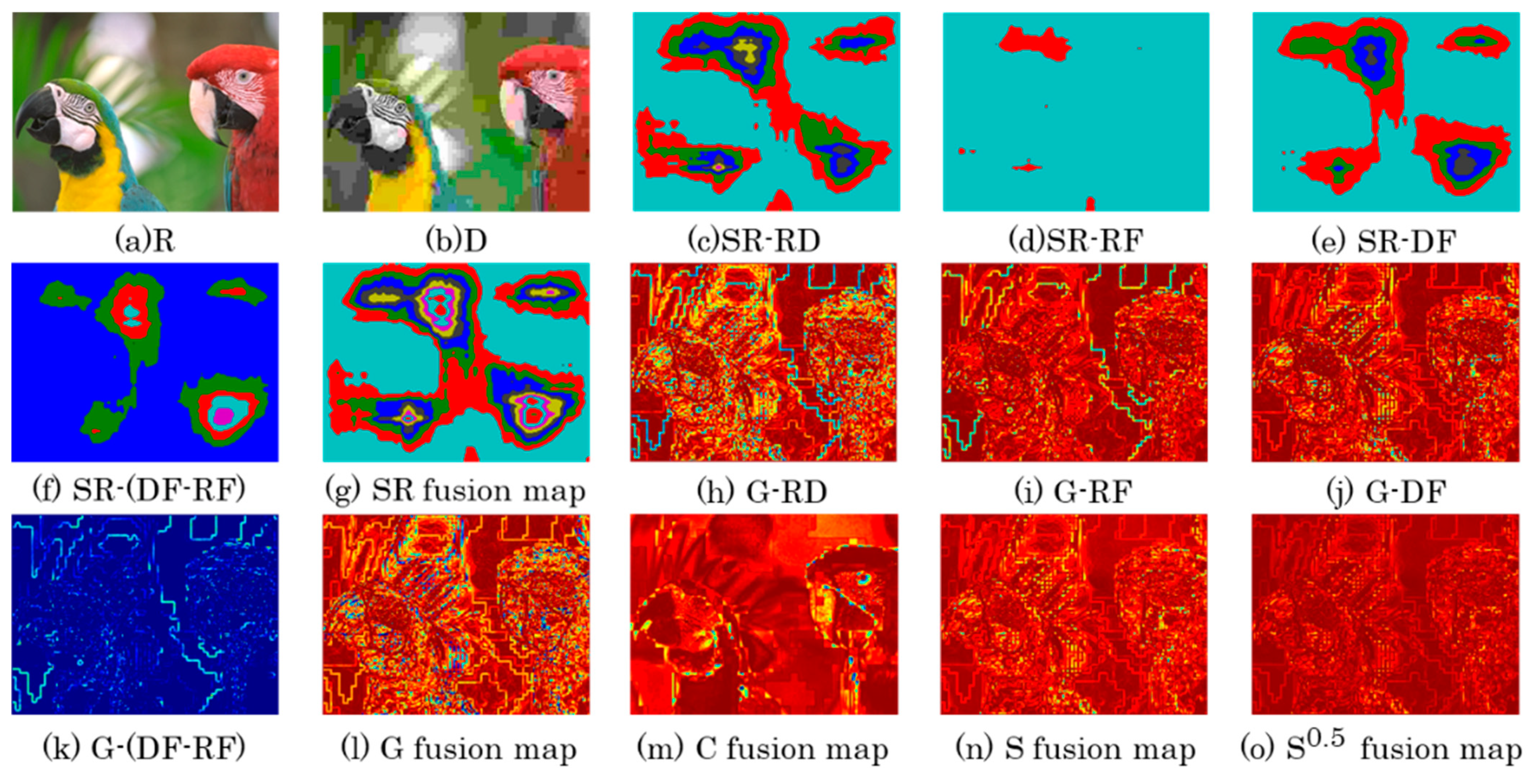
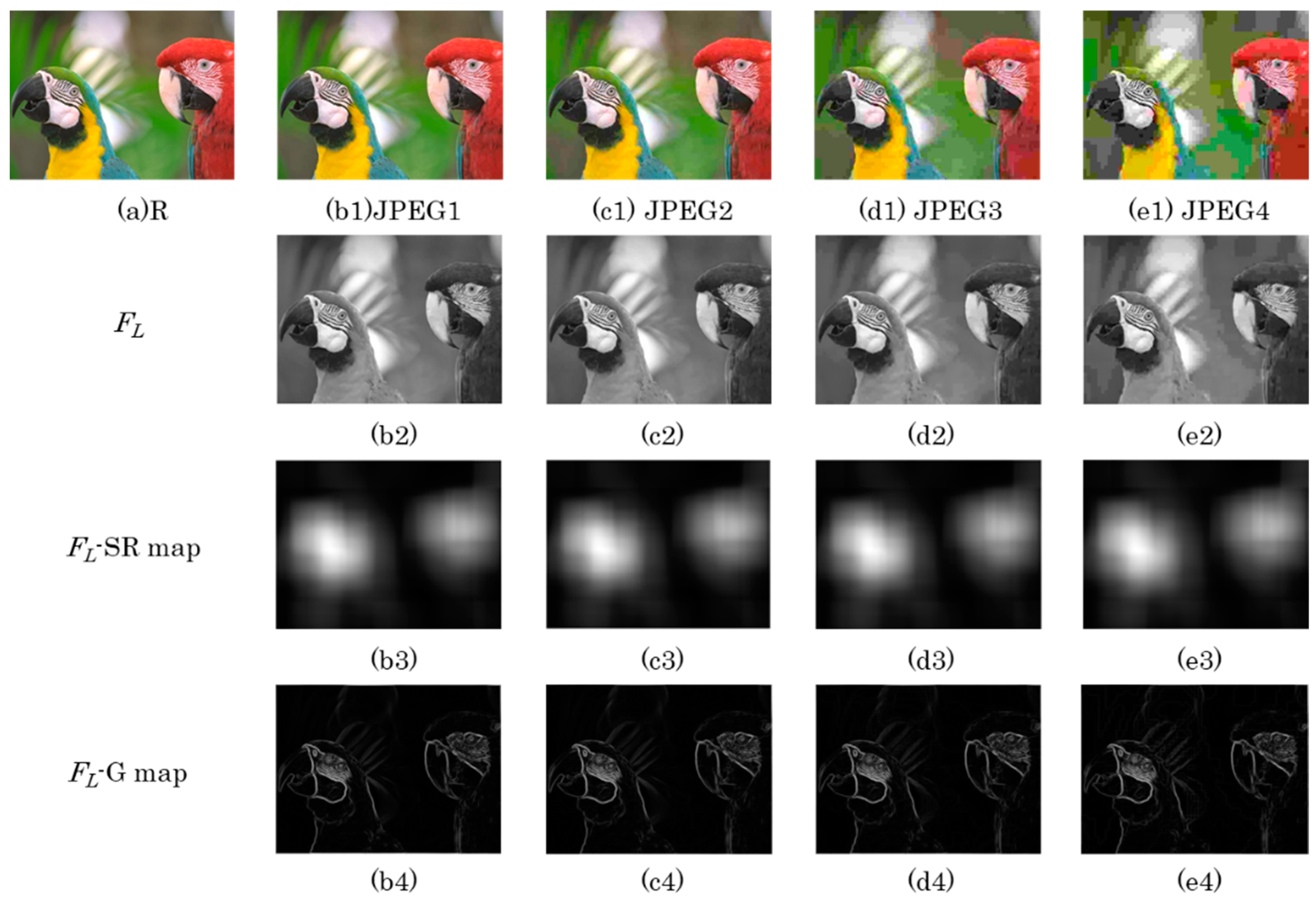
In this article, a reliable FR-IQA method involving similarity calculation is developed without learning. The proposed method connects three feature information processing components, i.e., visual saliency, gradient, and chromatic features, by using an MDSI fusion strategy in LMN color space. This fusion strategy consists of three fusion steps and these three fusion steps include luminance channels fusion, similarity maps fusion, and features fusion. After some experimental comparisons with the other outstanding methods, the proposed method is shown to be less complex and to offer better quality predictions.

2. Proposed IQA Methods

In this section, an FR-IQA method to evaluate color image quality is introduced. The proposed method is designed for general purpose, which means that it performs consistently with commonly encountered distortions. Three fusion steps are included in the proposed method. The first fusion step is to fuse the luminance channels of the two images with a fusion weight coefficient for SR and gradient feature extraction. The second fusion step is to calculate the SR and gradient normal similarity maps between two references, distortion and fusion images, and connect these normal similarity maps as SR and gradient [17] fusion similarity maps. In addition, a chrominance fusion similarity map is extracted from the chrominance channels and utilized to represent the color distortion at pixel level [17]. Finally, these three similarity maps mentioned above are combined with different weights and pooled based on the Minkowski pooling method [25].

2.1. Luminance Channels Fusion

Based on related research [20], SR and gradient features are all extracted by the luminance channel of images. In a color image [20], an SR map and a gradient map cannot work quite so well for color distortion types. Hence, to deal with color distortion, chrominance features should be computed specially in an IQA method. Consequently, an RGB color image will be transformed into an opponent color space by Equation (1) [26], which is more compatible with HVS intuition.

$$\left[\begin{array}{c}L\\ M\\ N\end{array}\right]=\left[\begin{array}{ccc}0.06& 0.63& 0.27\\ 0.30& 0.04& -0.35\\ 0.34& -0.6& 0.17\end{array}\right]\left[\begin{array}{c}R\\ G\\ B\end{array}\right]$$

(1)

In LMN color space, L means the luminance channel and M and N represent the chrominance channels. Because of the shortcomings of conventional similarity maps, similarity maps should not compute two independent images in normal way. Inspired by [17], the first step of features fusion in this research, luminance channels of the reference and the distorted images are fused as an FL map for feature enhancement extraction. The fusion strategy is based on a weight coefficient, and it can be calculated by:

$$F_L=\alpha ·\left(R_L+D_L\right)$$

(2)

where RL and DL are the luminance channels of the reference and the distorted images, respectively. α represents the fusion weight and FL is the fusion map. In Figure 1, some example images are selected from the TID2008 database to illustrate the validity of FL maps. Figure 1a is a reference image R and Figure 1(b1–e1) are four JPEG compression images with distortion levels increasing, while Figure 1(b2–e2) represent the FL maps among the images in the first row. It can be clearly seen that the quality of the FL map is lower when the distortion level is higher. In FL maps, some weaker edges in the background region are smoothed, especially in Figure 1(e2). Figure 1(b3–e3) represent the SR maps of the images in the second row after normalization, and Figure 1(b4–e4) are the gradient maps of the images in the second row. It can be observed that there are no obvious differences among the SR maps, whereas the gradient map presents more structural features losing as the image becomes more distorted. As we all know, the SR map indicates the visual attention of an image, and the gradient map can represent the edge features well. After luminance channels fusion, the stronger edges in the texture region will not change obviously and some information in the flat region can be changed. So, the changes in visual saliency features in the SR map cannot be figured out easily and the flat region in the gradient maps may exhibit apparent differences. In the next subsection, the differences in SR maps will be shown by similarity maps calculation.

2.2. Similarity Maps Fusion

The second fusion step is similarity maps fusion. In this subsection, SR, gradient, and chrominance similarity fusion maps are computed in a symmetric way for the reference and distorted images. To extract visual saliency features, the SR operator is selected to process the input images. The prominent advantage of this index is its higher computing efficiency. Different from other SR-based IQA methods [20,24], the fusion similarity map of SR will be calculated with the following equations:

$$S_{SR1}=\frac{2S{R}_R·S{R}_D+K_{SR1}}{S{R}_R^2+S{R}_D^2+K_{SR1}}$$

(3)

$$S_{SR2}=\frac{2S{R}_R·S{R}_F+K_{SR2}}{S{R}_R^2+S{R}_F^2+K_{SR2}}$$

(4)

$$S_{SR3}=\frac{2S{R}_F·S{R}_D+K_{SR3}}{S{R}_F^2+S{R}_D^2+K_{SR3}}$$

(5)

$$S_{SR}=S_{SR1}+S_{SR3}-S_{SR2}$$

(6)

where parameters K_SR1, K_SR2, and K_SR3 are the constants to control numerical stability. These three parameters are set as K_SR1 = 2K_SR2 = 2K_SR3 in the experimental calculation. SR_R, SR_D, and SR_F are the SR maps of reference, distorted images, and the F_L map. Figure 2c–f are the SR similarity maps between R and D, R and the F_L map (RF), D and the F_L map (DF), and DF–RF, respectively. Figure 2g is the fused similarity map of the SR visual saliency feature. After DF–RF computing, the main difference located in the flat region is enlarged. It can be seen that the fused SR similarity map contains more information than the other non-fused ones, especially in the flat region. Based on this, the fused SR similarity map can be a useful feature operator in designing the proposed method.

To compute the image gradient, several operators can be selected, such as the Prewitt operator [27], the Sobel operator [27], the Roberts operator [28], and the Scharr operator [28]. The vertical gradient of an image X is calculated by G_y = g_y ∗ X (see Equation (7)). Similarly, the horizontal gradient is processed by G_x = g_x ∗ X (see Equation (8)). In these two equations, g_x and g_y are horizontal and vertical gradient operators and ∗ represents the convolution. Therefore, the gradient magnitude of an image is defined as $G\left(x\right)=\sqrt{G_x^2+G_y^2}$.

$$G_x=\frac{1}{3}\left[\begin{array}{ccc}1& 0& -1\\ 1& 0& -1\\ 1& 0& -1\end{array}\right]\ast \mathbf{X}$$

(7)

$$G_y=\frac{1}{3}\left[\begin{array}{ccc}1& 1& 1\\ 0& 0& 0\\ -1& -1& -1\end{array}\right]\ast \mathbf{X}$$

(8)

In this article, the Prewitt operator is used to deal with the gradient feature of the L channel in LMN color space among the reference, distorted images and the F_L map, which are G_R, G_D, and G_F, respectively. Then, the gradient fusion similarity map (S_G) is processed by the following the SSIM-based equations and the simple fusion strategy:

$$S_{G1}=\frac{2G_R·G_D+K_{G1}}{G_R^2+G_D^2+K_{G1}}$$

(9)

$$S_{G2}=\frac{2G_R·G_F+K_{G2}}{G_R^2+G_F^2+K_{G2}}$$

(10)

$$S_{G3}=\frac{2G_F·G_D+K_{G3}}{G_F^2+G_D^2+K_{G3}}$$

(11)

$$S_G=S_{G1}+S_{G3}-S_{G3}$$

(12)

where parameters K_G1, K_G2, and K_G3 are the constants to control numerical stability and K_G2 and K_G3 are defined as the same value. Gradient similarity has been widely used in the related literatures [3,8,9,16,17,20,21,22,23,24]. To achieve a better performance, gradient similarity has been extensively investigated in [29]. Gradient fusion similarity was proposed in [17]. Figure 2h–k are the gradient similarity maps between R and D, R and the F_L map (RF), D and the F_L map (DF), and DF–RF, respectively. Figure 2l is the fused similarity map of the gradient. After DF–RF calculation, the main difference located at the weak edge region is enlarged. It can be observed that the fused gradient similarity map contains more information than other non-fused ones, especially in the weaker edge region. In all, the gradient similarity fusion map is a useful evaluator for the structural distortions.

The last fusion similarity map is of the chromatic components in LMN color space and it can be simply defined as [17]:

$$S_C=\frac{2M_R·M_D+2N_R·N_D+K_C}{M_R^2+M_D^2+N_R^2+N_D^2+K_C}$$

(13)

where the parameter K_C is a constant to control numerical stability. Figure 2m is the chrominance fusion similarity map of the reference and the distorted images.

2.3. Features Fusion

The last fusion step is to combine the above three similarity fusion maps. The SR, gradient, and chrominance similarity fusion maps are calculated by the following summation scheme:

$$S=0.4·S_{SR}+0.4·S_G+0.2·S_C$$

(14)

In Equation (14), the three components of the features fusion map have different weight settings in an S map computing procedure. These values are determined by the visual mechanism, since the HVS is generally more sensitive to achromatic features than to chromatic features [30]. The sum of the weight value should be set as 1 and the weight value of achromatic features can be twice as high as chromatic features. Since the SR and gradient features are all achromatic features, extracted in the luminance channel, the weight values of these two features should be set the same. Thus, the weight values of the three parts are set in Equation (14). Figure 2n is the features fusion map. After the three similarity fusion maps are connected, the features fusion map can represent the difference between R and D well.

2.4. Pooling Strategy

After the three fusion steps mentioned above have been finished, the next step in the proposed method is to choose the pooling strategy. Minkowski pooling has proved to be an efficient method for IQA score calculation [17]. With SR, gradient, and chrominance fused similarity maps connected, a novel method in the IQA task is defined and is named the Features Fusion Similarity index (FFS). It is to be described using the following formula:

$$FFS={\left[\frac{1}{n}{\displaystyle \sum _i^n\left|S_i^{0.5}-\left(\frac{1}{n}{\displaystyle \sum _i^n{S}_i^{0.5}}\right)\right|}\right]}^{0.15}$$

(15)

where n is the total pixel number of the S map and S_i is the pixel value of the S map. The open-source MATLAB code of FFS is publicly available online at https://github.com/AlAlien/FFS (accessed on 20 March 2022). The computational framework of FFS is illustrated in Figure 3. Since FFS consists of different features from other IQA methods, the parameters of the pooling method should be set at different values and the values have been shown in Equation (15). Figure 2o is the square root of the S map and it has more distinguishable information than the S map. To prove the effectiveness of FFS, the IQA scores of FFS have been computed for Figure 1(b1–e1). The MOSs for Figure 1(b1–e1) are 6.3438, 5.2500, 3.8065, and 2.2500, respectively, and the FFS scores for Figure 1(b1–e1) are 0.3470, 0.4065, 0.4876, and 0.5410, respectively. The conclusion is that the FFS scores are consistent with the levels of the distorted images.

In this paper, to apply the proposed method in all databases, K_SR1–K_SR3, K_G1–K_G3, and K_C in the proposed method should be fixed. Additionally, α needs also to be specifically defined for overall databases. Based on previous related research, trial-and-error methods are the most popular way of solving parameter optimization problems. In the following section, these parameters will be defined using a trial-and-error method.

3. Experiments and Performance Analysis

3.1. Databases and Assessment Criteria

In this article, four large-scale, publicly available, single-distortion databases are selected for performance optimization and comparison, i.e., TID2013 [31], TID2008 [32], CSIQ [33], and LIVE [34]. Some representative information for these databases is provided in

Table 1. Benchmark test databases for IQA.

Database	Source Images	Distorted Images	Distortion Types	Observers
TID2013	25	3000	24	971
TID2008	25	1700	17	838
CSIQ	30	866	6	35
LIVE	29	779	5	161

. These databases are designed with some ordinarily encountered distortions in real-world applications of IQA. They are annotated with subjective scores, i.e., MOS or DMOS, as suitable benchmarks between the proposed method and others.

In order to test the IQA performance, comparisons are made between the computed scores and the ratings by humans. Four widely used criteria for the performance comparisons of IQA methods are employed: Spearman rank-order correlation coefficient (SROCC), Pearson linear correlation coefficient (PLCC), Kendall rank-order correlation coefficient (KROCC), and root mean squared error (RMSE) [2,35]. Both SROCC and KROCC are calculated by rank of the score and PLCC takes the relative distance between scores into consideration. PLCC is used to indicate the correlation between subjective evaluation and objective evaluation by logistic regression, and SROCC and KROCC are utilized to measure the consistency between objective evaluation and subjective evaluation values [24]. These three criteria reaching unity 1 means that the prediction performance of an objective method is considered high. For the RMSE, a smaller value represents better performance.

Before computing the PLCC and RMSE, a logistic regression should be utilized to process subjective judgments by means of the following equation:

$$p\left(x\right)={\beta }_1\left[\frac{1}{2}-\frac{1}{1+\exp \left({\beta }_2\left(x-{\beta }_3\right)\right)}\right]+{\beta }_{4}x+{\beta }_5$$

(16)

where β₁, …, β₅ are the parameters to be fitted, x represents the scores computed by the IQA method, and p(x) is the rating after logistic regression [34].

3.2. Parameter Setting for FFS

In this work, there are five main parameters that need to be determined, including α, K_SR1, K_C, K_G1, and K_G2. In the optimizing procedure, when a parameter is tested, the others are fixed as invariable. PLCC is selected as the main criterion to define the parameters because these four criteria perform similarly in parameter optimization experiments.

Parameter α serves as the fusion weight between the luminance channels of reference and distorted images. As shown in Figure 4, PLCC changes with α on the four single-distortion databases presented. The optimal intervals for α on TID2013, TID2008, CSIQ, and LIVE are in [0.5, 0.53], [0.51, 0.55], [0.47, 0.52], [0.5, 0.53]. It can be found that the best fusion weight values are different for each database. In these databases, the optimal α values have similar intervals, which is consistent with visual perception under certain fusion weights in IQA. In this research, α is fixed as 0.52.

Parameters K_SR1 and K_C are the numerical stability controllers for S_SR and S_C. As expressed in Figure 5a, the PLCC and SROCC curves against K_SR1 for the TID2013 database are shown. It can be observed that, for TID2013, the performances are all stable and high when K_SR1 stays in the interval [0.25, 0.75]. In this work, K_SR1 can be set as 0.25. Figure 5b shows the SROCC and PLCC curves against K_C for the TID2013 database. It can be found that, for TID2013, when K_C keeps in [260, 280], the performances can be stable and high. In this research, K_C can be fixed as 270.

K_G1 and K_G2 are the last two parameters, set as the numerical stability controllers for S_G. Their influences on the perfomance of FFS will be studied. Figure 6 illustrates the results by a contour map. It can be found that the optimal K_G1 and K_G2 for TID2013 are in the intervals [140, 180] × [70, 110]. In this article, K_G1 and K_G2 are set as 160 and 90, respectively.

3.3. Overall Performance Comparison

Overall performance comparisons need to be conducted to test the ability of an IQA method with different databases. In this subsection, the performance of the proposed method was compared with eight typical methods, including SSIM [12], FSIMc [16] (the improved FSIM method with color space transforming), and VSI [21], IFS [13], LLM [15], MDSI [17], GDRW [22], EFS [23], and the latest SSVD [18], VCGS [9], SPSIM (YCbCr_MDSI) [3], and GSC [24] published in 2019, 2020, 2021, and 2022, respectively. To show the better performance, the highest three values for all the criteria are highlighted in boldface in

Table 2. Comparison of SROCC values for selected IQA methods.

	TID2013	TID2008	CSIQ	LIVE	W. A.	D. A.
SSIM	0.7417	0.7749	0.8756	0.9601	0.8008	0.8381
FSIMc	0.8510	0.8840	0.9310	0.9807	0.8896	0.9117
VSI	0.8965	0.8979	0.9423	0.9708	0.9141	0.9269
IFS	0.8697	0.8903	0.9581	0.9599	0.9003	0.9195
LLM	0.9037	0.9077	0.9050	0.9608	0.9135	0.9193
MDSI	0.8899	0.9208	0.9569	0.9667	0.9183	0.9336
GDRW	0.8803	0.8971	0.9590	0.9752	0.9093	0.9279
EFS	0.8948	0.8925	0.9371	0.9550	0.9088	0.9199
SSVD	0.8112	0.8846	0.8975	0.9740	0.8661	0.8918
VCGS	0.8926	0.8975	0.9443	0.9768	0.9133	0.9278
SPSIM(YCbCr_MDSI)	0.9067	0.9150	0.9434	0.9625	0.9221	0.9319
GSC	0.8657	0.8906	0.9598	0.9589	0.8986	0.9188
Proposed	0.8926	0.9166	0.9550	0.9768	0.9197	0.9353

,

Table 3. Comparison of PLCC values for selected IQA methods.

	TID2013	TID2008	CSIQ	LIVE	W. A.	D. A.
SSIM	0.7895	0.7732	0.8613	0.9508	0.8190	0.8437
FSIMC	0.8769	0.8762	0.9192	0.9729	0.8967	0.9113
VSI	0.8999	0.8762	0.9279	0.9659	0.9073	0.9175
IFS	0.8791	0.8810	0.9576	0.9586	0.9019	0.9191
LLM	0.9068	0.8971	0.9000	0.9578	0.9110	0.9154
MDSI	0.9080	0.9160	0.9530	0.9659	0.9247	0.9358
GDRW	0.8913	0.8821	0.9541	0.9752	0.9098	0.9257
EFS	0.9067	0.8810	0.9287	0.9506	0.9095	0.9168
SSVD	0.8198	0.8940	0.8878	0.9687	0.8704	0.8926
VCGS	0.9000	0.8776	0.9301	0.9676	0.9083	0.9188
SPSIM (YCbCr_MDSI)	0.9173	0.9051	0.9334	0.9583	0.9224	0.9285
GSC	0.8766	0.8801	0.9601	0.9577	0.9007	0.9186
Proposed	0.9116	0.9168	0.9530	0.9774	0.9283	0.9397

,

Table 4. Comparison of KROCC values for selected IQA methods.

	TID2013	TID2008	CSIQ	LIVE	W. A.	D. A.
SSIM	0.5588	0.5768	0.6907	0.8314	0.6218	0.6644
FSIMC	0.6665	0.6991	0.7690	0.8881	0.7217	0.7557
VSI	0.7183	0.7123	0.7857	0.8517	0.7457	0.7670
IFS	0.6785	0.7009	0.8158	0.8254	0.7245	0.7552
LLM	0.7209	0.7368	0.7238	0.8230	0.7407	0.7511
MDSI	0.7123	0.7515	0.8130	0.8395	0.7549	0.7791
GDRW	0.6978	0.7125	0.8169	0.8660	0.7426	0.7733
EFS	0.7200	0.7091	0.7789	0.8109	0.7386	0.7547
SSVD	0.6467	0.7105	0.7255	0.8601	0.7057	0.7357
VCGS	0.7166	0.7171	0.7906	0.8752	0.7503	0.7749
SPSIM (YCbCr_MDSI)	0.7306	0.7393	0.7877	0.8307	0.7554	0.7721
GSC	0.6764	0.7017	0.8190	0.8212	0.7235	0.7546
Proposed	0.7159	0.7443	0.8111	0.8700	0.7590	0.7853

and

Table 5. Comparison of RMSE values for selected IQA methods.

	TID2013	TID2008	CSIQ	LIVE	W. A.	D. A.
SSIM	0.7608	0.8511	0.1334	9.6902	2.0404	2.8589
FSIMC	0.5959	0.6468	0.1034	7.2367	1.5399	2.1457
VSI	0.5404	0.6466	0.0979	8.1036	1.6437	2.3471
IFS	0.5909	0.6349	0.0757	7.7764	1.6118	2.2695
LLM	0.5277	0.5982	0.1232	7.7678	1.5783	2.2542
MDSI	0.5181	0.5383	0.0796	7.0790	1.4493	2.0538
GDRW	0.5621	0.6322	0.0786	6.9288	1.4712	2.0504
EFS	0.5230	0.6349	0.0973	8.4794	1.6890	2.4337
SSVD	0.7099	0.6013	0.1208	7.7709	1.6627	2.3007
VCGS	0.5404	0.6433	0.0964	7.9035	1.6127	2.2959
SPSIM (YCbCr_MDSI)	0.4935	0.5705	0.0942	7.8048	1.5572	2.2408
GSC	0.5879	0.6332	0.0721	4.7564	1.1566	1.5124
Proposed	0.5096	0.5360	0.0796	6.6203	1.3760	1.9364

. In addition, the weighted average (W. A.) and direct average (D. A.) values of the SROCC, PLCC, and KROCC results of these databases are also included to assess the overall performance, according to Wang and Li [36]. The weight of each database is computed by the number of the distortion images contained in the database.

As shown in Table 2, Table 3, Table 4 and Table 5, it can be concluded that the proposed method has a consistent performance for all the selected databases. Specifically, the proposed method always keeps in the top-three ranks for the TID2008 and LIVE databases. For the TID2013 and CSIQ databases, the gap between the proposed method’s performance and the top three results is very small. Meanwhile, there is no method that performs the best for all databases, based on the distribution of boldfaced figures in Table 2, Table 3, Table 4 and Table 5. From the results for each element of the performance comparisons of IQA methods, it can be found that the effective methods are the proposed method, SPSIM(YCbCr_MDSI), and MDSI on SROCC; for PLCC, the proposed method, MDSI, and SPSIM(YCbCr_MDSI) provide precise results; the proposed method, MDSI, and SPSIM(YCbCr_MDSI) perform IQA consistently with human opinion scores on KROCC; as for RMSE, the proposed method, GSC, GDRW, and MDSI have better performances than the others. Furthermore, the proposed method also has the best performance for the weighted and direct average values. From Table 2, the accuracy SROCC of the proposed method can achieve 0.8926 at least and 0.9768 at most for all databases. From Table 3, the accuracy PLCC value of the proposed method can achieve 0.9116 at least and 0.9774 at most for four databases. Moreover, the proposed method yields the best rank of the weighted average values of PLCC and KROCC, and the direct average values of SROCC, PLCC, and KROCC. Furthermore, the proposed method yields the best rank number (18 times) among chosen IQA methods, followed by MDSI (13 times), and SPSIM(YCbCr_MDSI) (13 times).

From Table 2, Table 3, Table 4 and Table 5, it can be seen that the proposed method yields better performance than the learning-based methods, i.e., IFS and LLM. Meanwhile, the proposed method performs better than the methods without color space transforming, i.e., SSIM and SSVD. In the selected methods with color space transforming, some of them contain normal gradient maps, i.e., FSIMc, VSI, GDRW, EFS, and VCGS. Compared with these methods, the proposed method with a fusion gradient map has remarkable advantages for all databases. As for the methods consisting of fusion gradient maps, i.e., MDSI, SPSIM(YCbCr_MDSI), and GSC, it can be found that IQA performance is improved by fusing SR, gradient, and chrominance features in three fusion steps.

3.4. Performance Comparison among Different Distortion Types and Statistical Significance Comparisons

The performance comparison among different distortion types should be carried out to check the IQA method’s ability to predict image quality. In

Table 6. SROCC values of IQA methods for each type of distortion.

Databases	Distortion Type	SSIM	FSIMC	VSI	IFS	LLM	MDSI	GDRW	EFS	SSVD	VCGS	GSC	Proposed
TID2013	AGN	0.8671	0.9101	0.9460	0.9382	0.9462	0.9477	0.9470	0.9427	0.9221	0.9368	0.9120	0.9503
	ANC	0.7726	0.8537	0.8705	0.8537	0.8975	0.8794	0.8675	0.8680	0.8289	0.8559	0.9352	0.8820
	SCN	0.8515	0.8900	0.9367	0.9340	0.9349	0.9459	0.9386	0.9369	0.9369	0.9315	0.9435	0.9491
	MN	0.7767	0.8094	0.7697	0.7960	0.7545	0.8004	0.7116	0.7943	0.7325	0.8070	0.8898	0.7962
	HFN	0.8634	0.9094	0.9200	0.9140	0.9524	0.9147	0.9178	0.9209	0.8995	0.9162	0.9258	0.9192
	IN	0.7503	0.8251	0.8741	0.8389	0.8326	0.8600	0.8038	0.8861	0.7671	0.8682	0.9046	0.8653
	QN	0.8657	0.8807	0.8748	0.8335	0.9055	0.9015	0.8955	0.8682	0.8572	0.8831	0.7585	0.8841
	GB	0.9668	0.9551	0.9612	0.9658	0.9451	0.9523	0.9206	0.9631	0.9499	0.9549	0.9704	0.9565
	DEN	0.9254	0.9330	0.9484	0.9183	0.9478	0.9498	0.9539	0.9473	0.9486	0.9454	0.9497	0.9508
	JPEG	0.9200	0.9339	0.9541	0.9290	0.9544	0.9504	0.9513	0.9520	0.9318	0.9597	0.9627	0.9487
	JP2K	0.9468	0.9589	0.9706	0.9611	0.9702	0.9635	0.9657	0.9707	0.9688	0.9686	0.9542	0.9641
	JPTE	0.8493	0.8610	0.9216	0.8925	0.8459	0.8897	0.8847	0.9241	0.8441	0.8955	0.9003	0.8990
	J2TE	0.8828	0.8919	0.9228	0.9010	0.9176	0.9098	0.9174	0.9233	0.9332	0.9204	0.8790	0.9167
	NEPN	0.7821	0.7937	0.8060	0.7839	0.7967	0.8217	0.8137	0.8201	0.8085	0.7887	0.8976	0.8123
	Block	0.5720	0.5532	0.1713	0.1004	0.6273	0.6931	0.2627	0.5581	0.4768	0.4326	0.7455	0.6455
	MS	0.7752	0.7487	0.7700	0.6575	0.7586	0.7424	0.7597	0.7821	0.7504	0.7646	0.7683	0.7752
	CTC	0.3775	0.4679	0.4754	0.4469	0.4634	0.4378	0.3795	0.4748	0.4494	0.4687	0.7819	0.4913
	CCS	0.4141	0.8359	0.8100	0.8257	0.3117	0.8001	0.7980	0.8261	0.3562	0.7816	0.6366	0.8096
	MGN	0.7803	0.8569	0.9117	0.8790	0.9097	0.8897	0.8904	0.9051	0.8600	0.8948	0.9266	0.8987
	CN	0.8566	0.9135	0.9243	0.9037	0.9455	0.9190	0.9302	0.9192	0.9263	0.9268	0.9114	0.9241
	LCNI	0.9057	0.9485	0.9564	0.9433	0.9588	0.9559	0.9631	0.9550	0.9649	0.9556	0.9172	0.9594
	ICQD	0.8542	0.8815	0.8839	0.9007	0.9155	0.9134	0.9044	0.9007	0.8948	0.9050	0.9002	0.9112
	CHA	0.8775	0.8925	0.8906	0.8862	0.8682	0.8824	0.8609	0.8954	0.8816	0.8861	0.8837	0.8861
	SSR	0.9461	0.9576	0.9628	0.9556	0.9676	0.9638	0.9667	0.9630	0.9700	0.9635	0.9345	0.9635
CSIQ	AWGN	0.8974	0.9359	0.9636	0.9593	0.9403	0.9676	0.9686	0.9671	0.9474	0.9671	0.9588	0.9661
	JPEG	0.9543	0.9664	0.9618	0.9660	0.9602	0.9572	0.9669	0.9672	0.9593	0.9643	0.9660	0.9581
	JP2K	0.9605	0.9704	0.9694	0.9712	0.9730	0.9732	0.9751	0.9772	0.9692	0.9747	0.9713	0.9772
	AGPN	0.8924	0.9370	0.9638	0.9526	0.9241	0.9665	0.9623	0.9604	0.9392	0.9624	0.9389	0.9640
	GB	0.9608	0.9729	0.9679	0.9621	0.9650	0.9733	0.9730	0.9774	0.9713	0.9734	0.9789	0.9778
	CTC	0.7925	0.9438	0.9504	0.9485	0.9418	0.9446	0.9282	0.9557	0.8690	0.9553	0.9145	0.9488
LIVE	JP2K	0.9614	0.9724	0.9604	0.9694	0.9668	0.9703	0.9697	0.9678	0.9681	0.9841	0.9726	0.9786
	JPEG	0.9764	0.9840	0.9761	0.9778	0.9735	0.9762	0.9805	0.9767	0.9805	0.9849	0.9867	0.9758
	AWGN	0.9694	0.9716	0.9835	0.9883	0.9765	0.9871	0.9811	0.9841	0.9816	0.9896	0.9850	0.9905
	GB	0.9517	0.9708	0.9527	0.9665	0.9529	0.9673	0.9575	0.9663	0.9387	0.9763	0.9765	0.9787
	FF	0.9556	0.9519	0.9430	0.9404	0.9452	0.9487	0.9450	0.9490	0.9392	0.9683	0.9489	0.9669

, the comparison results for different distortion types are summarized. The tests on TID2008 are not displayed, since all distortion types of TID2008 are contained in the TID2013 database. The performance measurement was chosen as SROCC because it had a similar effect to the other criteria, i.e., PLCC, RMSE, and KROCC. Therefore, these three databases contained 35 distortion types of images to be compared. Due to the lack of an open-source code, the results of SPSIM(YCbCr_MDSI) are not included in Table 6, and the results of GSC are based on the values from the published paper. The top three SROCC values of all distortion types are highlighted in bold to show the ability of IQA. From Table 6, the proposed method (17 times) wins the best SROCC-performance rank, followed by GSC (15 times), EFS (14 times), VCGS (11 times), GDRW (10 times), and MDSI (9 times). Furthermore, their performances are much better than other IQA methods. Meanwhile, there is no method that performs the best for all distortion types. The proposed method cannot deal with some distortion types, e.g., MN, NEPN, Block, or CTC in TID2013. Compared with MDSI, the proposed method performs much better for the performance comparison among different distortion types. In a comparison of the proposed method and GSC, GSC has a much better performance with respect to MN, NEPN, Block, and CTC in TID2013, while the proposed method performs much better for AGN, QN, CCS, and LCNI in TID2013. To sum up, the conclusion is that the proposed IQA method performs better than others depending on the distortion type.

There are some scatter plots shown in Figure 7 for the TID2013 database based on the open-source code mentioned in the articles. Due to the lack of an open-source code, the scatter plots of SPSIM(YCbCr_MDSI) and GSC are not included in Figure 7. To compare the visual performance between the proposed method and the comparison methods, the scatter plot for the proposed method is shown in Figure 8. It can be concluded that the proposed method performs consistently with the subjective ratings, compared with most IQA methods, including MDSI.

Moreover, statistical significance comparisons were performed and the results are displayed in

Table 7. Statistical significance comparison of different IQA methods.

Database	SSIM	FSIMc	VSI	IFS	LLM	MDSI	GDRW	EFS	SSVD	VCGS
CSIQ	1	1	1	0	1	0	0	1	1	1
LIVE	1	1	1	1	1	0	0	1	1	1
TID2008	1	1	1	1	0	0	1	1	1	1
TID2013	1	1	1	1	0	0	1	1	1	1

. These values were computed by means of a series of hypothetical experiments to evaluate the residuals of all methods after logistic regression [2,35]. In particular, the left-tailed F-test was used to pairwise test between the proposed method and other methods. In this article, the left-tailed F-test was set at a 0.05 significance level. After the calculation, the result H = 1 (green) means that the first method (the proposed method) yields a better IQA performance than the second method (the method in the first row of Table 7) with a confidence larger than 95%. A value of H = 0 (orange) shows that these two competing methods have similar IQA performances. As shown in Table 7, the number of total statistical tests between two methods is 40 and the number of comparisons in which the proposed method surpasses the others statistically is 31. Therefore, the proposed method yields significant improvement in 77.5% of the cases. Consequently, the proposed method has been shown to have a very promising statistical performance when compared with most of the other methods.

In this subsection, with the fusion gradient map, the proposed method shows an obvious improvement for the different distortion types and statistical significance tests, compared with the methods containing the normal gradient map, including FSIMc, GSM, VSI, GDRW, EFS, and VCGS. Compared with MDSI, it can be concluded that IQA performance is improved by the proposed method among different distortion type comparisons, and the proposed method has a similar performance among the statistical significance tests. Compared with GSC, the performance with different distortion types has been obviously improved by the fusion strategy utilized in the proposed method. Therefore, it can be concluded that the proposed method has better predictive accuracy than the other IQA methods with respect to the widely used databases.

3.5. Computational Cost

Computational cost is another criterion for assessing all IQA methods, which represents computational efficiency. All the experiments in this research were conducted on a PC with a 2.5 GHz Intel Core i5 CPU and 8 G RAM running the MATLAB R2013b software platform and included a running time comparison. The average running times of each method for the TID2013 database, with a resolution of 512 × 384, are listed in

Table 8. Time cost of each IQA method.

Methods	SSIM	FSIMc	VSI	IFS	MDSI	GDRW	EFS	SSVD	VCGS	FFS
Time(s)	0.0601	0.3110	0.2727	0.0771	0.0255	4.6298	1.6161	0.1886	0.6240	0.0657

(the running time of FFS is in bold). It can be observed that the FFS is less computationally complex than most IQA methods. The running time of MDSI and SSIM are lower than the proposed method but the proposed method has a higher predictive accuracy. In the experiments, it can be found that the time cost of the proposed method is about 0.0657 s. Hence, FFS can be used for a real-time automated system application with a higher computational efficiency. To deal with the IQA problem in real settings, the importance of computational cost and prediction accuracy should be at the same level.

4. Conclusions

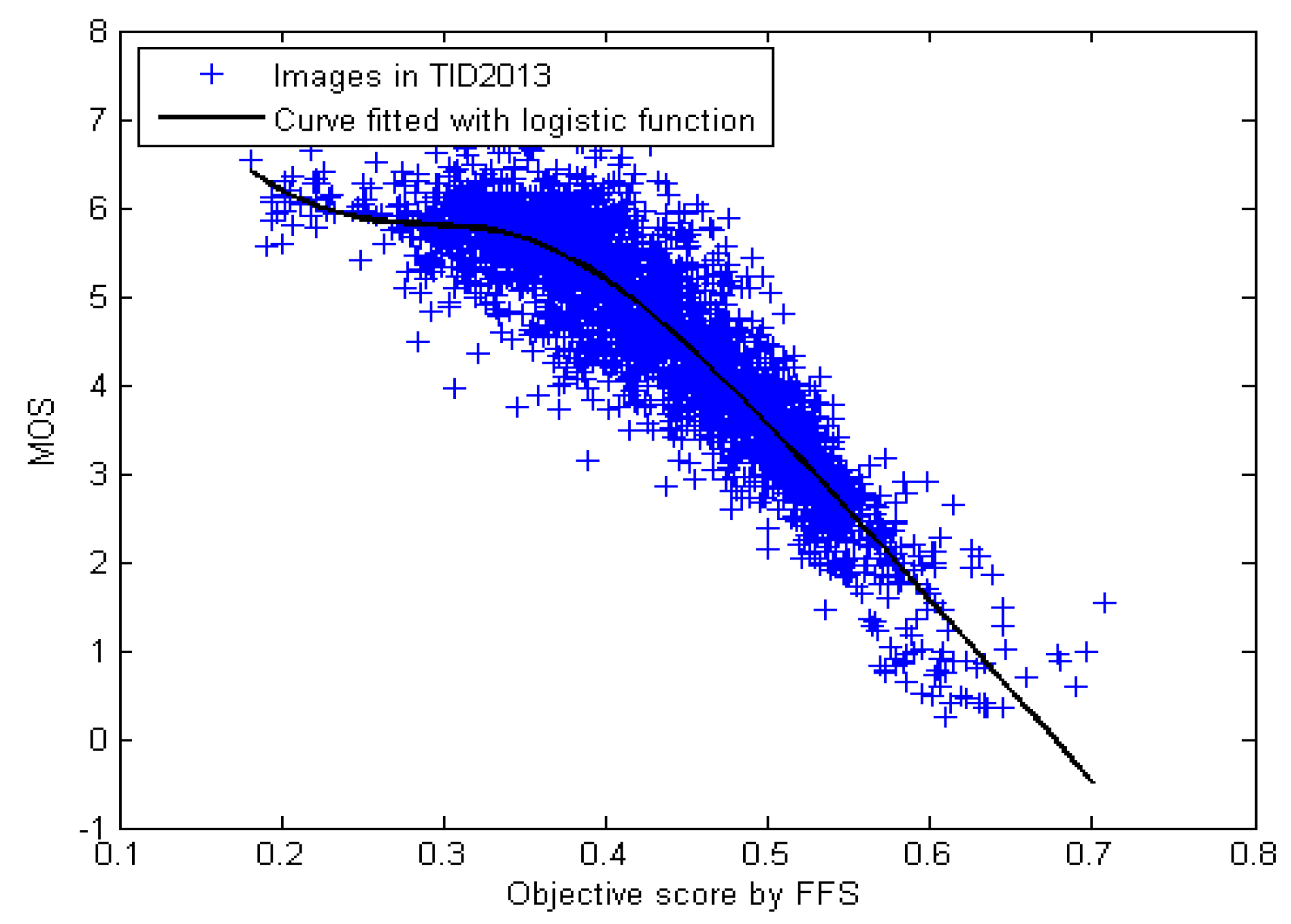
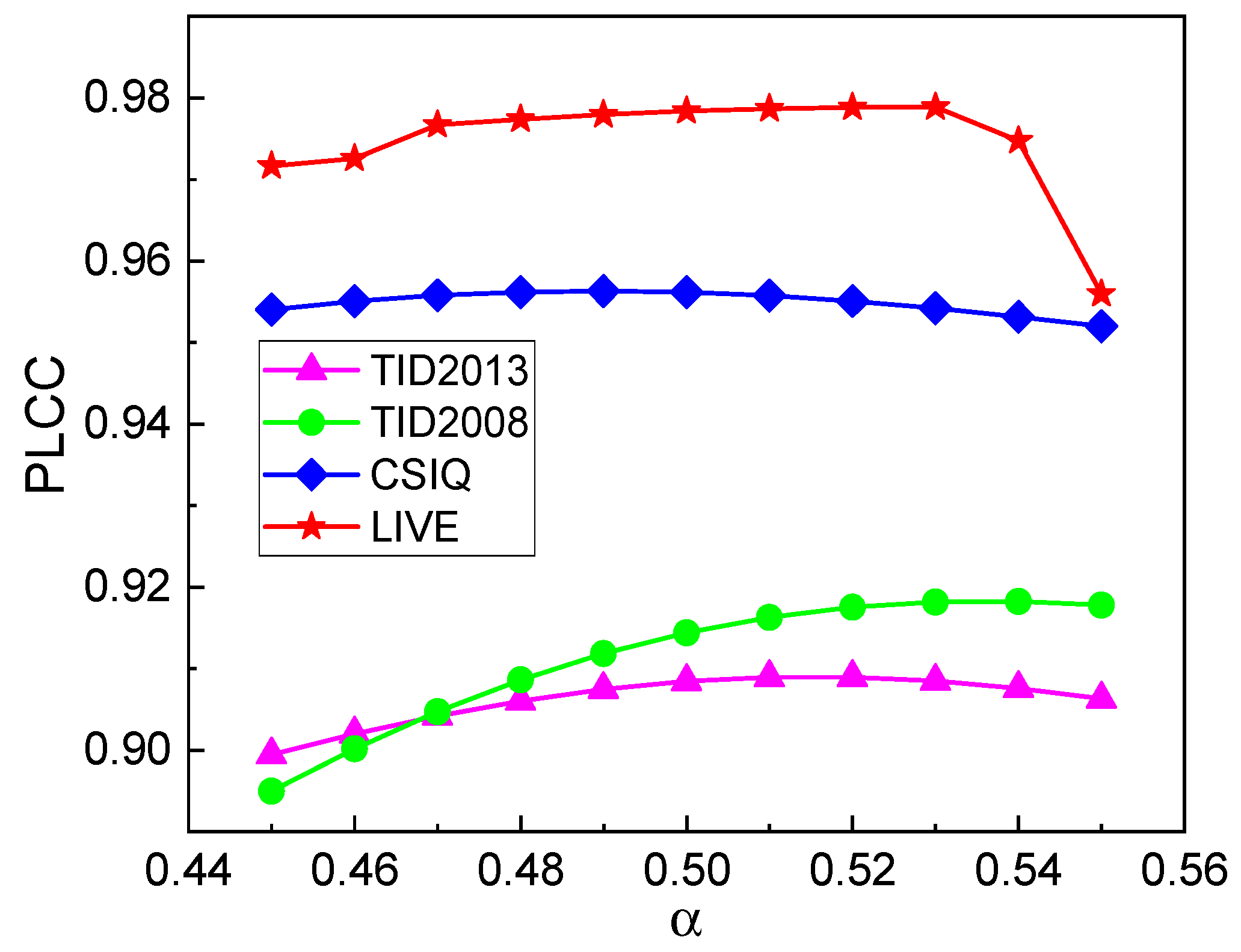
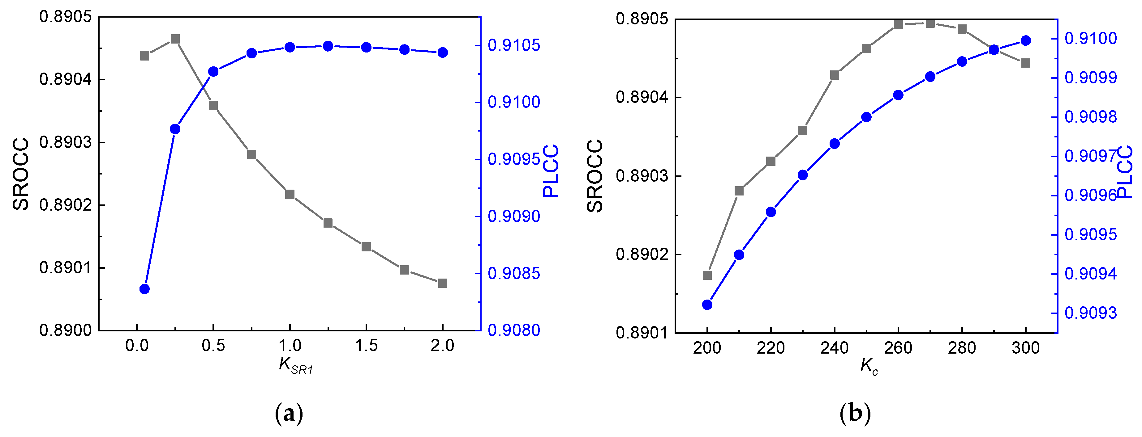
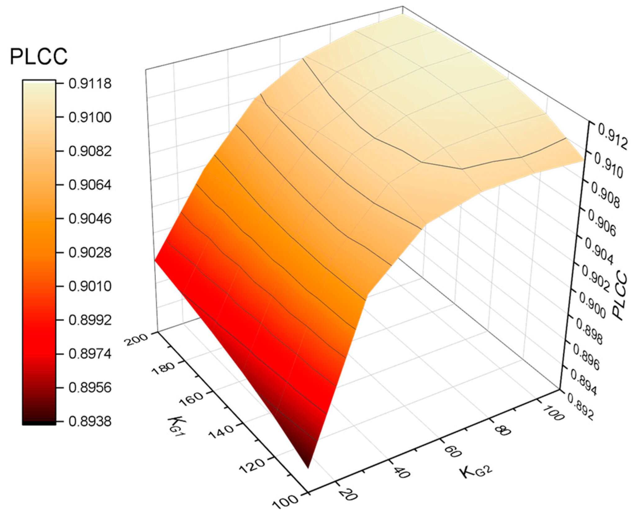
In this research, a novel FR-IQA method with good performance was proposed, namely, the features fusion similarity (FFS) method. This method consists of three fusion steps, i.e., luminance fusion, similarity maps fusion, and features fusion. Firstly, the luminance channels of two images are fused with a fusion weight for SR and gradient features enhancement extraction. Secondly, the reference image, the distorted image, and fusion map were calculated by means of a SR similarity fusion map, a gradient similarity fusion map and a chrominance similarity fusion map in a symmetric way, respectively. Lastly, these three feature similarity maps were fused with different weights based on the HVS mechanism and then a deviation pooling strategy was selected to process the features fusion map to obtain an image quality score. After the IQA method design, the main parameters were defined by optimization tests. Twelve state-of-the-art or newly published IQA methods were selected as methods to put in competition with the proposed method with respect to four popular databases. The experimental results showed that the accuracy PLCC value of FFS can achieve at least 0.9116 and at most 0.9774 for the four databases. The time cost of the proposed method is about 0.0657 s. These comparative results illustrated that FFS yields statistically better predictive accuracy than the other methods with a higher computational efficiency. In the future, all IQA methods need to be improved to yield a better performance for the IQA problem in real settings, including the proposed method.

References

1. Zhan, Y.B.; Zhang, R.; Wu, Q. A Structural Variation Classification Model for Image Quality Assessment. IEEE Trans. Multimed. 2017, 19, 1837–1847. [Google Scholar] [CrossRef]
2. Athar, S.; Wang, Z. A Comprehensive Performance Evaluation of Image Quality Assessment Algorithms. IEEE Access 2019, 7, 140030–140070. [Google Scholar] [CrossRef]
3. Frackiewicz, M.; Szolc, G.; Palus, H. An Improved SPSIM Index for Image Quality Assessment. Symmetry 2021, 13, 518. [Google Scholar] [CrossRef]
4. Saha, A.; Wu, Q.M.J. Full-reference image quality assessment by combining global and local distortion measures. Signal Process. 2016, 128, 186–197. [Google Scholar] [CrossRef] [Green Version]
5. Saha, A.; Wu, Q.M.J. Perceptual image quality assessment using phase deviation sensitive energy features. Signal Process. 2013, 93, 3182–3191. [Google Scholar] [CrossRef]
6. Zhou, B.Z.; Shao, F.; Meng, X.C.; Fu, R.D.; Ho, Y.S. No-Reference Quality Assessment for Pansharpened Images via Opinion-Unaware Learning. IEEE Access 2019, 7, 40388–40401. [Google Scholar] [CrossRef]
7. Lin, W.S.; Kuo, C.C.J. Perceptual visual quality metrics: A survey. J. Vis. Commun. Image Represent. 2011, 22, 297–312. [Google Scholar] [CrossRef]
8. Shi, C.-Y.; Lin, Y.-D. Objective image quality assessment based on image color appearance and gradient features. Acta Phys. Sin. 2020, 69, 228701. [Google Scholar] [CrossRef]
9. Shi, C.Y.; Lin, Y.D. Full Reference Image Quality Assessment Based on Visual Salience With Color Appearance and Gradient Similarity. IEEE Access 2020, 8, 97310–97320. [Google Scholar] [CrossRef]
10. Reisenhofer, R.; Bosse, S.; Kutyniok, G.; Wiegand, T. A Haar wavelet-based perceptual similarity index for image quality assessment. Signal Process-Image 2018, 61, 33–43. [Google Scholar] [CrossRef] [Green Version]
11. Wang, R.F.; Yang, H.; Pan, Z.K.; Huang, B.X.; Hou, G.J. Screen Content Image Quality Assessment With Edge Features in Gradient Domain. IEEE Access 2019, 7, 5285–5295. [Google Scholar] [CrossRef]
12. Wang, Z.; Bovik, A.C.; Sheikh, H.R.; Simoncelli, E.P. Image quality assessment: From error visibility to structural similarity. IEEE Trans. Image Process. 2004, 13, 600–612. [Google Scholar] [CrossRef] [PubMed] [Green Version]
13. Chang, H.W.; Zhang, Q.W.; Wu, Q.G.; Gan, Y. Perceptual image quality assessment by independent feature detector. Neurocomputing 2015, 151, 1142–1152. [Google Scholar] [CrossRef]
14. Hyvarinen, A. Fast and robust fixed-point algorithms for independent component analysis. IEEE Trans. Neural Netw. 1999, 10, 626–634. [Google Scholar] [CrossRef] [Green Version]
15. Wang, H.; Fu, J.; Lin, W.; Hu, S.; Kuo, C.-C.J.; Zuo, L. Image quality assessment based on local linear information and distortion-specific compensation. IEEE Trans. Image Process. 2016, 26, 915–926. [Google Scholar] [CrossRef]
16. Zhang, L.; Zhang, L.; Mou, X.Q.; Zhang, D. FSIM: A Feature Similarity Index for Image Quality Assessment. IEEE Trans. Image Process. 2011, 20, 2378–2386. [Google Scholar] [CrossRef] [Green Version]
17. Nafchi, H.Z.; Shahkolaei, A.; Hedjam, R.; Cheriet, M. Mean Deviation Similarity Index: Efficient and Reliable Full-Reference Image Quality Evaluator. IEEE Access 2016, 4, 5579–5590. [Google Scholar] [CrossRef]
18. Mansouri, A.; Mahmoudi-Aznaveh, A. SSVD: Structural SVD-based image quality assessment. Signal Process-Image 2019, 74, 54–63. [Google Scholar] [CrossRef]
19. Hou, X.; Zhang, L. Saliency Detection: A Spectral Residual Approach. In Proceedings of the 2007 IEEE Computer Society Conference on Computer Vision and Pattern Recognition (CVPR 2007), Minneapolis, MN, USA, 17–22 June 2007; pp. 2280–2287. [Google Scholar] [CrossRef]
20. Zhang, L.; Li, H.Y. SR-SIM: A fast and high performance IQA index based on spectral residual. In Proceedings of the 2012 IEEE International Conference on Image Processing (ICIP), Orlando, FL, USA, 30 September–3 October 2012; pp. 1473–1476. [Google Scholar] [CrossRef]
21. Zhang, L.; Shen, Y.; Li, H.Y. VSI: A Visual Saliency-Induced Index for Perceptual Image Quality Assessment. IEEE Trans. Image Process. 2014, 23, 4270–4281. [Google Scholar] [CrossRef] [Green Version]
22. Shi, Z.F.; Chen, K.X.; Pang, K.; Zhang, J.P.; Cao, Q.J. A perceptual image quality index based on global and double-random window similarity. Digit. Signal Process. 2017, 60, 277–286. [Google Scholar] [CrossRef]
23. Shi, Z.; Zhang, J.; Cao, Q.; Pang, K.; Luo, T. Full-reference image quality assessment based on image segmentation with edge feature. Signal Process. 2018, 145, 99–105. [Google Scholar] [CrossRef]
24. Chang, H.-W.; Bi, X.-D.; Du, C.-Y.; Mao, C.-W.; Wang, M.-H. Image Quality Evaluation Based on Gradient, Visual Saliency, and Color Information. Int. J. Digit. Multimed. Broadcast. 2022, 2022, 7540810. [Google Scholar] [CrossRef]
25. Wang, Z.; Shang, X.L. Spatial pooling strategies for perceptual image quality assessment. In Proceedings of the 2006 IEEE International Conference on Image Processing, ICIP 2006, Atlanta, GA, USA, 8–11 October 2006; pp. 2945–2948. [Google Scholar] [CrossRef] [Green Version]
26. Geusebroek, J.M.; van den Boomgaard, R.; Smeulders, A.W.M.; Geerts, H. Color invariance. IEEE Trans. Pattern Anal. 2001, 23, 1338–1350. [Google Scholar] [CrossRef] [Green Version]
27. Jain, R.C.; Kasturi, R.; Schunck, B.G. Machine Vision; McGraw-Hill: New York, NY, USA, 1995. [Google Scholar]
28. Sonka, M.; Hlavac, V.; Boyle, R. Image Processing, Analysis and Machine Vision, 3rd ed.; Cengage Learning: Stanford, CT, USA, 2008. [Google Scholar]
29. Xue, W.F.; Zhang, L.; Mou, X.Q.; Bovik, A.C. Gradient Magnitude Similarity Deviation: A Highly Efficient Perceptual Image Quality Index. IEEE Trans. Image Process. 2014, 23, 684–695. [Google Scholar] [CrossRef] [PubMed] [Green Version]
30. Lee, D.; Plataniotis, K.N. Towards a Full-Reference Quality Assessment for Color Images Using Directional Statistics. IEEE Trans. Image Process. 2015, 24, 3950–3965. [Google Scholar] [CrossRef]
31. Ponomarenko, N.; Jin, L.; Ieremeiev, O.; Lukin, V.; Egiazarian, K.; Astola, J.; Vozel, B.; Chehdi, K.; Carli, M.; Battisti, F.; et al. Image database TID2013: Peculiarities, results and perspectives. Signal Process-Image 2015, 30, 57–77. [Google Scholar] [CrossRef] [Green Version]
32. Ponomarenko, N.; Lukin, V.; Zelensky, A.; Egiazarian, K.; Carli, M.; Battisti, F. TID2008—A Database for Evaluation of Full-Reference Visual Quality Assessment Metrics. Adv. Mod. Radioelectron. 2009, 10, 30–45. [Google Scholar]
33. Larson, E.C.; Chandler, D.M. Categorical Image Quality (CSIQ) Database. Available online: http://vision.eng.shizuoka.ac.jp/mod/page/view.php?id=23 (accessed on 19 January 2009).
34. Sheikh, H.R.; Sabir, M.F.; Bovik, A.C. A statistical evaluation of recent full reference image quality assessment algorithms. IEEE Trans. Image Process. 2006, 15, 3440–3451. [Google Scholar] [CrossRef]
35. Zhai, G.T.; Min, X.K. Perceptual image quality assessment: A survey. Sci. China-Inf. Sci. 2020, 63, 52. [Google Scholar] [CrossRef]
36. Wang, Z.; Li, Q. Information Content Weighting for Perceptual Image Quality Assessment. IEEE Trans. Image Process. 2011, 20, 1185–1198. [Google Scholar] [CrossRef]
Figure 1. Typical images extracted from TID2008. (a) Reference image. (b1e1) Distorted images of JPEG compression with four levels of distortion. (b2e2) The FL map among these images. (b3e3) The SR map of the FL map. (b4e4) The gradient map of the FL map.
Symmetry 14 00773 g001
Figure 2. Typical images extracted from TID2008 after similarity maps fusion and features fusion. (a,b) are the reference and distorted images, respectively. (cf) are the SR similarity maps between R and D, R and FL map (RF), D and FL map (DF), and DF–RF, respectively. (hk) are the gradient similarity maps between R and D, R and the FL map (RF), D and the FL map (DF), and DF–RF, respectively. (g,l,m) are the fused similarity map of SR and the gradient and chrominance map, respectively. (n,o) are the features fusion map and the square root of the features fusion map, respectively.
Symmetry 14 00773 g002
Figure 3. Framework of the proposed IQA method, FFS.
Symmetry 14 00773 g003
Figure 4. Performances with different α values for four databases.
Symmetry 14 00773 g004
Figure 5. Performance of FFS in terms of SROCC and PLCC against (a) KSR1 and (b) KC for the TID2013 database, respectively.
Symmetry 14 00773 g005
Figure 6. Performance of FFS in terms of PLCC against KG1 and KG2 for the TID2013 database.
Symmetry 14 00773 g006
Figure 7. Scatter plots of subjective MOSs against scores calculated on the basis of the compared methods’ predictions for TID2013 databases.
Symmetry 14 00773 g007
Figure 8. Scatter plot of subjective MOSs against scores calculated on the basis of the proposed method’s predictions for TID2013 databases.
Symmetry 14 00773 g008