The Singularity of Legendre Functions of the First Kind as a Consequence of the Symmetry of Legendre’s Equation

Abstract

Legendre’s equation is key in various branches of physics. Its general solution is a linear function space, spanned by the Legendre functions of the first and second kind. In physics, however, commonly the only acceptable members of this set are Legendre polynomials. The quantization of the eigenvalues of Legendre’s operator is a consequence of this. We present and explain a stand-alone and in-depth argument for rejecting all solutions of Legendre’s equation in physics apart from the polynomial ones. We show that the combination of the linearity, the mirror symmetry and the signature of the regular singular points of Legendre’s equation are quintessential to the argument. We demonstrate that the evenness or oddness of Legendre polynomials is a consequence of the same premises.

1. Introduction

1.1. Motivation

The ideas presented in this manuscript arrived as a reaction to the following curious contrast and lacuna. Our point of view is that of mathematical physics.

In mathematical physics, Legendre’s equation is a very important one. Legendre’s equation has a continuum of solutions, known as Legendre functions. In many applications in physics, however, of all the Legendre functions, only the discrete set of Legendre polynomials is acceptable. This is because all other Legendre functions are unbounded on the closed interval $[-1,1]$. As we shall illustrate in Section 1.3, this has far-reaching consequences in physics. Hence, it is important to understand this particular aspect of Legendre functions. Indeed, there would be added value in explaining their unboundedness, by a clear identification of the premises that imply it. A particularly valuable explanation, from a physics point of view, would be one which clarifies the extent to which the aforementioned phenomena are implied by a symmetry in a physical state space.

The contrast and lacuna mentioned in the opening sentence emerge whenever textbooks in (theoretical) physics appeal to the mathematical literature about special functions, e.g., [1,2,3,4,5], in order to establish the property of the unboundedness of Legendre functions. The mismatch occurs because this branch of mathematics, by its history and nature, has a focus of its own and it keeps up its own values. Naturally, the aim in the mathematics of special functions is to catalogue, explore, document and unify large families of functions. This is done, for example, by unifying all functions that are solutions of differential equations that have similar regular singular points, regardless of the positions of these points in the complex plane [5]. It is clear that this does not destroy physical symmetries altogether, but it does not highlight and exploit them either. The mathematical literature about special functions furthermore hosts a myriad of techniques and algorithms for the evaluation of special functions. No doubt, one can learn from this literature that Legendre functions are unbounded on the closed interval $[-1,1]$. However, as a means to this particular end, the mathematical literature about special functions does not seem to be quite apt. Indeed, it is not easy to find a tailor-made and efficient argument showing how symmetry in the physical state space implies the desired conclusion along this route.

Our starting point here therefore is this. What is really needed in many crucial applications in physics is a tailor-made and clear argument explaining why only the Legendre polynomials are acceptable solutions of Legendre’s equation. Preferably, the argument should show to what extend the desired conclusion is implied by a symmetry in a physical state space. It is the aim of the present manuscript to unearth such an argument.

1.2. Singularities; Fuchsian and Legendre’s Equations

1.2.1. Singularities as a Selection Criterion in Physics

The common argument for rejecting Legendre functions—both of the first and second kind—as acceptable functions in a given context in physics is that they are indeed singular and unbounded on the application domain. The possibility of singular solutions is an important feature of Fuchsian differential equations, of which Legendre’s equation is a particularly important example.

1.2.2. The Class of Fuchsian Differential Equations

Fuchsian differential equations [6,7,8] are key in many subdisciplines of mathematical physics. We here follow the original characterization by Frobenius [9] of this class of equations. We restrict ourselves to second order equations, which is sufficient for the purpose of this manuscript.

Consider homogeneous, linear, second order, ordinary differential equations for a dependent variable y depending on variable $\xi$, with variable coefficients:

$$Q\left(\xi \right)y^{″}\left(\xi \right)+R\left(\xi \right)y^{\prime }\left(\xi \right)+S\left(\xi \right)y\left(\xi \right)=0.$$

(1)

A point at which $Q\left({\xi }_0\right)=0$ is called a singular point. A singular point is exceptional because the differential equation ceases to be a second order equation at such a point and hence the standard theory of linear, second order differential equations does not apply at such a point.

To study Equation (1) and its solutions, in the neighborhood of a singular point ${\xi }_0$, it is convenient to introduce a shifted coordinate $x=\xi -{\xi }_0$, so that the singular point occurs at $x=0$. We now adopt the restriction that, in terms of the coordinate x previously defined, Equation (1) can be rewritten in the form

$$x^2\lambda \left(x\right)y^{″}\left(x\right)+xp\left(x\right)y^{\prime }\left(x\right)+q\left(x\right)y\left(\xi \right)=0,$$

(2)

where it is required that the functions $\lambda \left(x\right)$, $p\left(x\right)$ and $q\left(x\right)$ be analytic (an analytic function is one that can be locally represented by a convergent power series (Mclaurin series)), while $\lambda \left(0\right)\ne 0$. If $\xi ={\xi }_0$, or $x=0$, is a singular point of Equation (1), while the equation can thus be rewritten in the form (2), then the point is called a regular singular point. Finally, if and only if a differential equation of the form (1) can be rewritten in the form (2) for each of it singular points, it is called Fuchsian [6,7].

1.2.3. Legendre’s Equation

Regular singular points of Fuchsian equations are commonly associated with special points of curvilinear coordinate systems [3], and hence with the geometry and symmetry of the physical situation. In this manuscript, we address Legendre’s equation, for dependent variable $y=y\left(\xi \right)$ as a function of independent variable $\xi$:

$$(1-{\xi }^2)y^{″}-2\xi y^{\prime }+\nu (\nu +1)y=0.$$

(3)

In applications in physics, Equation (3) emerges [3,5] by the procedure of separation of variables from Laplace’s operator in spheroidal, including spherical, coordinates. Coordinate $\xi$ then is associated with latitude. Its domain is the closed interval $[-1,1]$ and the regular singular points $\xi =\pm 1$ are associated with the poles of the spheroidal coordinate system. Furthermore, Equation (3) then is naturally conceived as an eigenvalue equation for the differential operator $L\left[y\right(\xi ),\xi ]$, defined as

$$L[y\left(\xi \right),\xi ]=-\frac{d}{d\xi }\left((1-{\xi }^2)\frac{d}{d\xi }y\right).$$

(4)

In the context of the procedure of separation of variables, the eigenvalues of operator $L\left[y\right(\xi ),\xi ]$ have the role of separation constants [3,10].

In the context of Laplace’s operator, Equation (3) is actually a special case of the general or associated Legendre Equation [5]. The solutions of this more general equation are easily expressed in terms of solutions of Equation (3), and unboundedness really arises if and only if the involved solutions of Equation (3) are unbounded.

1.3. Implications in the Natural Sciences

The unboundedness of the Legendre functions of the first kind is a crucial argument in many application domains of mathematical physics for rejecting these functions. It is the very reason why only the Legendre polynomials remain as the sole physically acceptable solutions of the (second order) Legendre Equation (3). A direct implication that is very important for physics is that the parameter ν, and hence the eigenvalues of the Legendre operator (4) become quantized. It is hardly an exaggeration to mention that this is at the foundation of our understanding of the periodic system of chemical elements. Indeed, in the quantum mechanics of atoms, the discrete integer values of the parameter $\nu$ are the quantum numbers of orbital angular momentum [11,12]. In geophysical fluid dynamics, they label the fundamental modes of the atmosphere, i.e., the planetary Rossby–Haurwitz waves [13]. In as far as there is value in understanding why such quantization occurs, the value of any argument that helps explaining it can hardly be exaggerated. Therefore, it is certainly of value to unearth arguments that imply and explain the unboundedness of the Legendre functions $P_{\nu }\left(\xi \right)$, as we aim to do in this manuscript.

1.4. Frobenius’s Theory

It is well-known that solutions to Fuchsian [6,7] differential equations about regular singular points can have singularities. The local character of selected solutions about regular singular points can be diagnosed by Frobenius’s theory [9,14,15]. Frobenius’s theory indeed renders generalized series solutions about regular singular points. The solutions possibly contain singular factors of the form ${\xi }^r$, in which r is some number, as well as, possibly, logarithmic factors.

In the case of Legendre’s Equation (3), about $\xi =1$, by means of Frobenius’s method, two solutions are readily found. One solution is analytical, concerned with $\xi =1$ (Legendre function $P_{\nu }\left(\xi \right)$ of the first kind), whilst the other (Legendre function $Q_{\nu }\left(\xi \right)$ of the second kind) has a logarithmic singularity. This easily establishes the singularity and indeed the unboundedness of Legendre functions of the second kind $Q_{\nu }\left(\xi \right)$. Hence, these mathematically well-defined solutions $Q_{\nu }\left(\xi \right)$ can be rejected, based on physical arguments, in important physical application domains. These include quantum mechanics (atomic physics) [11], electro-magnetism, e.g., [16] and geo- and astrophysical domains, e.g., classical gravitation, acoustics [17], and fluid dynamics [13,18].

As we just noted, the Legendre functions $P_{\nu }\left(\xi \right)$ of the first kind are analytical with regard to $\xi =1$, so this case may seem to be more straightforward. However, the situation here is actually less trivial. Indeed, the decision concerning whether or not these functions are physically acceptable commonly depends on whether or not they are bounded at the other regular singular point, $\xi =-1$. As it is, Frobenius’s theory offers no direct solace in this respect. Of course, Frobenius, theory does provide series expansions of solutions about both regular singular points $\xi =-1$ and $\xi =1$. However, at each point, we have expansions of two linearly independent solutions. The question then remains how all these local expansions about distinct points are local manifestations of coherent global functions. This aspect is not addressed by Frobenius theory.

Only when $\nu$ takes integer values n can the series expansions of the $P_{\nu }\left(\xi \right)$ be shown to have only a finite number of non-zero terms—thus, they are actually the Legendre polynomials. Hence, when $\nu$ takes integer values, we indeed find physically acceptable solutions.

In all other cases, one can show that the series expansion about $\xi =1$ rendered by Frobenius’s method for the $P_{\nu }\left(\xi \right)$ does not converge at $\xi =-1$. However, then the hurdle arises that—although some sources [16,19] seem to suggest some argument along this line of thought—the non-convergence of a series in itself, at some point, provides no convincing argument for, e.g., the unboundedness of the function it aims to represent. Specifically, in the case at hand, mere divergence, at $\xi =-1$, of their series expansions about $\xi =1$ does not provide a truly solid argument, at least not at any elementary level, for rejecting the functions $P_{\nu }\left(\xi \right)$ on physical grounds.

1.5. Aim and Prospect

The aim of this manuscript is to present a tailor-made argument at a level that is as elementary as possible, that shows that, and explains why, Legendre functions of the first kind, $P_{\nu }\left(\xi \right)$, are unbounded at $\xi =-1$. We seek for an explanation that is rooted in a symmetry in the state space.

We shall show that the reasons include the mirror symmetry of Legendre’s Equation (3) with regard to $\xi =0$ and that the singularity of $P_{\nu }\left(\xi \right)$ at $\xi =-1$ is, in that sense, a consequence of a symmetry. It is indeed in some sense a mirror image of the singularity of $Q_{\nu }\left(\xi \right)$ at $\xi =1$. We shall, as a by-catch, see that the fact that Legendre polynomials are either even or odd is also implied by the symmetry of Legendre’s equation, but only because this symmetry is combined with the fact that $Q_{\nu }\left(\xi \right)$ is unbounded.

Hence, assuming an application in physics, the explanation will be rooted in the symmetry of the physical situation and in the signature, and its consequences, of the regular singular points. This latter aspect resonates with Gray’s [8] recognition of Fuchs, as having been the first to see the decisive importance of regular singular points.

2. Form Invariance of an Equation and Implied Transformation Properties of Solutions

2.1. Transformation of Independent Variable

Let

$$y=y\left(\xi \right):=f\left(\xi \right),$$

(5)

represents a solution of Equation (3). In expressions (5), the sign “=” means “the value of y is calculated as a function of ${\xi }^{″}$ (without specifying what the functional relationship between y and ξ would be, nor how it would be called). In the second part of expressions (5), the symbol “$:=$” specifies that “this value is calculated by some functional expression f” (note that the symbol f in itself does not specify which variable would obtain the calculated value). For example, if y would be the sine of x, f would be ‘sin’.

Now consider the coordinate transform:

$$\xi =\xi \left(\eta \right):=-\eta ,$$

(6)

which introduces a new independent variable $\eta$ as an alternative for the old independent variable $\xi$. By mere substitution then, we can rewrite any solution (5) of Equation (3) as a function of the new coordinate $\eta$:

$$y=y\left(\eta \right):=f\left(\xi \right(\eta \left)\right):=f(-\eta ).$$

(7)

In Equation (3), because y is considered to be a function of $\xi$, primes denote derivatives with respect to $\xi$. Using transformation (6) and the chain rule of differentiation, we can relate these to derivatives $y^{\prime }\left(\eta \right)$ of y with respect to the new variable $\eta$. We use Leibniz’s notation, to very explicitly show how this unfolds:

$$y^{\prime }\left(\eta \right)=\frac{dy}{d\eta }:=\frac{df\left(\xi \right)}{d\xi }{|}_{\xi =\xi \left(\eta \right)}\frac{d\xi }{d\eta }:=f^{\prime }\left(\xi \left(\eta \right)\right)(-1):=-f^{\prime }\left(\xi \right)=:-y^{\prime }\left(\xi \right),$$

(8)

or:

$$y^{\prime }\left(\xi \right)=-y^{\prime }\left(\eta \right).$$

(9)

Differentiating the relation (8) once more with respect to $\eta$ and applying the same technique, we can relate the second order derivatives:

$$y^{″}\left(\eta \right)=\frac{d{y}^{\prime }\left(\eta \right)}{d\eta }:=-\frac{d{f}^{\prime }\left(\xi \right)}{d\xi }{|}_{\xi =\xi \left(\eta \right)}\frac{d\xi }{d\eta }:=-f^{″}\left(\xi \left(\eta \right)\right)(-1):=f^{″}\left(\xi \right)=y^{″}\left(\xi \right).$$

(10)

Substituting (6), (9) and (10) into Equation (3), we find that, if $y=y\left(\xi \right)$ satisfies Equation (3), then $y=y\left(\eta \right)$ satisfies

$$(1-{\eta }^2)y^{″}-2\eta y^{\prime }+\nu (\nu +1)y=0;$$

(11)

we stress that this result purely follows from the rules of coordinate transformation, so essentially, from the principle of substitution and from the chain rule.

2.2. Form Invariance; Mirror Symmetry

The comparison of representations (3) and (11) reveals that both equations are of exactly the same form: they look as if we have simply used a different symbol for the same independent variable. In reality, with relation (6), we did introduce a genuinely new independent variable $\eta$. Hence, we observe the non-trivial fact that the form of Legendre’s equation does not change under the coordinate transformation (6). We say that Legendre’s equation is form invariant under transformation (6). In this precise sense, Legendre’s equation is symmetrical under transformation (6). Because transformation (6) geometrically corresponds to reflection in the vertical axis of the $(\xi ,y)$ plane, we shall refer to this particular symmetry as mirror symmetry. Note that in the applications in physics mentioned in Section 1.3, this corresponds to a mirror symmetry in the equator of a spheroid. Hence, as intended, we indeed explore a symmetry in the physical state space.

2.3. Consequences of Symmetry of a Differential Equation for Its Solutions

Because Equations (11) and (3) are equal in form, we can conclude that if $y:=f(-\eta )$ solves (11), then $y:=f(-\xi )$ solves (3).

We may now summarize our results as follows. The form invariance of Legendre’s equation under transformation (6) implies that, whenever $y:=f\left(\xi \right)$ is a solution of Legendre’s Equation (3), then so is $y:=f(-\xi )$. N.B: it does not follow that the solutions themselves are form invariant: we may not conclude that solutions must be even, i.e. it is not implied (nor excluded) that $f\left(\xi \right)=f(-\xi )$.

The argument applies to any differential equation that has the same symmetry. For example, $y^{″}-y=0$ is form-invariant under transformation (6); so the fact that $y=exp\left(\xi \right)$ is a solution implies that $y=exp(-\xi )$ is also a solution; however, neither of these functions is even. In terms of the general form of the differential equation (1), the requirement would be that $Q\left(\xi \right)$ and $S\left(\xi \right)$ must be even functions, while $R\left(\xi \right)$ should be an odd function of $\xi$.

3. Mirror Symmetric Fuchsian and Second Order ODEs with Regular Singular Points at $\xi$ = $\pm \mathbf{1}$

3.1. General Result

Now consider a Fuchsian second order differential equation with regular singular points at $\xi =-1$ and $\xi =1$. Because the equation is linear, its general solution is the span of a fundamental set $\{y_1:=f\left(\xi \right),y_2:=g\left(\xi \right)\}$. Any mirror symmetry of such an equation, i.e., a form invariance under transformation (6), then implies that

$$f(-\xi )\in \mathrm{span}\{y_1:=f\left(\xi \right),y_2:=g\left(\xi \right)\},$$

(12)

or

$$f(-\xi )=\alpha f\left(\xi \right)+\beta g\left(\xi \right),\mathrm{for} \mathrm{some} \mathrm{numbers} \alpha , \beta .$$

(13)

We now further confine cases to equations for which, as for Legendre’s equation, $y_2$ is unbounded, while $y_1$ is bounded, for $\xi \uparrow 1$; $f\left(1\right)$ is therefore assumed to be finite.

Now, if $f\left(\xi \right)$ would be bounded at both regular singular points $\xi =\pm 1$, then, considering (13) in the limit $\xi \uparrow 1$, we conclude that $\beta =0$, because $g\left(\xi \right)$ is unbounded in this limit. Hence, under the adopted restrictions, relation (13) is reduced to

$$f(-\xi )=\alpha f\left(\xi \right)$$

(14)

from which we deduce

$$f\left(\xi \right)=f(-(-\xi ))=\alpha f(-\xi )={\alpha }^{2}f\left(\xi \right)$$

(15)

Therefore, we must have ${\alpha }^2=1$, so $\alpha =\pm 1$. Hence, with (14), we arrive at the following

Lemma 1.

If a mirror-symmetric, second order Fuchsian ordinary differential equation with regular singular points at $\xi =\pm 1$ has a fundamental solution $y_2$ that is unbounded at the regular singular point $\xi =1$, while the other fundamental solution $y_1$ is bounded atbothregular singular points, then $y_1$ is either even or odd.

3.2. Example: Implied Symmetry of Legendre Polynomials

Legendre polynomials $P_n\left(\xi \right)$ are polynomial solutions of Legendre’s Equation (3) satisfying $P_n\left(1\right)=1$. Such polynomial solutions exclusively exist for integer values of parameter $\nu$, as we will conclude from Equation (22), in Section 4.1 [5]. Now, polynomials are necessarily bounded at both $\xi =-1$ and $\xi =1$. Furthermore, as we will conclude from Equation (20) in Section 4.1, a second linearly independent solution $y_2\left(\xi \right)$ of Legendre’s equation is necessarily unbounded at $\xi =1$. Hence we may conclude from lemma 1 that:

Corollary 1.

Legendre polynomials must be either even or odd.

This means that the graphs of Legendre polynomials $P_n\left(\xi \right)$ are either mirror symmetric with respect to the vertical axis of the $(\xi ,y)$ plane (even) or centrally symmetric with respect to the origin of this plane (odd). To illustrate these results, the first seven Legendre polynomials are listed in

Table 1. Legendre polynomials $P_n\left(\xi \right)$ are polynomial solutions to Legendre’s Equation (3), satisfying $P_n\left(1\right)=1$. Such polynomial solutions exclusively exist for integer values of parameter $\nu$. This table lists the first seven Legendre polynomials. They are either even or odd, in accordance with Corollary 1.

$P_0\left(\xi \right)=1$

$P_1\left(\xi \right)=\xi$

$P_2\left(\xi \right)=\frac{1}{2}\left(3{\xi }^2-1\right)$

$P_3\left(\xi \right)=\frac{1}{2}\left(5{\xi }^3-3\xi \right)$

$P_4\left(\xi \right)=\frac{1}{8}\left(35{\xi }^4-30{\xi }^2+3\right)$

$P_5\left(\xi \right)=\frac{1}{8}\left(63{\xi }^5-70{\xi }^3+15\xi \right)$

$P_6\left(\xi \right)=\frac{1}{16}\left(231{\xi }^6-315{\xi }^4+105{\xi }^2-5\right)$

. The symmetries of the graphs [20] of these functions are illustrated in Figure 1.

Our result here does not lie in the symmetries of these functions as these symmetries are well-known. Our result is in the fact that these symmetries are implied by the combination of the mirror symmetry of Legendre’s equation and the unboundedness of its second linearly independent solution. The significance to physics is that the symmetry of Legendre’s equation reflects a symmetry in a physical situation.

3.3. Reverse Formulation: Absence of Symmetry Implies Unboundedness

A merely reverse formulation of Lemma 1 is:

Corollary 2.

If a mirror symmetric second order Fuchsian ordinary differential equation with regular singular points at $\xi =\pm 1$ has a fundamental solution $y_2$ such that ${lim}_{\xi \uparrow 1}{y}_2\left(\xi \right)$ is unbounded, while a first solution $y_1\left(\xi \right)$ is finite at $\xi =1$, then, unless $y_1\left(\xi \right)$ is either even or odd, ${lim}_{\xi \downarrow -1}{y}_1\left(\xi \right)$ is unbounded.

Note that thus, such a singularity of $y_1\left(\xi \right)$ at $\xi =-1$ is a consequence of the mirror symmetry, as well as of the linearity of the Fuchsian differential equation and of the singularity of the other fundamental solution $y_2$ at the other regular singular point $\xi =1$.

As we shall see, this argument applies to the Legendre functions of the first kind, and hence demonstrates and explains their unboundedness at $\xi =-1$.

4. Legendre Functions of the First Kind Are Neither Even nor Odd

4.1. Series Expansion about the Origin

From our result in the previous section, it follows that the unboundedness of Legendre functions of the first kind, $P_{\nu }\left(\xi \right)$ would be implied by the fact that for non-integer values of $\nu$, their curves are not mirror symmetric in the vertical axis, nor point symmetric in the origin of the $(\xi ,y)$ plane. That is, to prove that these functions are unbounded at $\xi =-1$, it suffices to show that the functions are neither even nor odd. This absence of evenness and oddness can be confirmed from their series expansions for $\xi =0$. We shall explore this in the present section.

A technical complication is rooted in the fact that Legendre functions of the first kind $P_{\nu }\left(\xi \right)$ are defined as those solutions of Legendre’s Equation (3) that take a finite value at the regular singular point $\xi =1$. The functions are conventionally normalized as

$$P_{\nu }\left(1\right)=1,$$

(16)

which sets the leading coefficient of their power series expansion for $\xi =1$ equal to $a_0=1$. As a consequence, however, finding their exact value $P_{\nu }\left(0\right)$ at the origin $\xi =0$ is not a trivial affair, and hence neither is finding their series expansions about $\xi =0$ from scratch, as we wish to do here, for the sake of offering a self-contained treatment of our topic.

Indeed, because $P_{\nu }\left(\xi \right)$ is defined as the non-singular solution of Legendre’s Equation (3), that obeys condition (16), following Frobenius [9,15], we start by looking for generalized power series solutions

$$y\left(x\right)=\sum _{n=0}^{\infty }{a}_n{x}^{n+r},$$

(17)

of Equation (3), rewritten in terms of a shifted coordinate x

$$x=\xi -1.$$

(18)

In terms of x, Equation (3) takes the form

$$x(x+2)y^{″}+2(x+1)y^{\prime }-\nu (\nu +1)y=0.$$

(19)

Following Frobenius’s method [9,10,14,15,19,21,22,23], we readily find that r needs to satisfy the indicial Equation [6,7]

$$F\left(r\right)=0withF\left(r\right)=2r^2;$$

(20)

here, we follow Boyce and DiPrima [10] in denoting the indicial polynomial by $F\left(r\right)$. There is some historical justification in choosing the symbol F to represent this polynomial, as F is the initial of both Fuchs and Frobenius, the founders of the theory in which the indicial polynomial is central [8,15].

From Frobenius’s theory and the fact that the indicial Equation (20) has a double root, $r_1=r_2=0$, it immediately follows that Equation (19) has one analytical solution $y_1\left(x\right)$ for the regular singular point $x=0$ with $y_1{\left(x\right)|}_{x=0}\ne 0$ while consequently the second, linearly independent solution is unbounded in the limit $x\to 0$ due to a logarithmic singularity.

Hence, we see that the characters of the Legendre functions of the first and second kind about the regular singular point $x=0$, i.e., $\xi =1$, are immediate from the indicial equation. The same is implied for any Fuchsian differential equation that has (20) as an indicial equation. Now, in terms of the general form (2) of a Fuchsian differential equation, the indicial polynomial is given by [15]

$$F\left(r\right)=\lambda \left(0\right)r(r-1)+p\left(0\right)r+q\left(0\right).$$

(21)

We observe that whether or not the differential equation has (20) as an indicial equation only depends on the values of the coefficient functions $\lambda \left(x\right)$, $p\left(x\right)$ and $q\left(x\right)$ for $x=0$.

Proceeding with Frobenius’s method, for the recurrence relation of the coefficients $a_n$ for $y_1\left(x\right)$, as in (17), we readily find:

$$a_{n+1}=-\frac{n(n+1)-\nu (\nu +1)}{F(n+1)}{a}_n;$$

(22)

from this, with $a_0=1$, all $a_n$ can be obtained, in principle. The resulting series are the series expansions of the Legendre functions of the first kind, $P_{\nu }\left(x\right)$, about the regular singular point $x=0$, or $\xi =1$.

From the recurrence relation (22), it follows that the Legendre functions $P_{\nu }\left(x\right)$ of the first kind are polynomials $P_N\left(x\right)$, (the Legendre polynomials indeed), if and only if $\nu$ takes an integer value N. Negative values for such N would not add any independent solutions that were not already obtained for positive N, while for $\nu =N$ and $0\le N$, relation (22) implies that $a_n=0$ for all n, and $N<n$.

To decide whether the Legendre functions of the first kind are even or odd, we need their representation in terms of $\xi$, so we substitute (18) for x, together with $r=0$ into (17) and expand binomially to find

$$P_{\nu }\left(\xi \right)=\sum _{n=0}^{\infty }\sum _{m=0}^n{(-1)}^{n-m}\left(\begin{array}{c}n\\ n-m\end{array}\right)a_n{\xi }^m.$$

(23)

This can be rearranged to

$$P_{\nu }\left(\xi \right)=\sum _{m=0}^{\infty }\sum _{n=m}^{\infty }{(-1)}^{n-m}\left(\begin{array}{c}n\\ m\end{array}\right)a_n{\xi }^m,$$

(24)

so that we have

$$P_{\nu }\left(\xi \right)=\sum _{m=0}^{\infty }{c}_m{\xi }^m,$$

(25)

with

$$c_k=\sum _{j=k}^{\infty }{(-1)}^{j-k}\left(\begin{array}{c}j\\ k\end{array}\right)a_j;$$

(26)

in expressions (23) to (26), we use the notation

$$\left(\begin{array}{c}n\\ i\end{array}\right)=\frac{n!}{i!(n-i)!}.$$

(27)

4.2. $P_{\nu }\left(\xi \right)$ Is Neither Odd nor Even When $\nu$ Is Non-Integer

Because the graph of

$$f\left(\nu \right)=\nu (\nu +1)$$

(28)

is a parabola, with a minimum for $\nu =-\frac{1}{2}$, $f\left(\nu \right)$ takes all its possible (real) values for $-\frac{1}{2}\le \nu$, so we need to consider $P_{\nu }\left(\xi \right)$ only for these values for $\nu$:

$$-\frac{1}{2}\le \nu .$$

(29)

The function $f\left(\nu \right)$ then is strictly increasing as a function of $\nu$ so that

$$n<\nu \mathrm{implies}n(n+1)-\nu (\nu +1)<0.$$

(30)

We note that $0\le n$ according to (17). Hence, with (20), we have $0<F(n+1)$. According to the recurrence relation (22) and given that $P_{\nu }{\left(x\right)|}_{x=0}=a_0=1$, we conclude that

$$0<a_n\mathrm{for} \mathrm{all}n<\nu .$$

(31)

Now, assume that $\nu$ is not an integer and let M be the smallest integer such that $\nu <M$. Then, from (22), (30) and (31), we find the following sign pattern for the coefficients $a_n$:

$$\begin{array}{cccccc}{a}_0,& \dots & a_M,& a_{M+1},& a_{M+2},& \dots \\ +& +& +& -& +& \left(\mathrm{alternating}\right)\end{array}$$

(32)

That is, up until and including $a_M$, all coefficients $a_n$ will be positive, $a_{M+1}$ will be negative, and from then on, the signs of the coefficients will alternate. Furthermore, we may conclude from the recurrence relation (22) that, for non-integer $\nu$, none of the coefficients $a_n$ will take the value zero:

$$0\ne a_n,\mathrm{whenever} \nu \mathrm{is} \mathrm{non}-\mathrm{integer}.$$

(33)

As a consequence, because (26) implies:

$$c_M=\sum _{j=M}^{\infty }{(-1)}^{j-M}\left(\begin{array}{c}j\\ M\end{array}\right)a_j,$$

(34)

we may conclude from (32) and (33) that $0<c_M$. Similarly, from

$$c_{M+1}=\sum _{j=M+1}^{\infty }{(-1)}^{j-(M+1)}\left(\begin{array}{c}j\\ M+1\end{array}\right)a_j,$$

(35)

combined with (32) and (33) we conclude that $c_{M+1}<0$.

Therefore, we found two subsequent, non-zero coefficients $c_n$ and hence the Legendre function of the first kind, $P_{\nu }\left(\xi \right)$, for non-integer $\nu$, is neither odd nor even.

Combined with Corollary 2, this completes our proof that $P_{\nu }\left(\xi \right)$ is unbounded in the limit $\xi \downarrow -1$, i.e., at the opposite regular singular point.

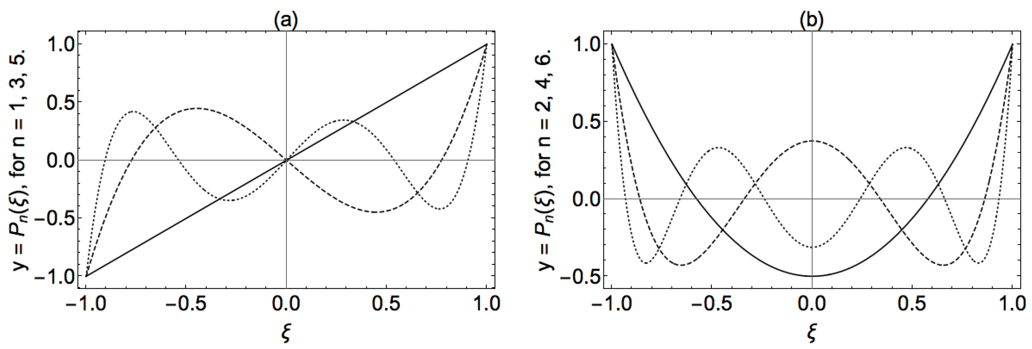
4.3. Visualization and Summary

As an example, Figure 2a,b shows how the Legendre polynomials $P_3\left(\xi \right)$ and $P_4\left(\xi \right)$ compare to Legendre functions $P_{\nu }\left(\xi \right)$ that have index values $\nu$ that are slightly smaller and larger than 3 and 4, respectively. This figure visualizes a summary of our result as follows. As we concluded from Equation (22), Legendre functions of the first kind $P_{\nu }\left(\xi \right)$ are polynomials if and only if the index $\nu$ takes an integer value. Because polynomials are bounded, Lemma 1 implies they must be either even or odd. This was Corollary 1. The symmetry of the Legendre polynomials was visualized earlier in Figure 1. In Figure 2, the Legendre polynomials $P_3\left(\xi \right)$ and $P_4\left(\xi \right)$ are represented by the dotted curves. In this figure, they are rather provided as a reference for inspection of the graphs of the other Legendre functions $P_{\nu }\left(\xi \right)$. As we proved in Section 4.2, for non-integer values of $\nu$, the functions $P_{\nu }\left(\xi \right)$ are neither odd nor even, so their graphs are non-symmetrical. Therefore, according to the Corollary 2, these functions must be unbounded at $\xi =-1$. These aspects of Legendre functions are clearly recognizable in Figure 2.

5. Conclusions

To summarize our focus and line of reasoning, we list the following observations.

In important applications in physics such as atomic physics, electro-magnetism, classical gravitation, and in astro- and geophysical fluid dynamics, particularly when Laplace’s operator is involved in spheroidal coordinates, Legendre’s Equation (3) is key.

The mathematical literature about special functions offers the extensive and detailed documentation of the general solution of this equation in terms of Legendre functions of the first and second kind.

The complete problem statement in physics, however, often does not merely consist of Legendre’s equation, but rather of Legendre’s equation supplemented with the requirement that we are looking for functions that solve this equation while they remain finite throughout the domain of application. A consequence of this condition is that all Legendre functions except Legendre polynomials are unacceptable, not as solutions of Legendre’s equation, but as solutions of the problem statement in physics.

From the point of view of physics, a theoretical treatment that includes detailed documentation of all Legendre functions is therefore at least uneconomical and risks missing quintessential arguments.

In the present manuscript, we offer an alternative in the form of an argument in as elementary terms as possible, that shows and explains why only Legendre polynomials are bounded and hence acceptable solutions to the stated problem. As a by-catch, we found that these polynomials must be either even or odd.

There seems to be added value in that our argument shows that these results are all consequences of a mirror symmetry in the physical state space, but only if and because this symmetry is combined with the signature of the regular singular points of Legendre’s equation, as it can be readily obtained from Frobenius’s theory. The fact that the signature of the regular singular points has such a decisive role in the argument is fully in accordance with the classical works of Fuchs on the class of differential equations that are now named after him.

References

1. Whittaker, E.T.; Watson, G.N. A Course of Modern Analysis; Cambridge University Press: Cambridge, UK, 1935. [Google Scholar]
2. Bateman, H. Higher Transcendental Functions; McGraw-Hill: New York, NY, USA, 1953. [Google Scholar]
3. Morse, P.M.; Feshbach, H. Methods of Theoretical Physics; McGraw-Hill: New York, NY, USA, 1953. [Google Scholar]
4. Abramowitz, M.; Stegun, I.A. Handbook of Mathematical Functions; Dover: New York, NY, USA, 1964. [Google Scholar]
5. Hochstadt, H. The Functions of Mathematical Physics; Pure and Applied Mathematics; Wiley: New York, NY, USA, 1971. [Google Scholar]
6. Fuchs, L.I. Zur Theorie der Linearen Differentialgleichungen mit veränderlichen Coefficienten. In Gesammelte Mathematische Werke von L. Fuchs; Fuchs, R., Schlesinger, L., Eds.; University Of Michigan Library: Berlin, Germany, 1865; Volume I, pp. 111–158. [Google Scholar]
7. Fuchs, L.I. Zur Theorie der Linearen Differentialgleichungen mit veränderlichen Coefficienten. J. Die Reine Angew. Math. 1866, 66, 159–204. [Google Scholar]
8. Gray, J. Linear Differential Equations and Group Theory from Riemann to Poincaré; Birkhäuser: Boston, MA, USA, 1986; ISBN 0-8176-3318-9. [Google Scholar]
9. Frobenius, F.G. Reihen. In Gesammelte Abhandlungen; Serre, J.P., Ed.; Springer: Berlin, Germany, 1968; Volume 1, pp. 84–105. [Google Scholar]
10. Boyce, W.E.; Di Prima, R.C. Elementary Differential Equations and Boundary Value Problems, 11th ed.; Wiley: Hoboken, NJ, USA, 2013; Chapter 5.6. [Google Scholar]
11. Schiff, L.I. Quantum Mechanics; McGraw-Hill: New York, NY, USA, 1955. [Google Scholar]
12. Rose, M. Elementary Theory of Angular Momentum; John Wiley & Sons: New York, NY, USA, 1957. [Google Scholar]
13. van der Toorn, R. Elementary properties of Non-Linear Rossby-Haurwitz Planetary Waves Revisited in Terms of the Underlying Spherical Symmetry. AIMS Math. 2019, 4, 279–298. [Google Scholar] [CrossRef]
14. Coddington, E.A. An Introduction to Ordinary Differential Equations; Prentice-Hall: Englewood Cliffs, NJ, USA, 1961. [Google Scholar]
15. van der Toorn, R. Tandem Recurrence Relations for Coefficients of Logarithmic Frobenius Series Solutions about Regular Singular Points. Available online: https://www.preprints.org/manuscript/202202.0289/v1 (accessed on 23 February 2022).
16. Jackson, J.D. Classical Electrodynamics; Willey: New York, NY, USA, 1962. [Google Scholar]
17. Dong, H.; Zhang, D.; Guo, Y. A Reference Ball Based Iterative Algorithm for Imaging Acoustic Obstacle from Phaseless Far-Field Data. Inverse Probl. Imaging 2019, 13, 177–195. [Google Scholar] [CrossRef] [Green Version]
18. Van der Toorn, R.; Zimmerman, J.T.F. On the Spherical Approximation of the Geopotential in Geophysical Fluid Dynamics and the Use of a Spherical Coordinate System. J. Geophys. Astrophys. Fluid Dyn. 2008, 102, 349–371. [Google Scholar] [CrossRef]
19. Butkov, E. Mathematical Physics; Addison-Wesley Publishing Company: Boston, MA, USA, 1968. [Google Scholar]
20. Wolfram Research Inc. Mathematica; Version 12.2; Wolfram Research Inc.: Champaign, IL, USA, 2020. [Google Scholar]
21. Forsyth, A.R. A Treatise on Differential Equations; MacMillan: New York, NY, USA, 1903. [Google Scholar]
22. Ince, E. Ordinary Differential Equations; Longmans, Green and Co. Ltd.: London, UK, 1927. [Google Scholar]
23. Goode, S.; Annin, S. Differential Equations and Linear Algebra; Pearson: London, UK, 2014. [Google Scholar]
Figure 1. This figure illustrates Corollary 1: (a) the Legendre polynomials of odd index value are centrally symmetric with respect to the origin of the ( ξ , y ) plane. This is illustrated here for index values 1 (solid), 3 (dashed) and 5 (dotted); and (b) the Legendre polynomials P n ( ξ ) that have an even index n are mirror symmetric with respect to the vertical axis of the ( ξ , y ) plane. This is illustrated here for index values 2 (solid), 4 (dashed) and 6 (dotted).
Symmetry 14 00741 g001
Figure 2. This figure illustrates our main results: (a) Legendre functions of the first kind P ν ( ξ ) are plotted for index values 11 / 4 (solid), 12 / 4 (dotted) and 13 / 4 (dashed); and (b) Legendre functions of the first kind P ν ( ξ ) are plotted for index values 15 / 4 (solid), 16 / 4 (dotted) and 17 / 4 (dashed) [20]. Because 12 / 4 = 3 and 16 / 4 = 4 are integers, the dotted curves represent polynomials which are bounded and must hence be symmetrical according to Corollary 1. The other curves are not symmetrical; hence, they must represent functions that are unbounded at ξ = 1 according to Corollary 2. The fact that P ν ( ξ ) is neither even nor odd if ν is not an integer was proven in Section 4.2.
Symmetry 14 00741 g002