Stability Switching Curves and Hopf Bifurcation of a Fractional Predator–Prey System with Two Nonidentical Delays

Abstract

In this paper, we propose and analyze a three-dimensional fractional predator–prey system with two nonidentical delays. By choosing two delays as the bifurcation parameter, we first calculate the stability switching curves in the delay plane. By judging the direction of the characteristic root across the imaginary axis in stability switching curves, we obtain that the stability of the system changes when two delays cross the stability switching curves, and then, the system appears to have bifurcating periodic solutions near the positive equilibrium, which implies that the trajectory of the system is the axial symmetry. Secondly, we obtain the conditions for the existence of Hopf bifurcation. Finally, we give one example to verify the correctness of the theoretical analysis. In particular, the geometric stability switch criteria are applied to the stability analysis of the fractional differential predator–prey system with two delays for the first time.

1. Introduction

Time delays are a common phenomenon in biological models because biological activity is not an instantaneous process, such as the gestation period, the hunting delay of the predator to the prey, and the delay of the predator and prey maturation. For simplicity, small and insignificant delays are frequently ignored in modeling or assume that delay does not affect the dynamic behavior of the system [1,2,3,4]. However, this hypothesis is unreasonable when delay is a vital factor of system stability. In [5], a predator–prey system with maturation and gestation delay was proposed, and the authors discovered that the increase of delay caused a stable system to become unstable, and even the phenomenon of stable switching appeared. Specifically, Hu [6] proposed the following Lotka–Volterra predator–prey system with multiple delays:

$$\begin{array}{cc}\hfill & \frac{dx\left(t\right)}{dt}=x\left(t\right)[r_1-a_{11}x(t-\tau )-a_{12}y(t-{\tau }_1)],\hfill \\ \hfill & \frac{dy\left(t\right)}{dt}=y\left(t\right)[-r_2+a_{21}x(t-{\tau }_2)-a_{22}y(t-\tau )],\hfill \end{array}$$

(1)

where $x\left(t\right)$ and $y\left(t\right)$ denote the densities of the prey and predator population at time t. $r_1$ is the growth rate of the prey. $r_2$ denotes the death rate of the predators. $a_{11}$ and $a_{22}$ are the crowding rates of the prey and predator, respectively. $a_{12}$ is the rate of predation. $a_{21}$ stands for the rate of conversion. $\tau$ is the gestation period of the prey and predator. ${\tau }_1$ denotes the hunting delay of the predator to the prey. ${\tau }_2$ is the delay of the predator maturation. The authors assumed that the sum of ${\tau }_1$ and ${\tau }_2$ is equal to $\tau$.

Because fractional calculus can describe the memory properties of the system, it has attracted extensive attention of many researchers [7]. Mandelbrot [8] first proposed the existence of many fractional-order phenomena in nature and engineering applications. Compared with the integer order, the fractional order can more accurately reflect the dynamic behavior of the real system [9]. Fractional differential equations have become one of the important tools in many disciplines and engineering fields. The are applied in neural networks [10,11], medical studies [12,13,14], and biology [15] to simulate various physical phenomena and biological processes. Many scholars have introduced fractional calculus to the predator–prey system [16,17,18].

In addition, many scholars have considered the influence of delay on the stability and existence of the Hopf bifurcation of fractional-order systems. In [19], the authors investigated a fractional-order BAM neural network involving leakage delay, and they showed that the stability of the system changes because of the introduction of the time delay. In [20], the stability and Hopf bifurcation of a fractional predator–prey system with the Holling type II function response were studied, and the author discovered that Hopf bifurcation occurs when delay crosses some critical values. With the increasing of the number of delays, complex and even new dynamic phenomena will appear. Huang [21] studied the effect of extended delayed feedback on the fractional predator–prey model, and the results demonstrated that the Hopf bifurcation of the system can be effectively controlled by adjusting the extended delayed feedback and fractional order. In [22], for a fractional predator–prey model with two nonidentical delays, an appropriate time delay can be chosen to delay the start of bifurcation. Xu [23,24,25] studied neural network models with two delays. The stability of these models was studied by fixing one delay and choosing the other delay as a bifurcation parameter, then critical values for Hopf bifurcation were obtained.

In [26], the authors studied the global stability of the equilibrium of a three-dimensional competitive Lotka–Volterra system. However, the time delay was not considered in this model. As far we know, the effect of the time delay on the system dynamics is inevitable, such as gestation delay, maturation delay, and hunting delay. Thus, based on [6,26], combining the fractional-order derivative with the time delay, we considered the following fractional-order predator–prey model with two delays:

$$\begin{array}{cc}\hfill & D^q{x}_1\left(t\right)=x_1\left(t\right)[b_1-a_{11}{x}_1(t-{\tau }_1)-a_{12}{x}_2(t-{\tau }_2)-a_{13}{x}_3(t-{\tau }_2)],\hfill \\ \hfill & D^q{x}_2\left(t\right)=x_2\left(t\right)[-b_2+a_{21}{x}_1(t-{\tau }_1)-a_{22}{x}_2\left(t\right)],\hfill \\ \hfill & D^q{x}_3\left(t\right)=x_3\left(t\right)[-b_3+a_{31}{x}_1(t-{\tau }_1)-a_{33}{x}_3\left(t\right)],\hfill \end{array}$$

(2)

where the derivative is the Caputo fractional derivative and $q\in (0,1]$. $x_1\left(t\right)$ is the density of the prey. $x_2\left(t\right)$ and $x_3\left(t\right)$ denote the population densities of two different predators at time t, respectively. $b_1$ denotes the growth rate of the prey. $b_2$ and $b_3$ represent the death rate of the first predator and the second predator, respectively. The crowding rate of the second predator is represented by $a_{33}$. $a_{13}$ and $a_{31}$ are the capture rate and conversion rate of the second predator, respectively. ${\tau }_1,{\tau }_2,a_{11},a_{12},a_{21}$, and $a_{22}$ are the same as those in System (1). The initial conditions for System (2) are $x_1\left(0\right)={\phi }_1,x_2\left(0\right)={\phi }_2,x_3\left(0\right)={\phi }_3$, and ${\phi }_i>0(i=1,2,3)$.

Generally, the stability of the model with two delays is studied by fixing one delay and choosing the other delay as a bifurcation parameter. For example, by calculating the crossing curve and the direction of stability change, Gu [27] obtained the stability of a two-delay system by the geometric method. In this paper, we took the method of the stable switching curve in the literature [28] to study the stability and the existence of the Hopf bifurcation of the system. However, the method can only deal with the characteristic equations of the following special form, that is $D(\lambda ,{\tau }_1,{\tau }_2)=P_0\left(\lambda \right)+P_1\left(\lambda \right)e^{-\lambda {\tau }_1}+P_2\left(\lambda \right)e^{-\lambda {\tau }_2}+P_3\left(\lambda \right)e^{-\lambda ({\tau }_1+{\tau }_2)}=0$. In particular, if the coefficients of the characteristic equation depend on the time delay, the method of the stable switching curve in the literature [28] is invalid. Matsumoto [29] considered the stability of the integer-order Lotka–Volterra competition model with two delays by applying the method in [28], and it was indicated that the positive equilibrium is stable in the region including the origin and being surrounded by stability switching curves. A method to determine the stability region of a differential equation with two delays was studied [30], and it was shown that the small change of delay will lead to an obvious change of the size and shape of the stability region. Reference [31] proposed the method of stability analysis for models with two delays and delay-dependent parameters. The stability switching curves was obtained in the feasible region, and according to the direction of crossing, the stability of the system on both sides of the curve was determined.

Based on the method of [28] and System (2), in this paper, we studied the fractional-order predator–prey model with two delays. By choosing two delays as the bifurcation parameter, we calculated the stability switching curves of System (2) and the direction of stability change, so as to investigate the local stability and the existence of the Hopf bifurcation of the system. As far as we know, the fractional-order differential models with two delays considering the simultaneous change of two delays is not found in the existing literature. Although [22,32,33] studied the stability and Hopf bifurcation for fractional-order systems with two delays, in these works, usually, one delay was fixed and another delay selected as the bifurcation parameter. However, in this paper, by taking two delays as the bifurcation parameter simultaneously, we discuss the stability of the fractional differential equation and the existence of Hopf bifurcation. Compared with the literature [26], an integer-order predator–prey model without delay was studied. In our paper, we considered the stability and Hopf bifurcation of the fractional-order predator–prey model with two delays. When the delay equals zero and the fractional order $q=1$, our model degenerated into the described model in the literature [26]. Our model is more general.

This paper is organized as follows. In Section 2, we calculate the stability switching curves. Next, using the stability switching curve methods, we obtain that the stability of the system changes when two delays cross the stability switching curves, and then, the system appears to have bifurcating periodic solutions near the positive equilibrium. In Section 3, we discuss the existence of the Hopf bifurcation of System (2). It is shown that the trajectory of the system is the axial symmetry. In Section 4, the theoretical findings are validated by numerical simulations. In Section 5, we give a brief summary of this paper.

2. Stability Analysis

In this section, we first calculate the characteristic equation of the positive equilibrium of System (2) and give some basic assumptions. Next, we derive the concrete expression of the stability switching curves. Finally, the direction of the characteristic roots through the imaginary axis is discussed.

2.1. Local Stability Analysis of the Positive Equilibrium

Now, we study the local stability analysis of the positive equilibrium of System (2) and give some basic assumptions. Based on [1], the following two definitions are given.

Definition 1.

The Caputo fractional-order derivative is defined by:

$$D^{q}f\left(t\right)=\frac{1}{\mathsf{\Gamma }(l-q)}{\int }_0^t{(t-s)}^{l-q-1}{f}^{\left(l\right)}\left(s\right)dt,$$

where $l-1<q\le l\in {\mathcal{Z}}^{+}$, $\mathsf{\Gamma }(·)$ is the Gamma function, and $\mathsf{\Gamma }\left(s\right)={\int }_0^{\infty }{t}^{s-1}{e}^{-t}dt$. Based on the Laplace transform, we can express the following:

$$L\{D^{q}f\left(t\right);s\}=s^{q}F\left(s\right)-\sum _{k=0}^{l-1}{s}^{q-k-1}{f}^{\left(k\right)}\left(0\right),l-1<q\le l\in {\mathcal{Z}}^{+}.$$

If $f^{\left(k\right)}\left(0\right)=0.k=1,2,\cdots ,n$, then $L\{D^{q}f\left(t\right);s\}=s^{q}F\left(s\right)$.

Definition 2.

Consider the following system:

$$D^q{x}_i\left(t\right)=f_i\left(x_i\left(t\right)\right),i=1,2,\cdots ,n,$$

(3)

where $x_i\left(t\right)=(x_1\left(t\right),x_2\left(t\right)\cdots ,x_n\left(t\right)),f_i\left(t\right)=(f_1\left(t\right),f_2\left(t\right)\cdots ,f_n\left(t\right))$. The equilibrium of System (3) is defined by $f_i\left(x_i^{\ast }\right)=0$, and the equilibrium can be obtained $(x_1^{\ast },x_2^{\ast },\cdots ,x_n^{\ast })$.

According to Definition 2, if $\left(H_1\right)$:$D_2>0$, $D_3>0$, System (2) has a unique positive equilibrium:

$$E^{\ast }(x_1,x_2,x_3)=(\frac{D_1}{D},\frac{D_2}{D},\frac{D_3}{D}),$$

where $D=a_{11}{a}_{22}{a}_{33}+a_{12}{a}_{21}{a}_{33}+a_{22}{a}_{31}{a}_{13},D_1=a_{22}{a}_{33}{b}_1+a_{13}{a}_{22}{b}_3+a_{12}{a}_{33}{b}_2,D_2=a_{33}{a}_{21}{b}_1-(a_{11}{a}_{33}+a_{13}{a}_{31})b_2+a_{21}{a}_{31}{b}_3,D_3=a_{22}{a}_{31}{b}_1+a_{12}{a}_{31}{b}_2-(a_{11}{a}_{22}+a_{12}{a}_{21})b_3.$

The corresponding characteristic equation of System (2) at $E^{\ast }$ is:

$$D(\lambda ,{\tau }_1,{\tau }_2)=P_0\left(\lambda \right)+P_1\left(\lambda \right)e^{-\lambda {\tau }_1}+P_2\left(\lambda \right)e^{-\lambda ({\tau }_1+{\tau }_2)}=0,$$

(4)

where $P_0\left(\lambda \right)={\lambda }^{3q}+L_1{\lambda }^{2q}+L_2{\lambda }^q,P_1\left(\lambda \right)=M_1{\lambda }^{2q}+M_2{\lambda }^q+M_3,P_2\left(\lambda \right)=S_1{\lambda }^q+S_2,$$L_1=a_{22}{x}_2+a_{33}{x}_3,L_2=a_{22}{a}_{33}{x}_2{x}_3,M_1=a_{11}{x}_1,M_2=a_{11}{a}_{22}{x}_1{x}_2+a_{11}{a}_{33}{x}_1{x}_3,M_3=a_{11}{a}_{22}{a}_{33}{x}_1{x}_2{x}_3,S_1=a_{31}{a}_{13}{x}_1{x}_3+a_{12}{a}_{21}{x}_1{x}_2,S_2=(a_{31}{a}_{13}{a}_{22}+a_{21}{a}_{12}{a}_{33})x_1{x}_2{x}_3.$

Some basic assumptions are needed so that Equation (4) is the characteristic equation of System (2):

(i)

Finite number of characteristic roots on ${\mathcal{C}}_{+}:=\{\lambda \in \mathcal{C}:Re\lambda >0\}$ under the condition:

$$deg\left(P_0\left(\lambda \right)\right)\ge max\{deg\left(P_1\left(\lambda \right)\right),deg\left(P_2\left(\lambda \right)\right)\};$$

(ii)

Zero frequency: $\lambda$ = 0 is not a characteristic root for any ${\tau }_1$ and ${\tau }_2$, i.e.,

$$P_0\left(0\right)+P_1\left(0\right)+P_2\left(0\right)\ne 0;$$

(iii)

The polynomials $P_0$, $P_1$ and $P_2$ have no common zeros, i.e., $P_0$, $P_1$, and $P_2$ are coprime polynomials;

(iv)

$P_k^{,}s$ satisfy:

$$\underset{\lambda \to \infty }{lim}\left(\left|\frac{P_1\left(\lambda \right)}{P_0\left(\lambda \right)}\right|+\left|\frac{P_2\left(\lambda \right)}{P_0\left(\lambda \right)}\right|\right)<1.$$

Next, we verify that Equation (4) satisfies the above assumptions. For $P_0$, $P_1$, $P_2$, (i) is automatically satisfied. For $P_0\left(0\right)+P_1\left(0\right)+P_2\left(0\right)=M_3+S_2=a_{11}{a}_{22}{a}_{33}{x}_1{x}_2{x}_3+(a_{31}{a}_{13}{a}_{22}+a_{21}{a}_{12}{a}_{33})x_1{x}_2{x}_3\ne 0$, (ii) is satisfied. From the division algorithm, when $S_1\ne 0$, $M_3-\frac{S_2}{S_1}(M_2-\frac{S_2}{S_1})\ne 0$, we know the polynomials $P_0,P_1,P_2$ have no common zeros, and (iii) is satisfied.

$$\underset{\lambda \to \infty }{lim}\left(\left|\frac{M_1{\lambda }^{2q}+M_2{\lambda }^q+M_3}{{\lambda }^{3q}+L_1{\lambda }^{2q}+L_2{\lambda }^q}\right|+\left|\frac{S_1{\lambda }^q+S_2}{{\lambda }^{3q}+L_1{\lambda }^{2q}+L_2{\lambda }^q}\right|\right)=0<1,$$

(iv) holds.

As we all know, the stability of the system is determined by the distribution of the characteristic roots on the complex plane. When ${\tau }_1={\tau }_2=0$, Equation (4) becomes:

$${\lambda }^{3q}+(L_1+M_1){\lambda }^{2q}+(L_2+M_2+S_1){\lambda }^q+M_3+S_2=0.$$

(5)

Based on [34], we have the following Lemma 1.

Lemma 1.

The linear fractional-order system $D^{q}x\left(t\right)=Ax$ is asymptotically stable in the Lyapunov sense if and only if all the eigenvalues ${\lambda }_i$ of A satisfy $\left|arg\left({\lambda }_i\right)\right|>\frac{q\pi }{2}$, where A $\in {\mathcal{R}}^{n\times n}$, $q\in (0,1]$.

According to the Routh–Hurwitz criteria and Lemma 1, we obtain the following theorem.

Theorem 1.

For ${\tau }_1={\tau }_2=0$, if $\left(H_1\right)$ and

$\left(H_2\right):(L_1+M_1)(L_2+M_2+S_1)-(M_3+S_2)>0$ hold, then the positive equilibrium $E^{\ast }$ of System (2) is asymptotically stable.

2.2. Stability Switching Curves

In this subsection, the case of ${\tau }_1>0,{\tau }_2>0$, and ${\tau }_1\ne {\tau }_2$ is discussed by applying the method in [28]. We give a mathematical formula for the stability switching curves of System (2).

Assume that $\lambda =\omega (cos\frac{\pi }{2}+isin\frac{\pi }{2})(\omega >0)$ is a pure imaginary root of Equation (4). Substituting it into Equation (4), we obtain:

$$P_0\left(i\omega \right)+P_1\left(i\omega \right)e^{-i\omega {\tau }_1}+P_2\left(i\omega \right)e^{-i\omega ({\tau }_1+{\tau }_2)}=0.$$

(6)

Since $\left|e^{-i\omega {\tau }_2}\right|=1$, we have:

$$|P_0+P_1{e}^{-i\omega {\tau }_1}|=\left|P_2{e}^{-i\omega {\tau }_1}\right|,$$

(7)

which is equivalent to:

$$(P_0+P_1{e}^{-i\omega {\tau }_1})(\overline{P_0}+\overline{P_1}{e}^{i\omega {\tau }_1})=P_2{e}^{-i\omega {\tau }_1}\left(\overline{P_2}{e}^{i\omega {\tau }_1}\right).$$

A simple calculation gives that:

$${\left|P_0\right|}^2+{\left|P_1\right|}^2+2Re\left(P_0\overline{P_1}\right)cos\left(\omega {\tau }_1\right)-2Im\left(P_0\overline{P_1}\right)sin\left(\omega {\tau }_1\right)={\left|P_2\right|}^2,$$

then:

$${\left|P_0\right|}^2+{\left|P_1\right|}^2-{\left|P_2\right|}^2=2A_{1}cos\omega {\tau }_1-2B_{1}sin\omega {\tau }_1,$$

(8)

where:

$$\begin{array}{cc}\hfill A_1& =Re(-P_0\overline{P_1})\hfill \\ \hfill & =-[M_1{\omega }^{5q}+(M_1{L}_2+M_2{L}_1){\omega }^{3q}+M_3{L}_2{\omega }^q]cos\frac{q\pi }{2}\hfill \\ \hfill & -(M_2{\omega }^{4q}+M_3{L}_1{\omega }^{2q})cosq\pi +M_3{\omega }^{3q}cos\frac{3q\pi }{2}\hfill \\ \hfill & -M_1{L}_1{\omega }^{4q}+M_2{L}_2{\omega }^{2q},\hfill \end{array}$$

$$\begin{array}{cc}\hfill B_1& =Im(-P_0\overline{P_1})\hfill \\ \hfill & =-[M_1{\omega }^{5q}+(M_2{L}_1-M_1{L}_2){\omega }^{3q}+M_3{L}_2{\omega }^q]sin\frac{q\pi }{2}\hfill \\ \hfill & -(M_2{\omega }^{4q}+M_3{L}_1{\omega }^{2q})sinq\pi -M_3{\omega }^{3q}sin\frac{3q\pi }{2}.\hfill \end{array}$$

Let ${\varphi }_1\left(\omega \right)=arg(-P_0\overline{P_1})$, then:

$$A_1=\sqrt{A_1^2+B_1^2}cos\left({\varphi }_1\left(\omega \right)\right),$$

$$B_1=\sqrt{A_1^2+B_1^2}sin\left({\varphi }_1\left(\omega \right)\right).$$

Equation (8) becomes:

$${\left|P_0\right|}^2+{\left|P_1\right|}^2-{\left|P_2\right|}^2=2\sqrt{A_1^2+B_1^2}cos({\varphi }_1\left(\omega \right)+\omega {\tau }_1).$$

(9)

Obviously, a sufficient and necessary condition for the existence of ${\tau }_1\in {\mathcal{R}}^{+}$ satisfying the Equation (9) is:

$${\left|P_0\right|}^2+{\left|P_1\right|}^2-{\left|P_2\right|}^2\le 2\sqrt{A_1^2+B_1^2}.$$

(10)

Define:

$$\begin{array}{cc}\hfill F\left(\omega \right)& ={({\left|P_0\right|}^2+{\left|P_1\right|}^2-{\left|P_2\right|}^2)}^2-4(A_1^2+B_1^2)\hfill \\ \hfill & ={\{{\omega }^{6q}+G_1{\omega }^{5q}+G_2{\omega }^{4q}+G_3{\omega }^{3q}+G_4{\omega }^{2q}+G_5{\omega }^q+G_6\}}^2-4(A_1^2+B_1^2),\hfill \end{array}$$

where $G_1=2L_{1}cos\frac{q\pi }{2},G_2=L_1^2+M_1^2+2L_{2}cosq\pi ,G_3=2(L_1{L}_2+M_1{M}_2)cos\frac{q\pi }{2},G_4=(L_2^2+M_2^2-S_1^2)+2M_1{M}_{2}cosq\pi ,G_5=2(M_2{M}_3-S_1{S}_2)cos\frac{q\pi }{2},G_6=M_3^2-S_2^2.$

The inequality (10) is equivalent such that there is a crossing set $\mathsf{\Omega }$ for $\omega \in {\mathcal{R}}^{+}$ in which $F\left(\omega \right)\le 0$, and $\mathsf{\Omega }$ consists of a finite number of intervals of finite length. Let ${\varphi }_1\left(\omega \right)+\omega {\tau }_1={\psi }_1\left(\omega \right)$; we have:

$$cos\left({\psi }_1\left(\omega \right)\right)=\frac{{\left|P_0\right|}^2+{\left|P_1\right|}^2-{\left|P_2\right|}^2}{2\sqrt{A_1^2+B_1^2}},{\psi }_1\in [0,\pi ],$$

then:

$${\tau }_{1,n_1}^{\pm }\left(\omega \right)=\frac{\pm {\psi }_1\left(\omega \right)-{\varphi }_1\left(\omega \right)+2n_1\pi }{\omega },n_1\in \mathcal{Z}.$$

(11)

The characteristic Equation (6) can be rewritten as:

$$\begin{array}{cc}\hfill e^{-i\omega {\tau }_2}& =-\frac{P_0\left(i\omega \right)+P_1\left(i\omega \right)e^{-i\omega {\tau }_1}}{P_2\left(i\omega \right)e^{-i\omega {\tau }_1}},\hfill \end{array}$$

(12)

From Equation (12), we have:

$$\begin{array}{cc}\hfill {\tau }_2& =-\frac{1}{\omega }arg\left\{-\frac{P_0\left(i\omega \right)+P_1\left(i\omega \right)e^{-i\omega {\tau }_1}}{P_2\left(i\omega \right)e^{-i\omega {\tau }_1}}\right\}+2n_2\pi ,n_2\in \mathcal{Z}\hfill \\ \hfill & =-\frac{1}{\omega }arg\left\{-\frac{(P_0\left(i\omega \right)+P_1\left(i\omega \right)e^{-i\omega {\tau }_1})\overline{P_2\left(i\omega \right)e^{-i\omega {\tau }_1}}}{{\left|P_2\left(i\omega \right)\right|}^2}\right\}+2n_2\pi \hfill \\ \hfill & =-\frac{1}{\omega }arg\left\{-\frac{N_1+N_{2}i}{N}\right\}+2n_2\pi ,\hfill \end{array}$$

(13)

where:

$$\begin{array}{cc}\hfill N& =S_1^2{\omega }^{2q}+S_2^2+2S_1{S}_2{\omega }^{q}cos\frac{q\pi }{2},\hfill \end{array}$$

$$\begin{array}{cc}\hfill N_1& =S_1{\omega }^{4q}cos(q\pi +\omega {\tau }_1)+S_1{L}_1{\omega }^{3q}cos(\frac{q\pi }{2}+\omega {\tau }_1)+S_1{L}_2{\omega }^{2q}cos\omega {\tau }_1\hfill \\ \hfill & +S_1{M}_1{\omega }^{3q}cos\frac{q\pi }{2}+S_1{M}_2{\omega }^{2q}+S_1{M}_3{\omega }^{q}cos\frac{q\pi }{2}+S_2{\omega }^{3q}cos(\frac{3q\pi }{2}\hfill \\ \hfill & +\omega {\tau }_1)+S_2{L}_1{\omega }^{2q}cos(q\pi +\omega {\tau }_1)+S_2{L}_2{\omega }^{q}cos(\frac{q\pi }{2}+\omega {\tau }_1)\hfill \\ \hfill & +S_2{M}_1{\omega }^{2q}cosq\pi +S_2{M}_3+S_2{M}_2{\omega }^{q}cos\frac{q\pi }{2},\hfill \\ \hfill N_2& =S_1{\omega }^{4q}sin(q\pi +\omega {\tau }_1)+S_1{L}_1{\omega }^{3q}sin(\frac{q\pi }{2}+\omega {\tau }_1)+S_1{L}_2{\omega }^{2q}sin\omega {\tau }_1\hfill \\ \hfill & -S_1{M}_3{\omega }^{q}sin\frac{q\pi }{2}+S_2{\omega }^{3q}sin(\frac{3q\pi }{2}+\omega {\tau }_1)+S_2{L}_1{\omega }^{2q}sin(q\pi +\omega {\tau }_1)\hfill \\ \hfill & +S_2{L}_2{\omega }^{q}sin(\frac{q\pi }{2}+\omega {\tau }_1)+S_2{M}_1{\omega }^{2q}sinq\pi +S_2{M}_2{\omega }^{q}sin\frac{q\pi }{2}.\hfill \end{array}$$

(14)

Hence, we consider that ${\tau }_2$ can be regarded as a function of ${\tau }_1$. We figure out ${\tau }_1$ from Equation (9), and substituting ${\tau }_1$ into Equation (13), it is easy to calculate the value of ${\tau }_2$ with $\omega \in \mathsf{\Omega }$. According to [28], the stability switching curves are given as:

$$\mathcal{T}:=\left\{({\tau }_{1,n_1}^{\pm }\left(\omega \right),{\tau }_{2,n_2}^{\pm }\left(\omega \right))\in R_{+}^2:\omega \in \mathsf{\Omega },n_1,n_2\in Z\right\}.$$

(15)

The other way to find ${\tau }_2$ is similar to the analysis of ${\tau }_1$. Then, we have:

$${\tau }_{2,n_2}^{\pm }\left(\omega \right)=\frac{\pm {\psi }_2\left(\omega \right)-{\varphi }_2\left(\omega \right)+2n_2\pi }{\omega },n_2\in \mathcal{Z},$$

(16)

where ${\varphi }_2\left(\omega \right)=arg\left(P_1\overline{P_2}\right),cos\left({\psi }_2\left(\omega \right)\right)=\frac{{\left|P_0\right|}^2-{\left|P_1\right|}^2-{\left|P_2\right|}^2}{2\sqrt{A_2^2+B_2^2}},{\psi }_2\in [0,\pi ],$

$$\begin{array}{cc}\hfill A_2& =Re\left(P_1\overline{P_2}\right)\hfill \\ \hfill & =[S_1{M}_1{\omega }^{3q}+(S_1{M}_3+S_2{M}_2){\omega }^q]cos\frac{q\pi }{2}+S_2{M}_1{\omega }^{2q}cosq\pi \hfill \\ \hfill & +S_1{M}_2{\omega }^{2q}+S_2{M}_3,\hfill \end{array}$$

$$\begin{array}{cc}\hfill B_2& =Im\left(P_1\overline{P_2}\right)\hfill \\ \hfill & =[S_1{M}_1{\omega }^{3q}+(S_2{M}_2-S_1{M}_3){\omega }^q]sin\frac{q\pi }{2}+S_2{M}_1{\omega }^{2q}sinq\pi .\hfill \end{array}$$

Similarly, we also have:

$$A_2=\sqrt{A_2^2+B_2^2}cos\left({\varphi }_2\left(\omega \right)\right),$$

$$B_2=\sqrt{A_2^2+B_2^2}sin\left({\varphi }_2\left(\omega \right)\right).$$

Based on the above discussion, we have the following theorem.

Theorem 2.

The characteristic Equation (4) has a pair of pure imaginary roots $\pm i\omega$ for $({\tau }_1,{\tau }_2)\in \mathcal{T}$. The stability of System (2) is transformed when $({\tau }_1,{\tau }_2)$ passes through the stability switching curves $\mathcal{T}$, where $\mathcal{T}$ is denoted by Equation (15).

2.3. Crossing Directions

In this subsection, we assume that $({\tau }_1^{\ast },{\tau }_2^{\ast })\in \mathcal{T}$, then the characteristic equation has a pair of pure imaginary roots $\pm i{\omega }^{\ast }$. If $\frac{\partial D}{\partial \lambda }(i{\omega }^{\ast },{\tau }_1^{\ast },{\tau }_2^{\ast })\ne 0$, then the characteristic Equation (4) has a pair of conjugate complex roots $\lambda ({\tau }_1,{\tau }_2)=\delta ({\tau }_1,{\tau }_2)\pm i\omega ({\tau }_1,{\tau }_2)$ in some neighborhood of $({\tau }_1^{\ast },{\tau }_2^{\ast })$, such that $\delta ({\tau }_1^{\ast },{\tau }_2^{\ast })=0$ and $\omega ({\tau }_1^{\ast },{\tau }_2^{\ast })={\omega }^{\ast }$. Next, we discuss the direction of the characteristic roots crossing the imaginary axis as $({\tau }_1^{\ast },{\tau }_2^{\ast })$ passes through the curve $\mathcal{T}$ and enters the left or right region. We call the increasing direction of $\omega$ the positive direction of the curve $\mathcal{T}$. When we move along the positive direction of the curve, the right (left)-hand side is the right (left) region.

If the condition that the implicit function theorem holds, we consider that ${\tau }_1$ and ${\tau }_2$ can be regarded as a function of $\delta$ and $\omega$. Since the tangent vector of $\mathcal{T}$ along the positive direction is $\mathit{a}=(\frac{\partial {\tau }_1}{\partial \omega },\frac{\partial {\tau }_2}{\partial \omega })$, the normal vector of $\mathcal{T}$ pointing to the right region is $\mathit{b}=(\frac{\partial {\tau }_2}{\partial \omega },-\frac{\partial {\tau }_1}{\partial \omega })$, and $({\tau }_1,{\tau }_2)$ move along the direction $\mathit{c}=(\frac{\partial {\tau }_1}{\partial \delta },\frac{\partial {\tau }_2}{\partial \delta })$. We conclude that the direction of the characteristic roots crossing the imaginary axis is determined by the sign of the inner product of $\mathit{b}$ and $\mathit{c}$,

$$\delta \left(\omega \right):=\mathit{b}·\mathit{c}=\left(\frac{\partial {\tau }_2}{\partial \omega },-\frac{\partial {\tau }_1}{\partial \omega }\right)·\left(\frac{\partial {\tau }_1}{\partial \delta },\frac{\partial {\tau }_2}{\partial \delta }\right)=\frac{\partial {\tau }_1}{\partial \delta }\frac{\partial {\tau }_2}{\partial \omega }-\frac{\partial {\tau }_2}{\partial \delta }\frac{\partial {\tau }_1}{\partial \omega }=\left|\begin{array}{cc}\frac{\partial {\tau }_1}{\partial \delta }& \frac{\partial {\tau }_1}{\partial \omega }\\ \frac{\partial {\tau }_2}{\partial \delta }& \frac{\partial {\tau }_2}{\partial \omega }\end{array}\right|.$$

(17)

If $\delta \left(\omega \right)>0\left(\delta \right(\omega )<0)$, when we move along the positive direction of the stability switching curves, the characteristic equation has roots with positive real parts on the right (left)-hand region of the curve $\mathcal{T}$.

We calculate $\frac{\partial {\tau }_1}{\partial \delta }$, $\frac{\partial {\tau }_2}{\partial \delta }$, $\frac{\partial {\tau }_1}{\partial \omega }$, and $\frac{\partial {\tau }_2}{\partial \omega }$ from the characteristic equation $D(\lambda ,{\tau }_1,{\tau }_2)=0$, and we obtain:

$$\begin{array}{cc}\hfill \frac{\partial D}{\partial \delta }& =\frac{\partial D}{\partial {\tau }_1}\frac{\partial {\tau }_1}{\partial \delta }+\frac{\partial D}{\partial {\tau }_2}\frac{\partial {\tau }_2}{\partial \delta },\hfill \\ \hfill \frac{\partial D}{\partial \omega }& =\frac{\partial D}{\partial {\tau }_1}\frac{\partial {\tau }_1}{\partial \omega }+\frac{\partial D}{\partial {\tau }_2}\frac{\partial {\tau }_2}{\partial \omega }.\hfill \end{array}$$

(18)

Then, the matrix form of Equation (18) is given as:

$$\left(\frac{\partial D}{\partial {\tau }_1},\frac{\partial D}{\partial {\tau }_2}\right)\left(\begin{array}{cc}\frac{\partial {\tau }_1}{\partial \delta }& \frac{\partial {\tau }_1}{\partial \omega }\\ \frac{\partial {\tau }_2}{\partial \delta }& \frac{\partial {\tau }_2}{\partial \omega }\end{array}\right)=\left(\frac{\partial D}{\partial \delta },\frac{\partial D}{\partial \omega }\right).$$

(19)

The real and imaginary parts of $\frac{\partial D}{\partial {\tau }_1},\frac{\partial D}{\partial {\tau }_2},\frac{\partial D}{\partial \delta }$ and $\frac{\partial D}{\partial \omega }$ are denoted by $R_1,I_1,R_2,I_2,R_0,I_0,$$R,I$. Equation (19) can be rewritten as:

$$\left(\begin{array}{cc}{R}_1& R_2\\ I_1& I_2\end{array}\right)\left(\begin{array}{cc}\frac{\partial {\tau }_1}{\partial \delta }& \frac{\partial {\tau }_1}{\partial \omega }\\ \frac{\partial {\tau }_2}{\partial \delta }& \frac{\partial {\tau }_2}{\partial \omega }\end{array}\right)=\left(\begin{array}{cc}{R}_0& R\\ I_0& I\end{array}\right),$$

where:

$$\begin{array}{cc}\hfill R_0:& =\frac{\partial ReD(\lambda ,{\tau }_1,{\tau }_2)}{\partial \delta }{|}_{\lambda =i{\omega }^{\ast }}\hfill \\ \hfill & =Re\{P_0^{{}^{\prime }}\left(i{\omega }^{\ast }\right)+P_1^{{}^{\prime }}\left(i{\omega }^{\ast }\right)e^{-i{\omega }^{\ast }{\tau }_1^{\ast }}-{\tau }_1^{\ast }{P}_1\left(i{\omega }^{\ast }\right)e^{-i{\omega }^{\ast }{\tau }_1^{\ast }}\hfill \\ \hfill & +P_2^{{}^{\prime }}\left(i{\omega }^{\ast }\right)e^{-i{\omega }^{\ast }({\tau }_1^{\ast }+{\tau }_2^{\ast })}-({\tau }_1^{\ast }+{\tau }_2^{\ast })P_2\left(i{\omega }^{\ast }\right)e^{-i{\omega }^{\ast }({\tau }_1^{\ast }+{\tau }_2^{\ast })}\}\hfill \\ \hfill & =3q{{\omega }^{\ast }}^{3q-1}sin\frac{3q\pi }{2}+2L_{1}q{{\omega }^{\ast }}^{2q-1}sinq\pi +q{L}_2{{\omega }^{\ast }}^{q-1}sin\frac{q\pi }{2}\hfill \\ \hfill & +2q{M}_1{{\omega }^{\ast }}^{2q-1}sin(q\pi -{\omega }^{\ast }{\tau }_1^{\ast })+q{M}_2{{\omega }^{\ast }}^{q-1}sin(\frac{q\pi }{2}-{\omega }^{\ast }{\tau }_1^{\ast })\hfill \\ \hfill & -{\tau }_1[M_1{{\omega }^{\ast }}^{2q}cos(q\pi -{\omega }^{\ast }{\tau }_1^{\ast })+M_2{{\omega }^{\ast }}^{q}cos(\frac{q\pi }{2}-{\omega }^{\ast }{\tau }_1^{\ast })\hfill \\ \hfill & +M_{3}cos{\omega }^{\ast }{\tau }_1^{\ast }]+S_{1}q{{\omega }^{\ast }}^{q-1}sin(\frac{q\pi }{2}-{\omega }^{\ast }({\tau }_1^{\ast }+{\tau }_2^{\ast }))\hfill \\ \hfill & -({\tau }_1^{\ast }+{\tau }_2^{\ast })[S_1{{\omega }^{\ast }}^{q}cos(\frac{q\pi }{2}-{\omega }^{\ast }({\tau }_1^{\ast }+{\tau }_2^{\ast }))+S_{2}cos{\omega }^{\ast }({\tau }_1^{\ast }+{\tau }_2^{\ast })],\hfill \end{array}$$

(20)

$$\begin{array}{cc}\hfill I_0:& =\frac{\partial ImD(\lambda ,{\tau }_1,{\tau }_2)}{\partial \delta }{|}_{\lambda =i{\omega }^{\ast }}\hfill \\ \hfill & =Im\{P_0^{{}^{\prime }}\left(i{\omega }^{\ast }\right)+P_1^{{}^{\prime }}\left(i{\omega }^{\ast }\right)e^{-i{\omega }^{\ast }{\tau }_1^{\ast }}-{\tau }_1^{\ast }{P}_1\left(i{\omega }^{\ast }\right)e^{-i{\omega }^{\ast }{\tau }_1^{\ast }}\hfill \\ \hfill & +P_2^{{}^{\prime }}\left(i{\omega }^{\ast }\right)e^{-i{\omega }^{\ast }({\tau }_1^{\ast }+{\tau }_2^{\ast })}-({\tau }_1^{\ast }+{\tau }_2^{\ast })P_2\left(i{\omega }^{\ast }\right)e^{-i{\omega }^{\ast }({\tau }_1^{\ast }+{\tau }_2^{\ast })}\}\hfill \\ \hfill & =-(3q{{\omega }^{\ast }}^{3q-1}cos\frac{3q\pi }{2}+2L_{1}q{{\omega }^{\ast }}^{2q-1}cosq\pi +q{L}_2{{\omega }^{\ast }}^{q-1}cos\frac{q\pi }{2})\hfill \\ \hfill & -[2q{M}_1{{\omega }^{\ast }}^{2q-1}cos(q\pi -{\omega }^{\ast }{\tau }_1^{\ast })+q{M}_2{{\omega }^{\ast }}^{q-1}cos(\frac{q\pi }{2}-{\omega }^{\ast }{\tau }_1^{\ast })]\hfill \\ \hfill & -{\tau }_1^{\ast }[M_1{{\omega }^{\ast }}^{2q}sin(q\pi -{\omega }^{\ast }{\tau }_1^{\ast })+M_2{{\omega }^{\ast }}^{q}sin(\frac{q\pi }{2}-{\omega }^{\ast }{\tau }_1^{\ast })\hfill \\ \hfill & -M_{3}sin{\omega }^{\ast }{\tau }_1^{\ast }]-S_{1}q{{\omega }^{\ast }}^{q-1}cos(\frac{q\pi }{2}-{\omega }^{\ast }({\tau }_1^{\ast }+{\tau }_2^{\ast }))\hfill \\ \hfill & -({\tau }_1^{\ast }+{\tau }_2^{\ast })[S_1{{\omega }^{\ast }}^{q}sin(\frac{q\pi }{2}-{\omega }^{\ast }({\tau }_1^{\ast }+{\tau }_2^{\ast }))-S_{2}sin{\omega }^{\ast }({\tau }_1^{\ast }+{\tau }_2^{\ast })],\hfill \end{array}$$

(21)

$$\begin{array}{cc}\hfill R=\frac{\partial ReD(\lambda ,{\tau }_1,{\tau }_2)}{\partial \omega }{|}_{\lambda =i{\omega }^{\ast }}& =Re\{P_0^{{}^{\prime }}\left(i{\omega }^{\ast }\right)i+P_1^{{}^{\prime }}\left(i{\omega }^{\ast }\right)i{e}^{-i{\omega }^{\ast }{\tau }_1^{\ast }}\hfill \\ \hfill & -i{\tau }_1^{\ast }{P}_1\left(i{\omega }^{\ast }\right)e^{-i{\omega }^{\ast }{\tau }_1^{\ast }}+P_2^{{}^{\prime }}\left(i{\omega }^{\ast }\right)i{e}^{-i{\omega }^{\ast }({\tau }_1^{\ast }+{\tau }_2^{\ast })}\hfill \\ \hfill & -i({\tau }_1^{\ast }+{\tau }_2^{\ast })P_2\left(i{\omega }^{\ast }\right)e^{-i{\omega }^{\ast }({\tau }_1^{\ast }+{\tau }_2^{\ast })}\}\hfill \\ \hfill & =-I_0,\hfill \end{array}$$

(22)

$$\begin{array}{cc}\hfill I=\frac{\partial ImD(\lambda ,{\tau }_1,{\tau }_2)}{\partial \omega }{|}_{\lambda =i{\omega }^{\ast }}& =Im\{P_0^{{}^{\prime }}\left(i{\omega }^{\ast }\right)i+P_1^{{}^{\prime }}\left(i{\omega }^{\ast }\right)i{e}^{-i{\omega }^{\ast }{\tau }_1^{\ast }}\hfill \\ \hfill & -i{\tau }_1^{\ast }{P}_1\left(i{\omega }^{\ast }\right)e^{-i{\omega }^{\ast }{\tau }_1^{\ast }}+P_2^{{}^{\prime }}\left(i{\omega }^{\ast }\right)i{e}^{-i{\omega }^{\ast }({\tau }_1^{\ast }+{\tau }_2^{\ast })}\hfill \\ \hfill & -i({\tau }_1^{\ast }+{\tau }_2^{\ast })P_2\left(i{\omega }^{\ast }\right)e^{-i{\omega }^{\ast }({\tau }_1^{\ast }+{\tau }_2^{\ast })}\}\hfill \\ \hfill & =R_0,\hfill \end{array}$$

(23)

$$\begin{array}{cc}\hfill R_1:& =\frac{\partial ReD(\lambda ,{\tau }_1,{\tau }_2)}{\partial {\tau }_1}{|}_{\lambda =i{\omega }^{\ast }}\hfill \\ \hfill & =Re\{(-i{\omega }^{\ast })(P_1\left(i{\omega }^{\ast }\right)e^{-i{\omega }^{\ast }{\tau }_1^{\ast }}+P_2\left(i{\omega }^{\ast }\right)e^{-i{\omega }^{\ast }({\tau }_1^{\ast }+{\tau }_2^{\ast })})\}\hfill \\ \hfill & ={\omega }^{\ast }[S_1{{\omega }^{\ast }}^{q}sin(\frac{q\pi }{2}-{\omega }^{\ast }({\tau }_1^{\ast }+{\tau }_2^{\ast }))-S_{2}sin{\omega }^{\ast }({\tau }_1^{\ast }+{\tau }_2^{\ast })\hfill \\ \hfill & -M_1{{\omega }^{\ast }}^{2q}sin(q\pi -{\omega }^{\ast }{\tau }_1^{\ast })-M_2{{\omega }^{\ast }}^{q}sin(\frac{q\pi }{2}-{\omega }^{\ast }{\tau }_1^{\ast })],\hfill \end{array}$$

(24)

$$\begin{array}{cc}\hfill I_1:& =\frac{\partial ImD(\lambda ,{\tau }_1,{\tau }_2)}{\partial {\tau }_1}{|}_{\lambda =i{\omega }^{\ast }}\hfill \\ \hfill & =Im\{(-i{\omega }^{\ast })(P_1\left(i{\omega }^{\ast }\right)e^{-i{\omega }^{\ast }{\tau }_1^{\ast }}+P_2\left(i{\omega }^{\ast }\right)e^{-i{\omega }^{\ast }({\tau }_1^{\ast }+{\tau }_2^{\ast })})\}\hfill \\ \hfill & =-{\omega }^{\ast }[S_1{{\omega }^{\ast }}^{q}cos(\frac{q\pi }{2}-{\omega }^{\ast }({\tau }_1^{\ast }+{\tau }_2^{\ast }))+S_{2}cos{\omega }^{\ast }({\tau }_1^{\ast }+{\tau }_2^{\ast })\hfill \\ \hfill & +M_1{{\omega }^{\ast }}^{2q}cos(q\pi -{\omega }^{\ast }{\tau }_1^{\ast })+M_2{{\omega }^{\ast }}^{q}cos(\frac{q\pi }{2}-{\omega }^{\ast }{\tau }_1^{\ast })],\hfill \end{array}$$

(25)

$$\begin{array}{cc}\hfill R_2:& =\frac{\partial ReD(\lambda ,{\tau }_1,{\tau }_2)}{\partial {\tau }_2}{|}_{\lambda =i{\omega }^{\ast }}\hfill \\ \hfill & =Re\{(-i{\omega }^{\ast })P_2\left(i{\omega }^{\ast }\right)e^{-i{\omega }^{\ast }({\tau }_1^{\ast }+{\tau }_2^{\ast })}\}\hfill \\ \hfill & ={\omega }^{\ast }\left[S_1{{\omega }^{\ast }}^{q}sin(\frac{q\pi }{2}-{\omega }^{\ast }({\tau }_1^{\ast }+{\tau }_2^{\ast }))-S_{2}sin{\omega }^{\ast }({\tau }_1^{\ast }+{\tau }_2^{\ast })\right],\hfill \end{array}$$

(26)

$$\begin{array}{cc}\hfill I_2:& =\frac{\partial ImD(\lambda ,{\tau }_1,{\tau }_2)}{\partial {\tau }_2}{|}_{\lambda =i{\omega }^{\ast }}\hfill \\ \hfill & =Im\{(-i{\omega }^{\ast })P_2\left(i{\omega }^{\ast }\right)e^{-i{\omega }^{\ast }({\tau }_1^{\ast }+{\tau }_2^{\ast })}\}\hfill \\ \hfill & =-{\omega }^{\ast }\left[S_1{{\omega }^{\ast }}^{q}cos(\frac{q\pi }{2}-{\omega }^{\ast }({\tau }_1^{\ast }+{\tau }_2^{\ast }))+S_{2}cos{\omega }^{\ast }({\tau }_1^{\ast }+{\tau }_2^{\ast })\right].\hfill \end{array}$$

(27)

For the computation details of $R_i$ and $I_i$$(i=0,1,2)$, see Appendix A. We consider that ${\tau }_1$ and ${\tau }_2$ can be regarded as a function of $\delta$ and $\omega$, then the following assumption is necessary:

$\left(H_3\right)$: $det\left(\begin{array}{cc}{R}_1& R_2\\ I_1& I_2\end{array}\right)=R_1{I}_2-R_2{I}_1\ne 0.$

By using the implicit function theory and $\left(H_3\right)$, we have:

$$▵\left(\omega \right):=\left(\begin{array}{cc}\frac{\partial {\tau }_1}{\partial \delta }& \frac{\partial {\tau }_1}{\partial \omega }\\ \frac{\partial {\tau }_2}{\partial \delta }& \frac{\partial {\tau }_2}{\partial \omega }\end{array}\right){|}_{\delta =0,\omega \in \mathsf{\Omega }}={\left(\begin{array}{cc}{R}_1& R_2\\ I_1& I_2\end{array}\right)}^{-1}\left(\begin{array}{cc}{R}_0& -I_0\\ I_0& R_0\end{array}\right).$$

(28)

Clearly, we obtain:

$$\delta \left(\omega \right)=det(▵\left(\omega \right))=det{\left(\begin{array}{cc}{R}_1& R_2\\ I_1& I_2\end{array}\right)}^{-1}det\left(\begin{array}{cc}{R}_0& -I_0\\ I_0& R_0\end{array}\right).$$

From $R_0^2+I_0^2\ge 0$, we know that $\delta \left(\omega \right)$ and $R_1{I}_2-R_2{I}_1$ have the same sign, that is:

$$sign\left(\delta \left(\omega \right)\right)=sign\{R_1{I}_2-R_2{I}_1\}.$$

(29)

It is easy to calculate $R_1{I}_2-R_2{I}_1=\pm {{\omega }^{\ast }}^2|-P_0\overline{P_1}|sin\left({\psi }_1\left({\omega }^{\ast }\right)\right).$ The details of the computations of $R_1{I}_2-R_2{I}_1$ are shown in Appendix B. Thus, we have the following Theorem 3.

Theorem 3.

Assume $R_1{I}_2-R_2{I}_1\ne 0$, $sign\left(\delta \right(\omega \left)\right)>0\left(sign\right(\delta \left(\omega \right))<0)$, then a pair of pure imaginary roots of the characteristic equation $D(\lambda ,{\tau }_1,{\tau }_2)=0$ cross the imaginary axis from left to right, as $({\tau }_1,{\tau }_2)$ passes through the stability switching curves from the left (right) region to the right (left) region.

3. Hopf Bifurcation

In this section, we derive the conditions for the existence of Hopf bifurcation. Based on Section 2.2, we know that the characteristic Equation (4) has a pair of pure imaginary roots on the stability switching curves.

Let us take the derivative of both sides of $D(\lambda ,{\tau }_1,{\tau }_2)=0$ with respect to ${\tau }_1$, and ${\tau }_2$ can be expressed as a function of ${\tau }_1$,

$$\begin{array}{cc}\hfill & P_0^{{}^{\prime }}\left(\lambda \right)\frac{d\lambda }{d{\tau }_1}+P_1^{{}^{\prime }}\left(\lambda \right)\frac{d\lambda }{d{\tau }_1}{e}^{-\lambda {\tau }_1}-P_1\left(\lambda \right)e^{-\lambda {\tau }_1}\left(\frac{d\lambda }{d{\tau }_1}{\tau }_1+\lambda \right)+P_2^{{}^{\prime }}\left(\lambda \right)\frac{d\lambda }{d{\tau }_1}{e}^{-\lambda ({\tau }_1+{\tau }_2)}\hfill \\ \hfill & -P_2\left(\lambda \right)e^{-\lambda ({\tau }_1+{\tau }_2)}\left[\frac{d\lambda }{d{\tau }_1}({\tau }_1+{\tau }_2)+\lambda \left(1+\frac{d{\tau }_2}{d{\tau }_1}\right)\right]=0.\hfill \end{array}$$

Thus, we have:

$$\begin{array}{cc}\hfill Re\left[\frac{d\lambda }{d{\tau }_1}\right]{|}_{\lambda =i{\omega }^{\ast }}& =Re\left\{-\frac{R_1+I_{1}i+(R_2+I_{2}i)\frac{d{\tau }_2}{d{\tau }_1}}{R_0+I_{0}i}\right\}\hfill \\ \hfill & =-\frac{R_1{R}_0+I_1{I}_0+(R_2{R}_0+I_2{I}_0)\frac{d{\tau }_2}{d{\tau }_1}}{R_0^2+I_0^2}.\hfill \end{array}$$

$$\frac{d{\tau }_2}{d{\tau }_1}=\left\{\begin{array}{cc}-\frac{N_2^{{}^{\prime }}{N}_1-N_2{N}_1^{{}^{\prime }}}{\omega (N_1^2+N_2^2)},\hfill & N_1\ne 0,\hfill \\ 0,\hfill & N_1=0,\hfill \end{array}\right.$$

where the details of the computations of $Re\left[\frac{d\lambda }{d{\tau }_1}\right]{|}_{\lambda =i{\omega }^{\ast }}$ and $\frac{d{\tau }_2}{d{\tau }_1}$ are in Appendix C. Based on the above discussions, the transversality conditions of System (2) are given as:

$\left(H_4\right)$: $R_1{R}_0+I_1{I}_0-(R_2{R}_0+I_2{I}_0)\frac{N_2^{{}^{\prime }}{N}_1-N_2{N}_1^{{}^{\prime }}}{{\omega }^{\ast }(N_1^2+N_2^2)}\ne 0.$

$\left(H_5\right)$: $R_1{R}_0+I_1{I}_0\ne 0$.

Then, we have the following conclusion:

Theorem 4.

If Conditions $\left(H_1\right)-\left(H_4\right)$ or Conditions $\left(H_1\right)-\left(H_3\right)$ and $\left(H_5\right)$ hold, then System (2) undergoes Hopf bifurcations at $E^{\ast }$ when $({\tau }_1,{\tau }_2)$ passes through the stability switching curves $\mathcal{T}$, where $\mathcal{T}=({\tau }_1^{\pm },{\tau }_2^{\pm })$ is given by Equation (15).

4. Numerical Simulation

Considering the following system:

$$\begin{array}{cc}\hfill D^q{x}_1\left(t\right)& =x_1\left(t\right)[2-\frac{1}{3}{x}_1(t-{\tau }_1)-x_2(t-{\tau }_2)-2x_3(t-{\tau }_2)],\hfill \\ \hfill D^q{x}_2\left(t\right)& =x_2\left(t\right)[-\frac{1}{3}-x_1(t-{\tau }_1)-2x_2\left(t\right)],\hfill \\ \hfill D^q{x}_3\left(t\right)& =x_3\left(t\right)[-\frac{1}{3}-x_1(t-{\tau }_1)-2x_3\left(t\right)],\hfill \end{array}$$

(30)

where $q=0.84$; we have $D_2=3.778>0$, $D_3=3.778>0$, then $\left(H_1\right)$ is satisfied. Therefore, System (30) has a unique positive equilibrium $E^{\ast }$= (1.3636,0.5152,0.5152). The characteristic equation of System (30) at $E^{\ast }$ is:

$${\lambda }^{3q}+L_1{\lambda }^{2q}+L_2{\lambda }^q+(M_1{\lambda }^{2q}+M_2{\lambda }^q+M_3)e^{-\lambda {\tau }_1}+(S_1{\lambda }^q+S_2)e^{-\lambda ({\tau }_1+{\tau }_2)}=0.$$

(31)

From Equation (4), we calculate $L_1=2.0606,L_2=1.0615,M_1=0.4545,$ $M_2=0.9366,M_3=0.4852,S_1=2.1074$, and $S_2=2.1713.$ Next, we verify the conditions that the characteristic equation $P_0\left(0\right)+P_1\left(0\right)+P_2\left(0\right)=M_3+S_2=2.6538\ne 0$, $M_3-\frac{S_2}{S_1}(M_2-\frac{S_2}{S_1})=0.5790\ne 0$. Thus, we have that some basic assumptions (i)–(iv) in Section 2 hold.

When ${\tau }_1={\tau }_2=0$, we obtain $(L_1+M_1)(L_2+M_2+S_1)-(M_3+S_2)=7.6724>0$, $\left(H_2\right)$ also holds. Then, $E^{\ast }$ is locally asymptotically stable from Theorem 1 (see Figure 1).

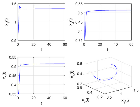
Figure 1. $E^{\ast }$ of System (30) is locally asymptotically stable when ${\tau }_1={\tau }_2=0$.

When ${\tau }_1>0$, ${\tau }_2>0$, from the definition of $F\left(\omega \right)$, we have:

$$\begin{array}{cc}\hfill F\left(\omega \right)& ={\omega }^{12q}+2.0498{\omega }^{11q}+5.4085{\omega }^{10q}+6.2190{\omega }^{9q}-1.7940{\omega }^{8q}-9.7208{\omega }^{7q}\hfill \\ \hfill & -36.3920{\omega }^{6q}-34.2949{\omega }^{5q}-21.7712{\omega }^{4q}+31.6916{\omega }^{3q}-0.6172{\omega }^{2q}\hfill \\ \hfill & +18.3855{\omega }^q+20.0859.\hfill \end{array}$$

Then, we know that $F\left(\omega \right)<0$ when $\omega \in \mathsf{\Omega }=[0.9135,1.6392]$ (see Figure 2). From Equations (11) and (16), we draw the stability switching curves (see Figure 3).

$$sign\left(\delta \right(\omega \left)\right)=1>0,$$

then the direction of stability changes from left to right is given (see Figure 3). In view of the stable region of System (30), it is obtained as shown by the green area of Figure 3. From Theorem 3, the positive equilibrium $E^{\ast }$ is stable if and only if we choose any point in the stable region as values of $({\tau }_1,{\tau }_2)$. Hence, choosing $({\tau }_1,{\tau }_2)=(0.2,0.8)$ and using a numerical simulation of System (30), we have that $E^{\ast }$ is asymptotically stable (see Figure 4). We see that the trajectory of the system is the axial symmetry. In order to better observe the stability switching curves, a partial enlargement of Figure 3 is given (see Figure 5). When $({\tau }_1,{\tau }_2)$ passes through the stability switching curves, by choosing $({\tau }_1,{\tau }_2)=(0.4,0.9)$, we observe that the system has the periodic solution at $E^{\ast }$ (see Figure 6).

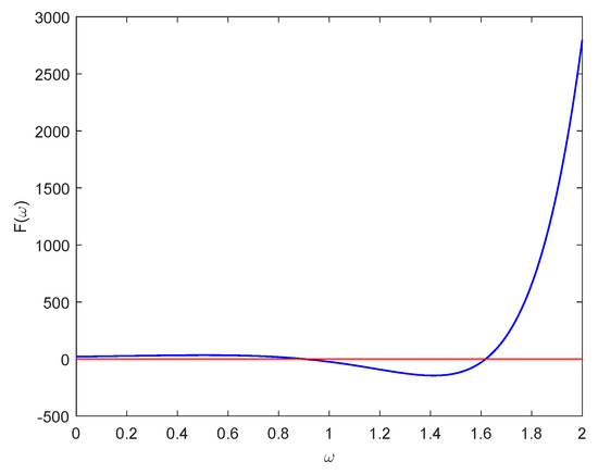
Figure 2. Graph of $F\left(\omega \right)$.

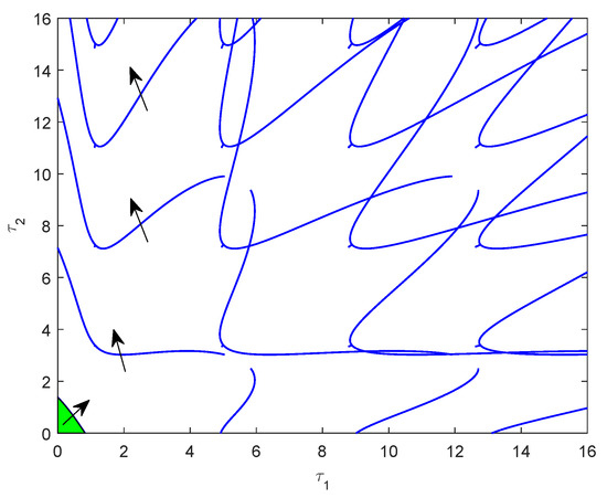
Figure 3. Stability switching curves.

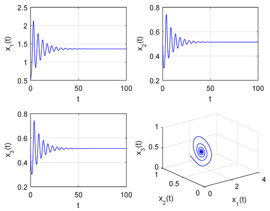
Figure 4. $E^{\ast }$ is locally asymptotically stable when ${\tau }_1=0.2,{\tau }_2=0.8$.

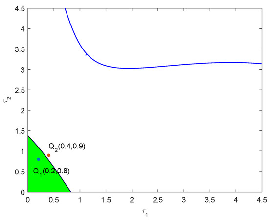
Figure 5. A partial enlargement of Figure 3.

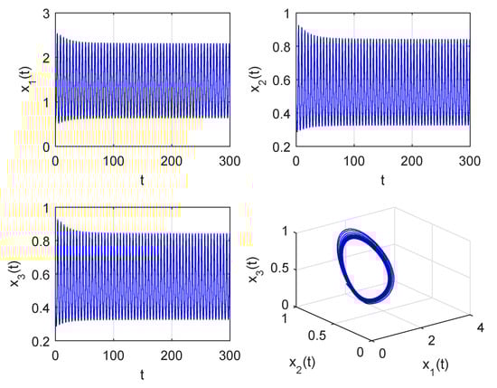
Figure 6. A periodic solution occurs at $E^{\ast }$ when ${\tau }_1=0.4,{\tau }_2=0.9$.

5. Conclusions

In this paper, a three-dimensional fractional predator–prey model with two nonidentical delays was proposed. We mainly studied the local stability switching and Hopf bifurcation induced by two delays. The stability switching curves were calculated. Furthermore, the stability switching of the system was found. The change in the direction of the stability of the system was determined by calculating the value of $\delta \left(\omega \right)$. The system keeps the steady state in the stable region. Choosing two delays as the bifurcation parameters, the conditions for the occurrence of the Hopf bifurcation of System (2) were derived. It was shown that the trajectory of the system is the axial symmetry (see Figure 6). Finally, a simulation example illustrated the validity of the theoretical analysis.

For System (2), the variation of gestation delay and hunting delay are the key factors in the stability of the system. When the value $({\tau }_1,{\tau }_2)$ is located in the stable region, the predator and prey can coexist. When the value $({\tau }_1,{\tau }_2)$ passes through the stability switching curves, the population of the three species demonstrates periodic oscillations. Moreover, when choosing the fractional order q = 0.84, 0.90, 0.94, 0.99, its corresponding crossing sets are given as ${\mathsf{\Omega }}_1=[0.9135,1.6392]$, ${\mathsf{\Omega }}_2=[0.9569,1.6202]$, ${\mathsf{\Omega }}_3=[0.9852,1.6102]$, ${\mathsf{\Omega }}_4=[1.0202,1.6002]$, respectively. The stability switching curves of System (30) are shown in Figure 7. Clearly, from Figure 7, we know that the stability region of the system shrinks when the fractional order increases. In order to observe Figure 7, we give a partial enlargement of Figure 7, as shown in Figure 8. However, we chose two delays as the bifurcation parameter in this paper. However, choosing the fractional order as the bifurcation parameter for the stability analysis of the fractional-order predator–prey model with two delays was not considered, which is the focus of our further research.

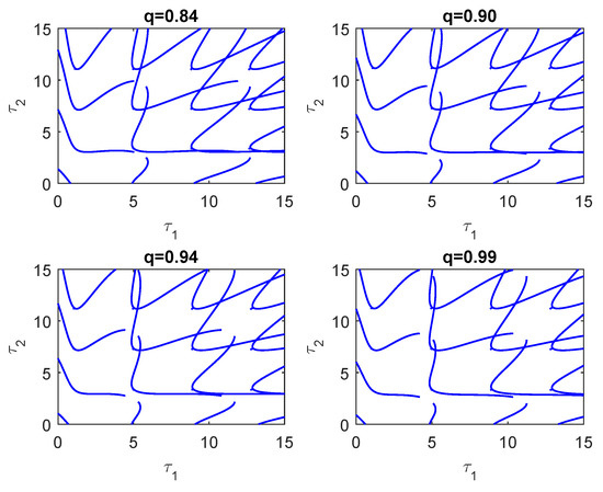
Figure 7. The stability switching curves of System (2) under different fractional orders.

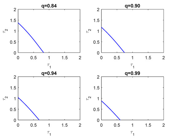
Figure 8. A partial enlargement of Figure 7.

References

- Javidi, M.; Nyamoradi, N. Dynamic analysis of a fractional order prey-predator interaction with harvesting. Appl. Math. Model. 2013, 37, 8946–8956. [Google Scholar] [CrossRef]
- Li, W.; Ji, J.; Huang, L.; Guo, Z. Global dynamics of a controlled discontinuous diffusive SIR epidemic system. Appl. Math. Lett. 2021, 121, 107420. [Google Scholar] [CrossRef]
- Li, W.; Ji, J.; Huang, L. Dynamics of a controlled discontinuous computer worm system. Proc. Am. Math. Soc. 2020, 148, 4389–4403. [Google Scholar] [CrossRef]
- Perumal, R.; Munigounder, S.; Mohd, M.H. Stability analysis of the fractional order prey-predator model with infection. Int. J. Simul. Model. 2020, 2020, 1–17. [Google Scholar]
- Dubey, B.; Kumar, A. Dynamics of prey-predator model with stage structure in prey including maturation and gestation delays. Nonlinear Dyn. 2019, 96, 2653–2679. [Google Scholar] [CrossRef]
- Hu, G.P.; Li, W.T.; Yan, X.P. Hopf bifurcations in a predator–prey system with multiple delays. Chaos Solitons Fractals. 2009, 42, 1273–1285. [Google Scholar] [CrossRef]
- Deng, W. Short memory principle and a predictor-corrector approach for fractional differential equations. J. Comput. Appl. Math. 2007, 206, 174–188. [Google Scholar] [CrossRef] [Green Version]
- Mandelbrot, B.B. The Fractal Geometry of Nature; WH Freeman: New York, NY, USA, 1982. [Google Scholar]
- Rihan, F.A. Numerical Modeling of fractional-order biological systems. Abstr. Appl. Anal. 2013, 2013, 816803. [Google Scholar] [CrossRef] [Green Version]
- Huang, C.; Liu, H.; Shi, X. Bifurcations in a fractional-order neural network with multiple leakage delays. Neural Netw. 2020, 131, 115–126. [Google Scholar] [CrossRef]
- You, X.; Song, Q.; Zhao, Z. Existence and finite-time stability of discrete fractional-order complex-valued neural networks with time delays. Neural Netw. 2020, 123, 248–260. [Google Scholar] [CrossRef]
- Diethelm, K. A fractional calculus based model for the simulation of an outbreak of dengue fever. Nonlinear Dyn. 2013, 71, 613–619. [Google Scholar] [CrossRef]
- Dhar, B.; Gupta, P.K.; Sajid, M. Solution of a dynamical memory effect COVID-19 infection system with leaky vaccination efficacy by non-singular kernel fractional derivatives. Math. Biosci. Eng. 2022, 19, 4341–4367. [Google Scholar] [CrossRef]
- N’Doye, I.; Voos, H. Chaos in a fractional-order cancer system. In Proceedings of the 2014 European Control Conference (ECC), Strasbourg, France, 24–27 June 2014; pp. 171–176. [Google Scholar]
- Zhao, H.; Lin, Y.; Dai, Y. Bifurcation analysis and control of chaos for a hybrid ratio-dependent three species food chain. Appl. Math. Comput. 2011, 218, 1533–1546. [Google Scholar] [CrossRef]
- Owolabi, K.M.; Atangana, A. Spatiotemporal dynamics of fractional predator–prey system with stage structure for the predator. Int. J. Appl. Comput. Math. 2017, 3, 903–924. [Google Scholar] [CrossRef]
- Tian, J.; Yu, Y.; Wang, H. Stability and bifurcation of two kinds of three-dimensional fractional Lotka–Volterra systems. Math. Probl. Eng. 2014, 2014, 695871. [Google Scholar] [CrossRef] [Green Version]
- Xie, Y.; Wang, Z.; Meng, B. Dynamical analysis for a fractional-order prey-predator model with Holling III type functional response and discontinuous harvest. Appl. Math. Lett. 2020, 106, 106342. [Google Scholar] [CrossRef]
- Huang, C.; Cao, J. Impact of leakage delay on bifurcation in high-order fractional BAM neural networks. Neural Netw. 2018, 98, 223–235. [Google Scholar] [CrossRef]
- Rihan, F.A.; Lakshmanan, S.; Hashish, A.H. Fractional-order delayed predator–prey systems with Holling type-II functional response. Nonlinear Dyn. 2015, 80, 777–789. [Google Scholar] [CrossRef]
- Huang, C.; Li, H.; Cao, J. A novel strategy of bifurcation control for a delayed fractional predator–prey model. Appl. Math. Comput. 2019, 347, 808–838. [Google Scholar] [CrossRef]
- Yuan, J.; Zhao, L.; Huang, C. Stability and bifurcation analysis of a fractional predator–prey model involving two nonidentical delays. Math. Comput. Simul. 2020, 181, 562–580. [Google Scholar] [CrossRef]
- Xu, C.; Aouiti, C.; Liu, Z. A further study on bifurcation for fractional order BAM neural networks with multiple delays. Neurocomputing 2020, 417, 501–515. [Google Scholar] [CrossRef]
- Xu, C.; Liu, Z. Fractional-order bidirectional associate memory (BAM) neural networks with multiple delays: The case of Hopf bifurcation. Math. Comput. Simul. 2021, 182, 471–494. [Google Scholar] [CrossRef]
- Xu, C.; Liao, M.; Li, P. Influence of multiple time delays on bifurcation of fractional-order neural networks. Appl. Math. Comput. 2019, 361, 565–582. [Google Scholar] [CrossRef]
- Zeeman, M.L.; van den Driessche, P. Three-Dimensional Competitive Lotka–Volterra Systems with no Periodic Orbits. Siam J. Appl. Math. 1998, 58, 227–234. [Google Scholar] [CrossRef]
- Gu, K.; Niculescu, S.I. On stability crossing curves for general systems with two delays. J. Math. Anal. Appl. 2005, 311, 231–253. [Google Scholar] [CrossRef] [Green Version]
- Lin, X.; Wang, H. Stability analysis of delay differential equations with two discrete delays. Can. Appl. Math. Q. 2012, 20, 519–533. [Google Scholar]
- Matsumoto, A.; Szidarovszky, F. Stability switching curves in a Lotka—Volterra competition system with two delays. Math. Comput. Simul. 2020, 178, 422–438. [Google Scholar] [CrossRef]
- Hale, J.K.; Huang, W.Z. Global geometry of the stable regions for two delay differential equations. J. Math. Anal. Appl. 1993, 178, 344–362. [Google Scholar] [CrossRef] [Green Version]
- An, Q.; Beretta, E.; Kuang, Y. Geometric stability switch criteria in delay differential equations with two delays and delay dependent parameters. J. Differ. Equ. 2019, 266, 7073–7100. [Google Scholar] [CrossRef]
- Li, H.; Huang, C.; Li, T. Dynamic complexity of a fractional-order predator–prey system with double delays. Physica A 2019, 526, 120852. [Google Scholar] [CrossRef]
- Zhao, L.; Huang, C.; Cao, J. Dynamics of fractional-order predator–prey model incorporating two delays. Fractals 2021, 29, 2150014. [Google Scholar] [CrossRef]
- Deng, W.; Li, C.; Lü, J. Stability analysis of linear fractional differential system with multiple time delays. Nonlinear Dyn. 2007, 48, 409–416. [Google Scholar] [CrossRef]
Publisher’s Note: MDPI stays neutral with regard to jurisdictional claims in published maps and institutional affiliations. |
© 2022 by the authors. Licensee MDPI, Basel, Switzerland. This article is an open access article distributed under the terms and conditions of the Creative Commons Attribution (CC BY) license (https://creativecommons.org/licenses/by/4.0/).