Article

A Novel Classification Framework for Hyperspectral Image Data by Improved Multilayer Perceptron Combined with Residual Network

Heilongjiang Province Key Laboratory of Laser Spectroscopy Technology and Application, Harbin University of Science and Technology, Harbin 150080, China
*
Author to whom correspondence should be addressed.
Symmetry 2022, 14(3), 611; https://doi.org/10.3390/sym14030611
Submission received: 22 February 2022 / Revised: 15 March 2022 / Accepted: 16 March 2022 / Published: 18 March 2022

Abstract

:
Convolutional neural networks (CNNs) have attracted extensive attention in the field of modern remote sensing image processing and show outstanding performance in hyperspectral image (HSI) classification. Nevertheless, some hyperspectral images have fixed position priors and parameter sharing between different positions, so the common convolution layer may ignore some important fine and useful information and cannot guarantee to effectively capture the optimal image features. This paper proposes an improved multilayer perceptron (IMLP) and IMLP combined with ResNet (IMLP-ResNet) two models for HSI classification. Combined with the characteristics of hyperspectral data, we design IMLP based on three improvements. Specifically, a depthwise over-parameterized convolutional layer is introduced to increase learnable parameters of the model in IMLP, which speeds up the convergence of the model without increasing the computational complexity. Secondly, a Focal Loss function is used to suppress the useless ones in the classification task and enhance the critical spectral–spatial features, which allow the IMLP network to learn more useful hyperspectral image information. Furthermore, to enhance the convergence speed of the network, cosine annealing is introduced to further improve the training performance of IMLP. Furthermore, the IMLP module is combined with a residual network (IMLP-ResNet) to construct a symmetric structure, which extracts more advanced semantic information from hyperspectral images. The proposed IMLP and IMLP-ResNet are tested on the two public HSI datasets (i.e., Indian Pines and Pavia University) and a real hyperspectral dataset (Xuzhou). Experimental results demonstrate the superiority of the proposed IMLP-ResNet method over several state-of-the-art methods with the highest OA, which outperforms CNN by 8.19%, 6.28%, 5.59% and outperforms ResNet by 3.52%, 3.54%, 2.67% on Indian Pines, Pavia University and Xuzhou datasets, respectively, and demonstrates that the well-designed MLPs can also obtain remarkable classification performance of HSI.

1. Introduction

Hyperspectral images (HSI) generally consist of tens to hundreds of continuous spectral bands [1], and can provide rich spatial and spectral information simultaneously, which offers great potential for the subsequent information extraction and practical applications in people’s lives [2]. Therefore, HSI is becoming a valuable tool for monitoring the Earth’s surface, and is used in a wide range of applications, such as environmental monitoring [3], precision agriculture [4], military investigation [5], and so on.
Hyperspectral image classification (HSIC) is one of the hot issues in hyperspectral research. Taking advantage of rich spectral information, numerous classification methods have been developed. Support vector machine (SVM) [6] has good robustness to high-dimensional hyperspectral data. K-nearest neighbor (KNN) [7] is one of the simplest classifiers for HSI classification. Random forest (RF) [8] is an ensemble learning method that operates by constructing multiple decision trees in the training process. In addition to these, decision trees [9], extreme learning machines [10], sparse representation-based classifiers [11] and many other methods have been further adopted to improve the performance of hyperspectral image classification. Nevertheless, it is difficult to accurately distinguish different land-cover categories using the spectral information [12]. Zhan et al. [13] used factor analysis to learn effective spectral and spatial features, and applied a Large-margin Distribution Machine (LDM) to hyperspectral remote sensing image classification. Meanwhile, morphological profile-based methods [14] have been proposed to effectively combine spatial and spectral information.
However, the conventional methods are based on handcrafted spectral–spatial features [15], which heavily depend on professional expertise and are quite empirical. Deep learning-based methods can automatically extract spectral features, spatial features, or spectral–spatial features of HSIs for classification application. Chen et al. [16] proposed a stacked autoencoder (SAE) to extract the joint spectral–spatial features for completing accurate HSI classification. Li et al. [17] used a single restricted Boltzmann machine (RBM) and a multilayer DBN to extract spectral–spatial features and obtained superior classification performance compared to the SVM-based method. Makantasis et al. [18] introduced a 2-D CNN to HSI classification, which achieved satisfactory performance with encoded spectral–spatial information with CNN and conducted classification with a multilayer perceptron. Chen et al. [19] used 3-D CNN to simultaneously extract spectral–spatial features and achieved a better result for HSI classification. Nonetheless, due to the loss of information caused by the vanishing gradient problem, training deep CNNs is still a little difficult. Recently, He et al. [20] proposed the residual network (ResNet) to solve this problem well, which defines a residual block as infrastructure elements to facilitate learning of deeper networks and enabling them to be substantially deeper. Zhong et al. [21] designed a spectral–spatial residual network (SSRN), which uses spectral residual blocks and spatial residual blocks consecutively to learn deep discriminative features from abundant spectral features and spatial contexts of HSI and achieved the most advanced HSI classification accuracy on agricultural, urban–rural and urban datasets. Moreover, a deep pyramidal residual network (PyResNet) [22] was developed to learn more robust spectral–spatial representations from the HSI cubes and provided competitive advantages (in terms of both classification accuracy and computational time) over the most advanced HSI classification methods.
Although CNN-based models have achieved good performance for HSI classification, the intrinsic complexity of remote sensing hyperspectral images still limits the performance of many models based on CNN. Firstly, the parameters of CNN increase exponentially with the convolution layer, and the size becomes lager with the increase in computing power. In addition, due to the long-running multiplication and addition time, the consumption of calculation has become the bottleneck of practical application. Finally, the translation invariance and local connectivity of CNN will affect the HSI classification effect. MLP, as a neural network with less constraints, can eliminate the negative effects of translation invariance and local connectivity and has been proven to be a promising machine learning technology. The present MLP-Mixer [23] is known as a pioneering MLP model. Furthermore, Liu et al. [24] proposed gMLP, which is based on MLPs combined with gating, and showed that it can perform as well as transformers in vision applications and key language. H. Touvron et al. [25] proposed ResMLP network structure built entirely upon multi-layer perceptron and attained surprisingly good accuracy/complexity tradeoffs on ImageNet. In addition, RaftMLP [26] aims to achieve cost-effectiveness and ease of application to downstream tasks with fewer resources in developing a global MLP-based model.
MLP solves translation invariance and local connectivity problems; residual networks can prevent model degradation and facilitate rapid convergence due to the retention of original information. Therefore, we proposed two MLP-based classification framework: an improved MLP (IMLP) model, and IMLP combined with ResNet (IMLP-ResNet) to achieve superior HSI classification performance in this paper.
As a summary, the following are the main contributions of this study.
  • MLP, as a less constrained network, can eliminate the negative effects of translation invariance and local connectivity. Therefore, this paper introduces MLP into HSI classification to fully obtain the spectral–spatial features of each sample and improve the classification performance of HSI.
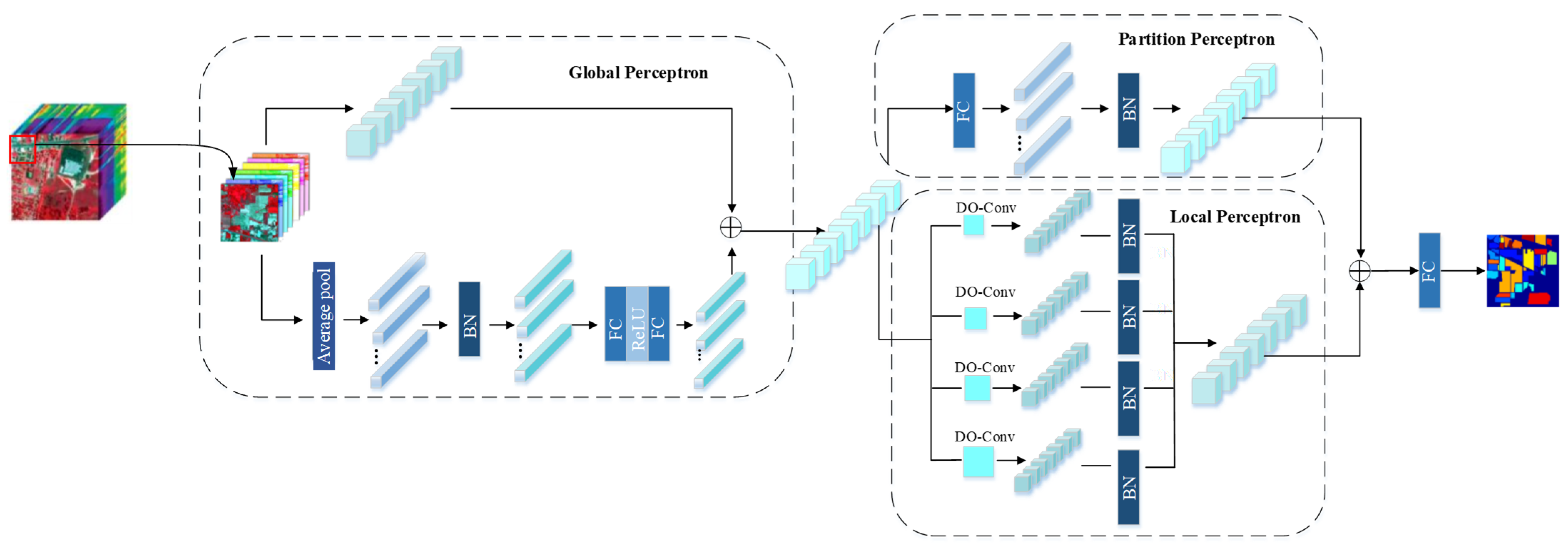
  • Based on the characteristics of hyperspectral images, we designed IMLP by introducing depthwise over-parameterized convolution, a Focal Loss function and a cosine annealing algorithm. Firstly, in order to improve network performance without increasing reasoning computation, depthwise over-parameterized convolutional layer replaced the ordinary convolution, which can speed up training with more parameters. Secondly, a Focal Loss function is used to enhance the important spectral–spatial features and prevent useless ones in the classification task, which allows the network to learn more useful hyperspectral image information. Finally, a cosine annealing algorithm is introduced to avoid oscillation and accelerate the convergence rate of the proposed model.
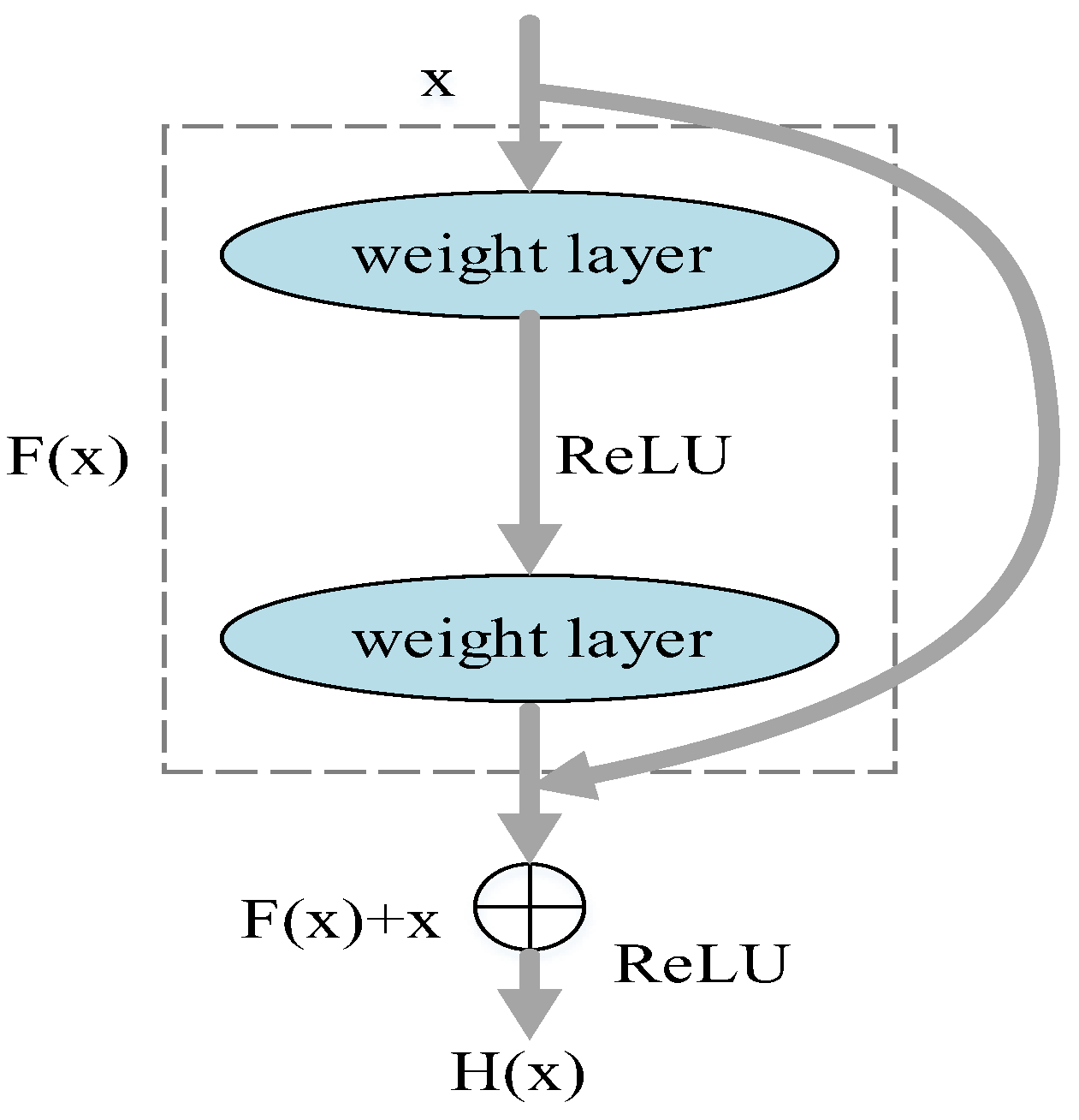
  • This paper inserts IMLP between two 3 × 3 convolutional layers in the ordinary residual block, called as IMLP-ResNet, which has a stronger ability to extract deeper features for HSI. Firstly, the residual structure can retain the original characteristics of the HSI data, and avoid the issues of gradient explosion and gradient disappearance during the training process. In addition, the residual structure can improve the modeling ability of the model. Moreover, IMLP can improve the feature extraction ability of residual network, so that the model strengthens the key features on the basis of retaining the original features of hyperspectral data.
The rest of this article is organized as follows. Section 2 describes our proposed classification approach. Section 3 reports the experimental results and appraises the performance of the proposed method part. Section 4 gives the discussion and analyzes how to choose experimental parameters in the IMLP-ResNet classification model. Section 5 gives the final conclusions and discusses research directions in the future.

2. The Proposed MLP-Based Methods for HSI Classification

Considering that the deepening of network layers in deep learning will cause the phenomenon of gradient disappearance and gradient explosion, the classification model adopts residual network as the basic framework. Figure 1 shows the overview flowchart of the improved MLP combined with ResNet (IMLP-ResNet) for HSI classification.
First of all, the improved MLP (IMLP) model for HSI classification is described in detail.

2.1. The Proposed Improved MLP (IMLP) for HSI Classification

Figure 2 gives the overall architecture of the proposed IMLP for HSI classification, which consists of two stages: a training stage and a testing stage. In the training stage, the network consists of a Global Perceptron module, Partition Perceptron module and Local Perceptron module. The structural reparameterization means that the training-time model has a set of parameters and the inference-time model has another set [27], and parameterizes the latter with the former’s parameters. The detailed description is explained as follows. It is assumed that the HSI dataset is the size of H × W × n B a n d , where H and W represent spatial height and width, and n B a n d is the frequency band number. First, each pixel of the hyperspectral image is processed with a fixed window size y × x , and a single sample with a shape of y × x × n B a n d is generated. Subsequently, with the shape of each patch, it becomes R × R × n B a n d . In this paper, the patch size is set to 4 × 4 .
The global perceptron module block consists of two branches. The first branch of the global perceptron module splits up the input hyperspectral feature image. The hyperspectral feature map changes from ( H , W , C ) to ( h 1 , w 1 , O ) In the second branch, the original feature map ( H , W , C ) is evenly pooled, and the size of the hyperspectral feature map becomes ( h , w ,   O ). H , W , C indicate the height, width and number of input channels of the input hyperspectral feature map, respectively. h 1 , w 1 , O respectively represent the height, width and number of output channels of the split hyperspectral feature image. Finally, h ,   w indicate the height and width of the hyperspectral feature image after average pooling as follows:
h 1 = H h   ,   w 1 = W w
The second branch uses average pooling to achieve a pixel for each hyperspectral feature image, and then feeds it though BN and a two-layer MLP. The hyperspectral feature map ( h , w , O ) is sent to the BN layer and two fully connected layers. The ReLU function is introduced between the two fully connected layers to effectively avoid gradient explosion and gradient disappearance. For the fully connected layer, X ( i n )   a n d   X ( o u t ) represent input and output, and the kernel W R Q × P is the matrix multiplication (MMUL) defined as follows:
X ( o u t ) = M M U L ( X ( i n ) , W ) = X ( i n ) W T
The hyperspectral vector is transformed into ( 1 , 1 , C ) by BN layer and two fully connected layers, after which the hyperspectral feature images are obtained after all branches are added. Then, the hyperspectral features are input to partition perceptron and local perceptron without dividing.
The Partition Perceptron module block contains a BN layer and a group convolution. The input of the partition perceptron is ( h , w , O ) . Then access the group convolution of groups = 4 and BN layer. After BN layer and a group convolution processing, it becomes the original hyperspectral feature input ( H , W , C ) .   Y ( o u t ) R C × H × W   indicates the output hyperspectral feature. p   is the number of pixels filled, while F R C / g × K × K is the convolution kernel. g indicates the number of convolution groups. The calculation formula of Y ( o u t ) is shown in Equation (3).
Y ( o u t ) = g ( Y ( i n ) , F , g , p ) ,   F R C / g × K × K
The Local Perceptron module contains a depthwise over-parameterized convolutional layer (DO-Conv) [28] and a BN layer. First, the local perceptron module sends the segmented hyperspectral feature image ( h , w , O ) simultaneously to the deep hyperparametric convolution layer. Then the feature graph is fed into BN layer, and the output of all convolution branches is added with the output of the partition perceptron as the final output. In the test phase, reparameterization is carried out to fuse the two parts of the local perceptron module and the partitioned perceptron module into a fully connected layer. The FC kernel of a DO-Conv kernel is the result of convolution on an identity matrix with proper reshaping operation. Formula (4) shows exactly how to build   W ( F , p ) from F   a n d   p .
W ( F , p ) = D O C O N V ( Y , F , p ) , ( C h w , O h w ) T
In order to increase the learnable parameters of the proposed model, a deeply over-parameterized convolutional layer is introduced to replace the ordinary convolutional layer to construct IMLP. In addition, IMLP introduced Focal Loss for the purpose of solving the problem of data imbalance in hyperspectral image classification and the cosine annealing algorithm to improve the training performance of IMLP, which makes the convergence speed of the network faster. The three modifications are described in the following parts.

2.1.1. DO-Conv

In order to improve the training speed of the model, DO-Conv is introduced to replace the traditional convolution layer in the local perceptron module. The architecture of DO-Conv is shown as Figure 3. There are two components in DO-Conv, including a feature component and a convolution kernel component. The model is more efficient after adding the convolution kernel component, so this paper uses the convolution kernel component to train the network. The DO-Conv is composed of a conventional convolution W R C o u t × D m u l × C i n and a deep convolution.   D R ( M × N ) × D m u l × C i n . In conventional convolution, the convolution layer slides the input data, and each element of the output feature is obtained by the horizontal slice of the convolution kernel and P dot product of the image block. In the deep convolution layer, the convolution kernel is convolved with each input channel during the training phase.
At the end of the training phase, the multi-layer composite linear operation used for over-parameterization is folded into a compact single-layer representation. Then, only one layer is used for reasoning, reducing the calculation to full equivalence with the regular layer. M and N are spatial dimensions of , C i n is the number of input feature graphs, C o u t is the number of D m u l output feature graphs,   D T R D m u l × ( M × N ) × C i n is the transposition of D R D m u l × ( M × N ) × C i n and the convolution kernel of DO-Conv is W . First, the deep convolution kernel D T and the convolution kernel of ordinary convolution W are combined into W , W = D T W . The convolution output feature O is then generated as O = W , where is convolution, is the dot product, and # is the defined operator.
O = ( D , W ) # P = ( D ^ T W ) P

2.1.2. Focal Loss

Data imbalance is common in hyperspectral remote sensing images. Because there are various objects with different sizes in a hyperspectral scene, it is very difficult to mark samples in practice. Therefore, there is usually a serious imbalance between various samples of hyperspectral data [29]. Thus, this paper introduced focal loss function instead of cross entropy loss (CE) function. CE is written as follows:
C E ( p , y ) = { log ( p )   i f   y = 1 log ( 1 p )   o t h e r w i s e
where y { ± 1 } specifies the ground-truth class and P [ 0 , 1 ] is the model’s estimated probability for the class with label y = 1 , and p t is defined as follows:
p t = { p   i f y = 1 1 p   o t h e r w i s e
Focal Loss is calculated as follows:
F L ( p t ) = ( 1 p t ) γ l o g ( p t )
Focusing parameter γ can adjust the weight of positive and negative samples as well as control the weight of difficult and easy samples. When some samples are misclassified and p t is very small, the regulatory factor ( 1 p t ) γ is close to 1, which has little influence on loss function. However, as p t tends to 1, this factor will gradually tend to 0, and losses for well-classified samples will also decrease, so as to achieve the effect of reducing weight. γ will smoothly adjust the proportion of reduced weights for easily classified samples. Increased γ can enhance the influence of the regulatory factor, which reduces the loss contribution of easily classified samples and broadens the range of low loss received by samples.

2.1.3. Cosine Annealing Algorithm

The batch gradient descent (BGD) and stochastic gradient descent (SGD) are mainly used to update parameter values in deep learning. BGD needs to update each parameter with all the data sets. If the sample size is too large, the training speed will be too slow, which will increase the computational cost. However, SGD has a characteristic fast training speed, because it uses part of the information of the data and easily falls into a local optimal solution [30]. Therefore, this article introduces the cosine annealing algorithm to update the parameter values under the premise of comprehensive training sample speed and computational cost, and the learning rate can be reduced by the cosine function. We decay the learning rate with a cosine annealing for each batch as follows:
η t = η m i n i + 1 / 2 ( η m a x i η m i n i ) ( 1 + c o s ( T c T i π ) )
where η m i n i and η m a x i are ranges for the learning rate, T i is the total number of epochs, and T c   is the current epoch. When T c = T i , η t reaches the minimum training batch.
When the gradient descent algorithm is used to optimize the objective function, the learning rate should become smaller to get closer to the global minimum value of the loss function and make the model as close as possible to this point. The cosine annealing algorithm can reduce the learning rate by cosine function. The cosine goes down slowly as x increases, then it accelerates and goes down slowly again.

2.2. The Proposed IMLP-ResNet Model for HSI Classification

The main idea of an IMLP-ResNet model refers to the insertion of IMLP between two 3 × 3 convolutional layers in the ordinary residual block; that is to say, the IMLP module inserted into the third layer of ResNet has a stronger ability to extract deeper features for HSI. First of all, ResNet34 can retain the original characteristics of the HSI data. It can solve gradient explosion and gradient disappearance in the training process. In the meantime, ResNet34 can improve the modeling ability of the model. IMLP can improve the feature extraction ability of residual network and strengthen the key features on the basis of retaining the original features. ResNet34 compared with other CNN models can help overcome the over-fitting phenomenon. The ResNet family includes ResNet18, ResNet34, ResNet50, ResNet152, etc. In order to improve the classification efficiency, ResNet34 with fewer parameters was used in this paper.

2.2.1. The Structure of ResNet34

The classification performance of the deep learning model decreases with the increase in depth [31]. Inspired by deep residual learning framework, this aggravating problem can be solved by adding quick connections and propagating eigenvalues between each layer.
The core of the deep residual network lies in the residual learning module, which can save part of the original input information during the training of the deep CNN model [32,33]. In this way, the learning target is transferred to avoid the saturation of classification accuracy caused by the depth of the network. As shown in Figure 4, x represents the input, H ( x ) represents the output, and F ( x ) represents the residual function. The output of the residual unit is shown in Equation (10).
H ( x ) = F ( x ) + x
The residual module calculates the residual error when the span is not interrupted. { W i } is used to show the residual module block, the residual module actually calculates the output result as shown in Equation (11).
y = F ( x , { W i } ) + x
F ( x , { W i } ) is residual mapping and can be obtained by back propagation (BP). For the case of two weight layers, the calculation process is shown in Equation (12) when the bias is ignored.
F ( x , { W i } ) = W 2 σ ( W 1 ) x = W 2 R e L U ( W 1 ) x
The calculation of residual module requires that F ( x , { W i } ) and x have the same dimension. A linear projection W s is proposed by the shortcut connections to match the dimensions:
y = F ( x , { W i } ) + W s x
Figure 5 is the overall architecture of ResNet34, which adds shortcut connections between each two layers, and can directly sample the input image with the convolution of stride of 2. It can be seen that there are four layers in the structure of ResNet34 and each layer has 3, 4, 6, and 3 residual blocks, respectively. The convolutional layers mostly have 3 × 3 filters for the same output feature map size. In order to maintain the time complexity of each layer, the number of filters was doubled if the feature map size is halved. The size of the feature map is halved and the number of feature maps is doubled to maintain the complexity of the network.

2.2.2. IMLP-ResNet Model

Figure 6a shows the structure of the ordinary residual block, which contains two 3 × 3 convolutional layers and a shortcut connection. BN is applied after the convolutional layer and before the activation function to accelerate the convergence of the module. The shortcut connection enables the gradient to propagate directly from the later to earlier layers, thus mitigating the gradient vanishing. The stacking multiple residual blocks can develop a deeper network to alleviate overfitting of the network.
As shown in Figure 6b, this paper inserts IMLP between two 3 × 3 convolutional layers in the ordinary residual block to constitute a symmetric structure. Traditional convolutional layers obtain long-range dependencies by the large receptive fields formed by deep stacks of convolutional layers. However, repetition of local operations requires a lot of computation and may cause optimization difficulties. At the same time, some images have intrinsic positional prior, which cannot be fully utilized by a convolutional layer because it shares parameters among different positions. IMLP runs faster than CNN with the same number of parameters and has global capacity and positional perception. Therefore, our proposed IMLP-ResNet can perform fine-feature extraction at different network levels and learn more comprehensive feature representations for HSI classification.

3. Results

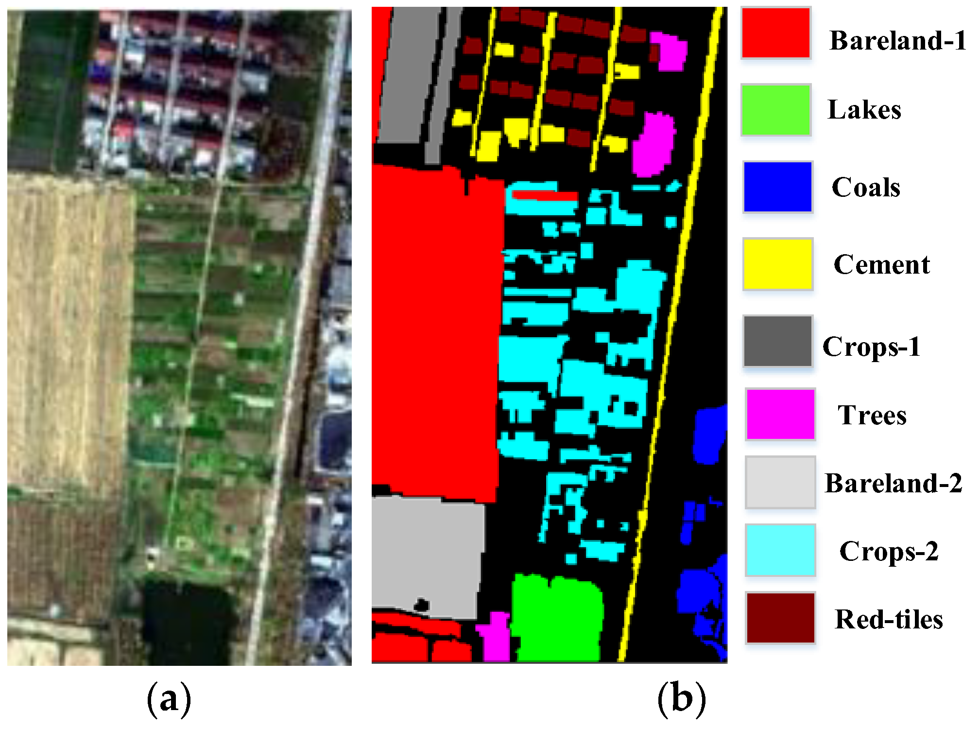
3.1. Dataset Description

In order to verify the classification performance efficiently, a number of experiments were performed on two standard hyperspectral datasets (Indian Pines and Pavia University), and the Xuzhou dataset. The Indian Pines dataset was acquired in 1992 by an Airborne Visible-Infrared Imaging Spectrometer (AVIRIS) sensor at the Indian Pines Test Site in northwestern Indiana with a size of 145 × 145 pixels, 224 spectral bands and 16 types of land cover. The number of bands was reduced to 200 by removing the bands covering the water-absorbing area (bands 104–108, 150–163, 220). The Pavia University dataset was picked up by ROSIS sensors flying over Pavia in northern Italy. The number of spectral bands is 103, and the size is 610 × 610 pixels with nine categories. Figure 7 and Figure 8 show the false-color composite image and ground truth map, and Table 1 and Table 2 report the detailed number of pixels available in each class for the two datasets respectively.
The Xuzhou dataset was obtained via a HySpex SWIR-384 and HySpex VNIR-1600 imaging spectroradiometer in Xuzhou in November 2014, with a size of 500 × 260 pixels and 436 bands. Based on the field survey, nine feature types were identified. Figure 9 shows the false-color composite image and the ground truth graph. Table 3 reports the detailed number of pixels available in each class.

3.2. Experimental Parameters Setting

All experiments were performed on an Intel(R) Xeon(R) 4208 CPU @ 2.10 GHz processor and Nvidia GeForce RTX 2080Ti graphics card. In order to reduce experimental errors, the model randomly selected a limited number of samples from the training set for training. The epoch was set to 200, and the batch size was set to 32. All experimental results were averaged from 10 experiments. Overall accuracy (OA), average accuracy (AA) and Kappa coefficient (K) were used as evaluation indexes to measure the performance of each method. This model uses Adam optimizer to learn the weight of three-dimensional spectral space filter, and adopts cosine annealing to adjust the learning rate, taking cosine function as the period, and resetting the learning rate at the maximum value of each period. The initial learning rate of this method was 0.001, with a cycle of 15 epochs. After 15 epochs, the learning rate was automatically increased and the local optimum was skipped.

3.3. Evaluation Metrics

The evaluation index is the standard to evaluate the quality of the algorithm model, which guides us to better improve the algorithm’s classification performance. In this experiment, the Confusion Matrix is used to count the classification results, and the Overall Accuracy (OA), Average Accuracy (AA) and Kappa coefficient (K) are used to evaluate the classification results.
Confusion Matrix is a kind of evaluation matrix commonly used in classification problems. Each row of the matrix represents the number vector of a category divided into all classes, and each column represents the number vector of all categories divided into all classes. As shown in Formula (14), the diagonal elements of the matrix are the number of correctly classified categories of a certain category, where C is the number of categories of classification problems, and m i j represents the ith class samples misclassified into the j th class.
M = [ m 11 m 12 m 21 m 22 m 1 j m 2 j m 1 C m 2 C m i 1 m i 2 m i j m i C m C 1 m C 2 m C j m C C ]
OA computes to the ratio between the number of correctly classified samples and that of the total samples to be tested. This index is a common evaluation standard for classification problems and reflects the probability of consistency between classification results and real reference values, as written in Formula (15).
O A = t r a c e ( M ) N
where t r a c e ( M ) is the trace of the matrix, that is, the sum of all elements on the main diagonal of matrix M, and N is the total number of all test samples.
AA represents the average classification accuracy of each category, which reflects the average performance of all categories. m i + represents the sum of all elements in row i, and C represents the total number of categories.
A A = Σ i = 1 N m i i m i + C
K is an index to measure the classification accuracy, which can evaluate the classification performance more comprehensively by integrating the overall classification accuracy and average classification accuracy.
K = N Σ i = 1 C m i i Σ i = 1 C m i + m + i N 2 Σ i = 1 C m i + m + i
where m i + represents the   i th row of the confusion matrix, and m + i represents the i th column of the Confusion Matrix.

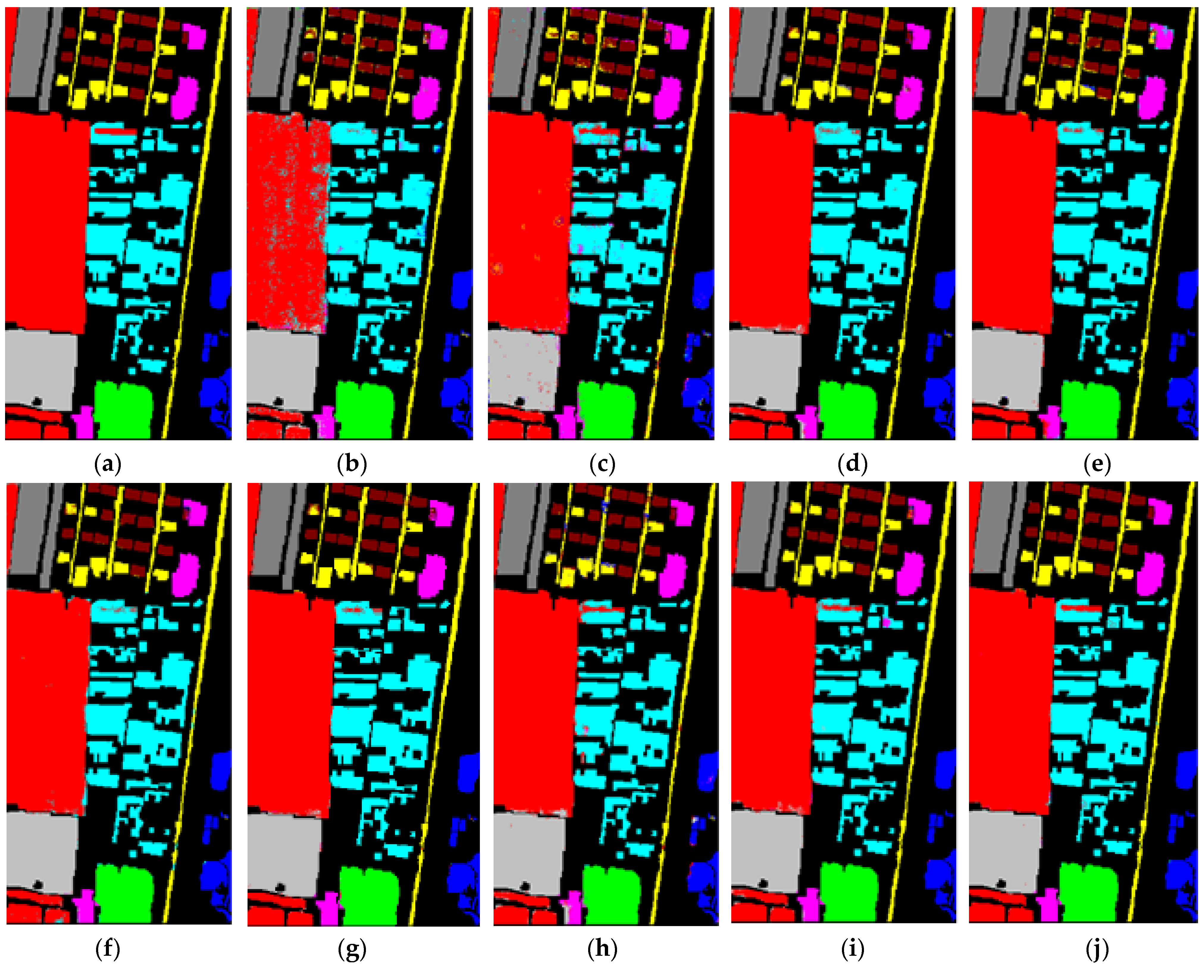
3.4. Comparison of the Proposed Methods with the State-of-the-Art Methods

The curves of the loss and accuracy of the training and testing of all datasets classified by the proposed IMLP-ResNet over 200 epochs are shown in Figure 10, Figure 11 and Figure 12. It can be observed from Figure 10a, Figure 11a and Figure 12a that, with the increase in the number of epochs in the Indian Pines, Pavia University and Xuzhou datasets, the losses in training sets and validation sets decreased continuously. In Figure 10b, Figure 11b and Figure 12b, classification accuracy keeps improving. The Indian Pines dataset and Pavia University dataset converged around epoch 180, while the Xuzhou dataset converged around the epoch of 190. Among them, the Xuzhou data set converges slowly compared with the other two data sets, because the number of training samples in this dataset is higher than the other two datasets. However, the accuracy of the training set and validation set of the three datasets is still improved after the model converges. The main reason is that, with the continuous optimization of parameters, the gradual fitting of curves verifies the good generalization ability of our proposed model and the convergence of this model.
The experiment mainly compared the proposed algorithm with the Radial Basis Function (RBF) Support Vector Machine algorithm (RBF-SVM) [34] and Extended Morphological Profile (EMP) Support Vector Machine Calculation Methods (EMP-SVM) [35], Deep Convolutional Neural Network (DCNN) [36], Spectral–Spatial Residual Network (SSRN) [21], Residual Network (ResNet) [37], Pyramid Residual network (PyResNet) [22], RepMLP [38], IMLP classification performance for hyperspectral dataset. Ten percent of the total sample number was used as the training sample number for hyperspectral classification as shown in Table 4, Table 5 and Table 6. Compared with other methods, the IMLP-ResNet proposed in this paper has the highest classification accuracy for the three datasets. For example, compared with RBF-SVM in the Indian Pines dataset, IMLP-ResNet increased OA, AA and K by 12.85%, 12.87% and 10.55% and improved by 0.54%, 0.70% and 0.58% compared with RepMLP, respectively. Taking the Xuzhou dataset as an example, OA reached 98.15%, compared with RBF-SVM, EMP-SVM, DCNN, SSRN, ResNet, PyResNet, RepMLP and IMLP, in which OA increased by 15.89%, 10.72%, 5.59%, 3.98%, 2.67%, 1.80%, 1.37% and 1.01% respectively. The Indian Pines dataset and Pavia University dataset have similar classification results. All the experimental results show that the proposed IMLP-ResNet is superior to other methods.
Figure 13, Figure 14 and Figure 15 show the classification diagram of different methods for all datasets of 10% training samples. Compared with the classical EMP-SVM method and deep learning-based DCNN, SSRN, ResNet and other methods, the proposed classification model in this paper has more accurate classification results. Taking Pavia University dataset as an example, the traditional RBF-SVM and EMP-SVM methods have many noise points in classification results.
As shown in Figure 14, parts of the traffic land are mistakenly classified as grassland, and the classification accuracy of ground objects is relatively low. Compared with SVM, DCNN and SSRN classification methods, the classification effect of ResNet and PyResNet is improved, but there are still some misclassification phenomena. However, the IMLP-ResNet model can make full use of each convolutional layer and feature map, and the classification effect is greatly improved. It also eliminates block misclassification and protects edge information. Experiments show that IMLP–ResNet can effectively extract more refined features from three kinds of data sets and cross-dimensional information interaction focuses on more important features, thus improving the classification accuracy.
Figure 15 shows the classification results of the Xuzhou dataset. Xuzhou is an important coal-producing area in China, and coal mining areas may lead to surface subsidence and soil quality degradation, which threatens the safety of residential areas and crop planting. At the same time, it may induce secondary geological disasters. Figure 15 can reflect the land-use situation of the mining area. According to the current classification results, there is still a large area of cultivated land around the tailings pond. By classifying all kinds of ground objects in the test area, we can understand the distribution of the tailings pond, which is helpful to the later mining area.

4. Discussions

In order to find the optimal architecture, it is necessary to do experiments with different main parameters, which plays a crucial role in the size of the model and the complexity of the proposed IMLP–ResNet. By comparing the overall accuracy of different parameters, the influence of these parameters on the model can be analyzed. In the Indian Pines dataset, Pavia University dataset and Xuzhou dataset, the improvement effects of different parameter changes on the model are shown in Figure 16, Figure 17, Figure 18 and Figure 19.
The first parameter was experimentally verified in a different patch size. The hyperspectral images were first divided into fixed-size patches to input IMLP-ResNet, and patch sizes were set as 4 × 4 ,   8 × 8 ,   16 × 16 respectively. The corresponding input dataset is divided into 4 × 4 × n B a n d ,   8 × 8 × n B a n d , and 16 × 16 × n B a n d . As shown in Figure 16, for the three datasets, OA, AA and Kappa coefficients all showed a decreasing trend with the increase in patch size. When patch size = 4, the IMLP-ResNet model proposed achieves the best classification accuracy, because the correlation between the internal information of image patches weakens with the increase in patch size.
The second parameter is to choose the layer of ResNet into which the proposed IMLP module should be inserted to get the best classification results. As shown in Figure 17, we can conclude that the IMLP module inserted into the third layer of ResNet has the highest accuracy in the three datasets. This is because the number of residual blocks in ResNet34 is [3,4,6], that is, the number of residual blocks in the third layer is more than that in the other three layers. The IMLP module inserted in the third layer of ResNet has a deeper network than the other three layers, which has a stronger ability to extract deeper features of hyperspectral images, so the classification accuracy is higher.
The third parameter is the proportion of training samples to the total samples. The patch size is set to 4 and IMLP module is the third layer of ResNet; 5% and 10% of training samples are taken from the three data sets, respectively, as shown in Figure 18 and Figure 19.
It can be seen from Figure 18 and Figure 19 that, when the number of training samples accounts for 10% of the total samples, the OA is higher than when the number of training samples accounts for 5% of the total samples. This is because the more training samples exist, the more accurately the model can estimate the data distribution, thus the better the generalization performance in the validation set, which leads to higher accuracy. The above results show that when the patch size is 4, the IMLP module is inserted into the third layer of ResNet, and the number of training samples accounts for 10% of the total number of samples, the three datasets can achieve the best classification performance with our proposed IMLP-ResNet.

5. Conclusions

In this paper, two HSI classification frameworks based on MLP are proposed: the IMLP model and IMLP–ResNet. Firstly, according to the characteristics of HSI, three improvements were made to the original model and the IMLP was designed. Secondly, in order to improve the network performance without increasing the amount of inference computation, we introduced a deep over-parameterized convolution layer instead of ordinary convolution. Thirdly, in order to enable the network to learn more useful hyperspectral image information and suppress useless features, we used a Focal Loss function to enhance the key spectral spatial features in the classification task. Finally, in order to avoid oscillation, a cosine annealing algorithm is introduced to accelerate the convergence of the model. The residual structure can retain the original characteristics of this data, avoid the problems of gradient explosion and gradient disappearance in the training process, and improve the modeling ability of the model. In addition, IMLP can improve the feature extraction capability of ResNet, so that the model can enhance the key features while preserving the original features of hyperspectral data. Therefore, in this paper, we proposed IMLP–ResNet, which can extract 3D spectral–spatial features at different levels of the network and learn more comprehensive feature representation for HSI classification.
The proposed IMLP and IMLP–ResNet were tested on two public datasets (Indian Pine and Pavia) and a real HSI dataset (Xuzhou). Compared with the classic methods and deep learning-based methods, the proposed IMLP and IMLP-ResNet show obvious improvements. The results show that the proposed IMLP algorithm and IMLP–ResNet algorithm are meaningful and can obtain better classification results in HSI classification.
However, in the task of hyperspectral image classification, the available marker samples are usually very limited. When analyzing the classification effect of the number of training samples, the IMLP–ResNet proposed in this paper finds that the effect of 10% of the number of samples is better than 5%. Therefore, in the next step, we will consider data expansion, active learning, transfer learning, meta learning and other technologies to realize the construction and design of a network model combined with MLP under small samples. In addition, the means of using unlabeled samples more effectively for semi-supervised hyperspectral classification based on MLP is also worthy of further research.

Author Contributions

Conceptualization, A.W. and H.W.; methodology, software, validation, M.L.; writing—review and editing, H.W. and A.W. All authors have read and agreed to the published version of the manuscript.

Funding

This work was funded by the National Natural Science Foundation of China under Grant NSFC-61671190.

Data Availability Statement

The data are available at http://www.ehu.eus/ccwintco/index.php?%20title=Hyperspectral-Remote-Sensing-Scenes (accessed on 21 February 2022).

Acknowledgments

We thank Kaiyuan Jiang for his valuable comments and discussion.

Conflicts of Interest

The authors declare no conflict of interest.

References

  1. Hong, D.; Wu, X.; Ghamisi, P.; Chanussot, J.; Yokoya, N.; Zhu, X.X. Invariant attribute profiles: A spatial-frequency joint feature extractor for hyperspectral image classification. IEEE Trans. Geosci. Remote Sens. 2020, 58, 3791–3808. [Google Scholar] [CrossRef] [Green Version]
  2. Li, S.; Song, W.; Fang, L.; Chen, Y.; Ghamisi, P.; Benediktsson, J.A. Deep Learning for Hyperspectral Image Classification: An Overview. IEEE Trans. Geosci. Remote Sens. 2019, 57, 6690–6709. [Google Scholar] [CrossRef] [Green Version]
  3. Bioucas-Dias, J.M.; Plaza, A.; Camps-Valls, G.; Scheunders, P.; Nasrabadi, N.; Chanussot, J. Hyperspectral remote sensing data analysis and future challenges. IEEE Geosci. Remote Sens. Mag. 2013, 1, 6–36. [Google Scholar] [CrossRef] [Green Version]
  4. Zhang, X.; Sun, Y.; Shang, K.; Zhang, L.; Wang, S. Crop classification based on feature band set construction and object-oriented approach using hyperspectral images. IEEE J. Sel. Top. Appl. Earth Obs. Remote Sens. 2016, 9, 4117–4128. [Google Scholar] [CrossRef]
  5. Shimoni, M.; Haelterman, R.; Perneel, C. Hypersectral imaging for military and security applications: Combining myriad processing and sensing techniques. IEEE Geosci. Remote Sens. Mag. 2019, 7, 101–117. [Google Scholar] [CrossRef]
  6. Melgani, F.; Bruzzone, L. Classification of hyperspectral remote sensing images with support vector machines. IEEE Trans. Geosci. Remote Sens. 2004, 42, 1778–1790. [Google Scholar]
  7. Ma, L.; Crawford, M.M.; Tian, J. Local manifold learning-based-nearest-neighbor for hyperspectral image classification. IEEE Trans. Geosci. Remote Sens. 2010, 48, 4099–4109. [Google Scholar] [CrossRef]
  8. Ham, J.; Chen, Y.; Crawford, M.M.; Ghosh, J. Investigation of the random forest framework for classification of hyperspectral data. IEEE Trans. Geosci. Remote Sens. 2005, 43, 492–501. [Google Scholar] [CrossRef] [Green Version]
  9. Delalieux, S.; Somers, B.; Haest, B.; Spanhove, T.; Borre, J.V.; Mücher, C.A. Heathland conservation status mapping through integration of hyperspectral mixture analysis and decision tree classifiers. Remote Sens. Environ. 2012, 126, 222–231. [Google Scholar] [CrossRef]
  10. Li, W.; Chen, C.; Su, H.; Du, Q. Local binary patterns and extreme learning machine for hyperspectral imagery classification. IEEE Trans. Geosci. Remote Sens. 2015, 53, 3681–3693. [Google Scholar] [CrossRef]
  11. Chen, Y.; Nasrabadi, N.M.; Tran, T.D. Hyperspectral image classification using dictionary-based sparse representation. IEEE Trans. Geosci. Remote Sens. 2011, 49, 3973–3985. [Google Scholar] [CrossRef]
  12. He, L.; Li, J.; Liu, C.; Li, S. Recent advances on spectral–spatial hyperspectral image classification: An overview and new guidelines. IEEE Trans. Geosci. Remote Sens. 2017, 56, 1579–1597. [Google Scholar] [CrossRef]
  13. Zhan, K.; Wang, H.; Huang, H.; Xie, Y. Large margin distribution machine for hyperspectral image classification. J. Electron. Imaging 2016, 25, 63024. [Google Scholar] [CrossRef]
  14. Song, B.; Li, J.; Dalla Mura, M.; Li, P.; Plaza, A.; Bioucas-Dias, J.E.M.; Benediktsson, J.A.; Chanussot, J. Remotely sensed image classification using sparse representations of morphological attribute profiles. IEEE Trans. Geosci. Remote Sens. 2013, 52, 5122–5136. [Google Scholar] [CrossRef] [Green Version]
  15. Xue, F.; Tan, F.; Ye, Z.; Chen, J.; Wei, Y. Spectral-spatial classification of hyperspectral image using improved functional principal component analysis. IEEE Trans. Geosci. Remote Sens. 2021, 19, 1–5. [Google Scholar] [CrossRef]
  16. Chen, Y.; Lin, Z.; Zhao, X.; Wang, G.; Gu, Y. Deep learning-based classification of hyperspectral data. IEEE J. Sel. Top. Appl. Earth Obs. Remote Sens. 2014, 7, 2094–2107. [Google Scholar] [CrossRef]
  17. Li, T.; Zhang, J.; Zhang, Y. Classification of hyperspectral image based on deep belief networks. In Proceedings of the 2014 IEEE International Conference on Image Processing, Paris, France, 27 October 2014. [Google Scholar]
  18. Makantasis, K.; Karantzalos, K.; Doulamis, A.; Doulamis, N. Deep supervised learning for hyperspectral data classification through convolutional neural networks. In Proceedings of the 2015 IEEE International Geoscience and Remote Sensing Symposium, Milan, Italy, 26–31 July 2015; pp. 4959–4962. [Google Scholar]
  19. Chen, Y.; Jiang, H.; Li, C.; Jia, X.; Ghamisi, P. Deep feature extraction and classification of hyperspectral images based on convolutional neural networks. IEEE Trans. Geosci. Remote Sens. 2016, 54, 6232–6251. [Google Scholar] [CrossRef] [Green Version]
  20. He, K.; Zhang, X.; Ren, S.; Sun, J. Deep residual learning for image recognition. arXiv 2016, arXiv:1512.03385. [Google Scholar]
  21. Zhong, Z.; Li, J.; Luo, Z.; Chapman, M. Spectral–spatial residual network for hyperspectral image classification: A 3-d deep learning framework. IEEE Trans. Geosci. Remote Sens. 2017, 56, 847–858. [Google Scholar] [CrossRef]
  22. Paoletti, M.E.; Haut, J.M.; Fern; Ez-Beltran, R.; Plaza, J.; Plaza, A.J.; Pla, F. Deep pyramidal residual networks for spectral–spatial hyperspectral image classification. IEEE Trans. Geosci. Remote Sens. 2018, 57, 740–754. [Google Scholar] [CrossRef]
  23. Tolstikhin, I.; Houlsby, N.; Kolesnikov, A.; Beyer, L.; Zhai, X.; Unterthiner, T.; Yung, J.; Steiner, A.; Keysers, D.; Uszkoreit, J.; et al. Mlp-mixer: An all-mlp architecture for vision. arXiv 2021, arXiv:2105.01601. [Google Scholar]
  24. Liu, H.; Dai, Z.; So, D.; Le, Q. Pay attention to MLPs. Adv. Neural Inf. Processing Syst. arXiv 2021, arXiv:2105.08050. [Google Scholar]
  25. Touvron, H.; Bojanowski, P.; Caron, M.; Cord, M.; El-Nouby, A.; Grave, E.; Jégou, H. Resmlp: Feedforward networks for image classification with data-efficient training. arXiv 2021, arXiv:2105.03404. [Google Scholar]
  26. Tatsunami, Y.; Taki, M. Raftmlp: How much can be done without attention and with less spatial locality? arXiv 2021, arXiv:2108.04384. [Google Scholar]
  27. Zhang, M.; Zuo, X.; Chen, Y.; Liu, Y.; Li, M. Pose estimation for ground robots: On manifold representation, integration, reparameterization, and optimization. IEEE Trans. Robot. 2021, 37, 1081–1099. [Google Scholar] [CrossRef]
  28. Cao, J.; Li, Y.; Sun, M.; Chen, Y.; Lischinski, D.; Cohen-Or, D.; Chen, B.; Tu, C. DO-Conv: Depthwise over-parameterized convolutional layer. arXiv 2020, arXiv:2006.12030. [Google Scholar]
  29. Lin, T.Y.; Goyal, P.; Girshick, R.; He, K.; Dollar, P. Focal Loss for Dense Object Detection. IEEE Trans. Pattern Anal. Mach. Intell. 2020, 42, 318–327. [Google Scholar] [CrossRef] [Green Version]
  30. Loshchilov, I.; Hutter, F. Sgdr: Stochastic gradient descent with warm restarts. arXiv 2016, arXiv:1608.03983. [Google Scholar]
  31. Yuan, Y.; Wang, C.; Jiang, Z. Proxy-based deep learning framework for spectral-spatial hyperspectral image classification: Efficient and robust. IEEE Trans. Geosci. Remote Sens. 2021, 60, 1–15. [Google Scholar] [CrossRef]
  32. Chen, W.; Zheng, X.; Lu, X. Hyperspectral image super-resolution with self-supervised spectral-spatial residual network. Remote Sens. 2021, 13, 1260. [Google Scholar] [CrossRef]
  33. Feng, J.; Wu, X.; Shang, R.; Sui, C.; Zhang, X. Attention multibranch convolutional neural network for hyperspectral image classification based on adaptive region search. IEEE Trans. Geosci. Remote Sens. 2020, 59, 5054–5070. [Google Scholar] [CrossRef]
  34. Melgani, F.; Bruzzone, L. Support vector machines for classification of hyperspectral remote-sensing images. In Proceedings of the 2002 IEEE International Geoscience and Remote Sensing Symposium (IGARSS 2002), Toronto, ON, Canada, 24–28 June 2002. [Google Scholar]
  35. Gu, Y.; Liu, T.; Jia, X.; Benediktsson, J.O.N.A.; Chanussot, J. Nonlinear multiple kernel learning with multiple-structure-element extended morphological profiles for hyperspectral image classification. IEEE Trans. Geosci. Remote Sens. 2016, 54, 3235–3247. [Google Scholar] [CrossRef]
  36. Yue, J.; Zhao, W.; Mao, S.; Liu, H. Spectral–spatial classification of hyperspectral images using deep convolutional neural networks. Remote Sens. Lett. 2015, 6, 468–477. [Google Scholar] [CrossRef]
  37. Zhong, Z.; Li, J.; Ma, L.; Han, J.; He, Z. Deep residual networks for hyperspectral image classification. In Proceedings of the 2017 IEEE International Geoscience and Remote Sensing Symposium (IGARSS), Fort Worth, TX, USA, 23–28 July 2017. [Google Scholar]
  38. Ding, X.; Xia, C.; Zhang, X.; Chu, X.; Han, J.; Ding, G. Repmlp: Re-parameterizing convolutions into fully-connected layers for image recognition. arXiv 2021, arXiv:2105.01883. [Google Scholar]
Figure 1. The framework of IMLP-ResNet for HSI classification.
Symmetry 14 00611 g001
Figure 2. The structure of IMLP for HSI classification.
Symmetry 14 00611 g002
Figure 3. The architecture of DO-Conv.
Symmetry 14 00611 g003
Figure 4. The architecture of the residual block.
Symmetry 14 00611 g004
Figure 5. The overall architecture of ResNet34.
Symmetry 14 00611 g005
Figure 6. Architectures of ResNet and IMLP-ResNet block. (a) residual block; (b) IMLP-ResNet.
Symmetry 14 00611 g006
Figure 7. Indian Pines dataset. (a) False color map; (b) ground truth map.
Symmetry 14 00611 g007
Figure 8. Pavia dataset. (a) False color map; (b) ground truth map.
Symmetry 14 00611 g008
Figure 9. Xuzhou dataset. (a) False color map; (b) ground truth map.
Symmetry 14 00611 g009
Figure 10. Comparison of loss and accuracy in the search process on the Indian Pines dataset. (a) Loss; (b) Accuracy.
Symmetry 14 00611 g010
Figure 11. Comparison of loss and accuracy in the search process on the Pavia dataset. (a) Loss; (b) Accuracy.
Symmetry 14 00611 g011
Figure 12. Comparison of loss and accuracy in the search process on the Xuzhou dataset. (a) Loss; (b) Accuracy.
Symmetry 14 00611 g012
Figure 13. The classification results of Indian pines dataset. (a) Ground truth; (b) RBF-SVM; (c) EMP-SVM; (d) DCNN; (e) SSRN; (f) ResNet; (g) PyResNet; (h) RepMLP; (i) IMLP; (j) IMLP-ResNet.
Symmetry 14 00611 g013
Figure 14. The classification results of Pavia University dataset. (a) Ground truth; (b) RBF-SVM; (c) EMP-SVM; (d) DCNN; (e) SSRN; (f) ResNet; (g) PyResNet; (h) RepMLP; (i) IMLP; (j) IMLP-ResNet.
Symmetry 14 00611 g014aSymmetry 14 00611 g014b
Figure 15. The classification results of Xuzhou dataset. (a) Ground truth; (b) RBF-SVM; (c) EMP-SVM; (d) DCNN; (e) SSRN; (f) ResNet; (g) PyResNet; (h) RepMLP; (i) IMLP; (j) IMLP-ResNet.
Symmetry 14 00611 g015
Figure 16. Classification results comparison of IMLP-ResNet with different patch sizes.
Symmetry 14 00611 g016
Figure 17. Classification results comparison of IMLP inserted ResNet in different layers.
Symmetry 14 00611 g017
Figure 18. Test accuracy (%) comparisons under different methods on the three datasets with 5% training samples.
Symmetry 14 00611 g018
Figure 19. Test accuracy (%) comparisons under different methods on the three datasets with 10% training samples.
Symmetry 14 00611 g019
Table 1. Indian pines labeled sample counts.
Class CodeNameSample Numbers
1Alfalfa46
2Corn-notill1428
3Corn-mintill830
4Corn237
5Grass-pasture483
6Grass-trees730
7Grass-pasture-mowed28
8Hay-windrowed478
9Oats20
10Soybean-notill972
11Soybean-mintill2455
12Soybean-clean593
13Wheat205
14Woods1265
15Buildings-Grass-Trees-Drives386
16Stone-Steel-Towers93
Total10,249
Table 2. Pavia University labeled sample counts.
Class CodeNameSample Numbers
1Asphalt6631
2Meadows18,649
3Gravel2099
4Trees3064
5Painted metal sheets1345
6Bare Soil5029
7Bitumen1330
8Self-Blocking Bricks3682
9Shadows947
Total42,776
Table 3. Xuzhou labeled sample counts.
Class CodeNameSample Numbers
1Bareland-126,396
2Lakes4027
3Coals2783
4Cement5214
5Crops-113,184
6Trees2436
7Bareland-26990
8Crops-24777
9Red-tiles3070
Total68,877
Table 4. Classification results on the Indian Pines dataset by different classification methods.
Class CodeRBF-SVMEMP-SVMDCNNSSRNResNetPyResNetRepMLPIMLPIMLP-ResNet
178.25 ± 2.2479.62 ± 3.6178.34 ± 1.8980.91 ± 1.9682.67 ± 1.5188.89 ± 1.5787.05 ± 2.0689.25 ± 0.8791.33 ± 1.28
279.22 ± 3.0284.26 ± 3.4988.15 ± 2.3690.04 ± 1.4991.26 ± 6.2992.12 ± 1.4893.38 ± 0.7494.02 ± 1.2396.97 ± 2.29
380.27 ± 0.9879.15 ± 2.8182.37 ± 3.6384.65 ± 1.9183.95 ± 1.2988.39 ± 2.3690.65 ± 0.2890.37 ± 3.6892.16 ± 1.61
482.02 ± 1.7885.34 ± 2.6989.06 ± 1.6788.65 ± 5.6690.38 ± 3.9991.93 ± 8.2390.54 ± 1.0890.37 ± 1.0692.24 ± 2.98
588.22 ± 1.5687.37 ± 1.6390.38 ± 1.0691.98 ± 3.2693.93 ± 4.0692.21 ± 1.8992.48 ± 1.7393.07 ± 1.3695.09 ± 2.11
682.52 ± 3.0286.39 ± 2.5791.38 ± 4.3992.32 ± 2.3293.72 ± 3.1594.26 ± 1.0794.22 ± 0.2793.18 ± 3.0396.51 ± 0.88
782.22 ± 2.2784.38 ± 0.3185.31 ± 0.9886.70 ± 3.8284.31 ± 13.9690.64 ± 8.9689.46 ± 3.7990.37 ± 0.4695.17 ± 4.44
885.02 ± 1.0286.20 ± 1.5890.27 ± 3.1893.08 ± 6.6792.08 ± 4.3793.10 ± 2.7092.22 ± 0.1793.56 ± 2.3094.44 ± 1.85
983.20 ± 0.5281.27 ± 2.9485.09 ± 0.6786.73 ± 5.9581.90 ± 1.6587.84 ± 11.1289.34 ± 1.2988.06 ± 3.7593.60 ± 3.22
1079.22 ± 1.0284.66 ± 3.1088.09 ± 2.1690.33 ± 5.1490.98 ± 7.3791.12 ± 2.5091.05 ± 2.4492.34 ± 2.8894.46 ± 2.56
1182.27 ± 2.9886.27 ± 1.0689.37 ± 1.0690.36 ± 0.9691.72 ± 0.6893.71 ± 2.8292.54 ± 3.0893.09 ± 2.8595.68 ± 2.60
1285.02 ± 2.2788.34 ± 0.4390.76 ± 0.4192.17 ± 0.6195.01 ± 0.6190.70 ± 7.5291.09 ± 2.0691.45 ± 1.1496.02 ± 3.03
1382.22 ± 0.5385.61 ± 0.3989.05 ± 3.2895.39 ± 1.2294.91 ± 2.7895.89 ± 2.9392.16 ± 3.0893.07 ± 0.3994.88 ± 1.07
1480.52 ± 2.0285.17 ± 2.0990.36 ± 1.0292.03 ± 2.3691.55 ± 1.8995.95 ± 1.7093.81 ± 0.4694.03 ± 2.6995.36 ± 2.09
1581.22 ± 2.2786.20 ± 1.4391.06 ± 2.4793.84 ± 1.4592.75 ± 3.2694.65 ± 2.1994.89 ± 2.0495.30 ± 0.8896.33 ± 2.76
1685.63 ± 1.2088.69 ± 3.0790.67 ± 4.0992.87 ± 2.9393.65 ± 2.7995.05 ± 3.1294.73 ± 3.1795.37 ± 0.6396.03 ± 1.58
OA(%)81.55 ± 1.4383.64 ± 0.4786.21 ± 1.4388.66 ± 0.6090.88 ± 1.9092.21 ± 0.9893.05 ± 3.2793.59 ± 0.6994.40 ± 1.62
AA(%)79.37 ± 0.5881.76 ± 2.1483.65 ± 0.4885.83 ± 3.3787.76 ± 2.8190.27 ± 4.1290.96 ± 0.2591.66 ± 2.2392.24 ± 1.73
100 K82.33 ± 1.8684.59 ± 0.3586.93 ± 1.2888.34 ± 0.6989.61 ± 1.8990.78 ± 1.0891.34 ± 4.8791.92 ± 0.2792.88 ± 1.83
Table 5. Classification results on the Pavia dataset by different classification methods.
Class CodeRBF-SVMEMP-SVMDCNNSSRNResNetPyResNetRepMLPIMLPIMLP-ResNet
176.56 ± 1.2886.24 ± 0.4390.07 ± 1.9592.29 ± 1.8292.11 ± 3.3593.05 ± 1.3793.08 ± 3.0593.25 ± 0.2294.58 ± 4.76
281.23 ± 3.5487.36 ± 1.9492.48 ± 0.6793.27 ± 1.7995.03 ± 2.7695.88 ± 4.6294.66 ± 1.3196.17 ± 2.4797.55 ± 0.29
380.34 ± 0.8985.57 ± 3.2990.36 ± 1.6591.51 ± 2.9392.58 ± 2.9692.97 ± 3.1393.15 ± 2.6793.20 ± 1.5894.80 ± 3.75
482.01 ± 2.6885.15 ± 2.3691.43 ± 3.2192.22 ± 1.5994.73 ± 1.2595.45 ± 1.0795.89 ± 2.1696.22 ± 0.3497.64 ± 0.45
580.15 ± 1.3486.20 ± 2.4891.86 ± 2.3793.08 ± 3.0795.37 ± 2.1596.87 ± 1.2596.90 ± 4.7997.06 ± 3.2898.57 ± 0.76
679.60 ± 2.3685.71 ± 1.9992.10 ± 3.0893.46 ± 2.5494.78 ± 4.6195.33 ± 2.4695.24 ± 1.0296.37 ± 0.6198.83 ± 0.40
775.36 ± 2.8884.01 ± 3.4990.22 ± 0.4491.03 ± 0.7593.76 ± 1.9194.59 ± 2.6693.57 ± 3.0994.38 ± 1.5796.51 ± 2.07
873.47 ± 4.1682.28 ± 1.7586.25 ± 3.1988.03 ± 0.4390.27 ± 0.3991.36 ± 3.3691.16 ± 2.1492.59 ± 2.6093.26 ± 1.59
984.02 ± 4.3985.13 ± 2.1690.24 ± 0.8293.76 ± 1.6095.33 ± 0.5496.55 ± 1.8296.98 ± 1.5697.03 ± 1.4498.25 ± 1.85
OA(%)83.12 ± 2.7286.01 ± 1.0391.78 ± 2.5293.03 ± 1.3694.52 ± 2.9395.68 ± 0.1896.31 ± 3.2896.89 ± 0.7798.06 ± 0.64
AA(%)80.31 ± 3.6485.24 ± 1.3790.36 ± 1.0491.28 ± 2.6193.49 ± 1.9594.05 ± 0.3294.36 ± 0.2394.87 ± 1.2395.59 ± 0.69
100 K78.54 ± 0.1983.54 ± 2.6889.02 ± 0.8690.87 ± 0.1892.01 ± 2.9593.87 ± 3.0894.52 ± 4.1795.03 ± 1.0996.88 ± 1.87
Table 6. Classification results on the Xuzhou dataset by different classification methods.
Class CodeRBF-SVMEMP-SVMDCNNSSRNResNetPyResNetRepMLPIMLPIMLP-ResNet
181.34 ± 0.2586.25 ± 3.4191.25 ± 3.0893.24 ± 0.3794.09 ± 1.6794.14 ± 3.9495.18 ± 4.9695.54 ± 0.1696.98 ± 4.57
281.23 ± 2.1387.16 ± 4.3991.28 ± 2.1494.12 ± 4.0695.02 ± 0.6896.19 ± 2.1796.25 ± 0.8397.73 ± 3.6498.86 ± 1.56
379.28 ± 3.4686.52 ± 0.6390.27 ± 0.9393.36 ± 2.4594.68 ± 2.1794.36 ± 2.3595.94 ± 4.3696.19 ± 4.7298.63 ± 0.25
480.49 ± 4.1085.07 ± 1.6988.21 ± 1.0790.47 ± 3.8891.26 ± 3.2492.10 ± 2.9192.76 ± 3.4193.21 ± 1.5595.16 ± 0.73
582.74 ± 0.4386.06 ± 3.8190.38 ± 2.4693.67 ± 2.5394.06 ± 0.4695.33 ± 0.9795.84 ± 3.2596.58 ± 1.6198.71 ± 0.52
681.09 ± 1.5184.68 ± 1.4289.07 ± 3.8691.03 ± 3.6793.47 ± 1.2394.67 ± 4.2695.22 ± 2.0396.34 ± 2.5798.70 ± 3.46
780.98 ± 2.2985.34 ± 3.0688.22 ± 0.5891.09 ± 0.1892.20 ± 0.6593.84 ± 2.9193.97 ± 1.7895.20 ± 4.0996.91 ± 1.97
882.63 ± 4.4187.03 ± 4.1989.17 ± 2.0292.97 ± 2.5693.67 ± 3.6894.29 ± 3.0795.56 ± 2.2696.77 ± 3.6798.26 ± 3.49
981.06 ± 1.9486.05 ± 3.4388.06 ± 1.2490.38 ± 2.6991.18 ± 0.3992.45 ± 0.3793.71 ± 0.1394.05 ± 2.1496.21 ± 3.16
OA(%)82.26 ± 0.1987.43 ± 3.7492.56 ± 2.3794.17 ± 3.2595.48 ± 1.8296.25 ± 3.2496.78 ± 0.3497.14 ± 3.6598.15 ± 0.28
AA(%)84.09 ± 1.0786.02 ± 2.7591.66 ± 3.1093.26 ± 0.2893.07 ± 1.4495.23 ± 0.2195.64 ± 1.3696.08 ± 2.1797.49 ± 0.98
100 K80.37 ± 3.2685.49 ± 4.1290.21 ± 4.3293.67 ± 1.4994.18 ± 0.9895.98 ± 3.7696.02 ± 2.3797.54 ± 3.6898.44 ± 0.65
Publisher’s Note: MDPI stays neutral with regard to jurisdictional claims in published maps and institutional affiliations.

