Article

Adomian Decomposition, Dynamic Analysis and Circuit Implementation of a 5D Fractional-Order Hyperchaotic System

Collaborative Innovation Center of Memristive Computing Application, Qilu Institute of Technology, Jinan 250200, China
*
Author to whom correspondence should be addressed.
Symmetry 2022, 14(3), 484; https://doi.org/10.3390/sym14030484
Submission received: 10 January 2022 / Revised: 15 February 2022 / Accepted: 23 February 2022 / Published: 27 February 2022
(This article belongs to the Section Engineering and Materials)

Abstract

:
In this paper, a class of fractional-order symmetric hyperchaotic systems is studied based on the Adomian decomposition method. Starting from the definition of Adomian, the nonlinear term of a fractional-order five-dimensional chaotic system is decomposed. At the same time, the dynamic behavior of a fractional-order hyperchaotic system is analyzed by using bifurcation diagrams, Lyapunov exponent spectrum, complexity and attractor phase diagrams. The simulation results show that with the decrease of fractional order q, the complexity of the hyperchaotic system increases. Finally, based on the fractional-order circuit design principle, a circuit diagram of the system is designed, and the circuit is simulated by Multisim. The results are consistent with the numerical simulation results, which show that the system can be realized, which provides a foundation for the engineering applications of fractional-order hyperchaotic systems.

1. Introduction

Integer-order and fractional-order calculus have the same long history, both of which have been around for 300 years. The physical meaning of fractional calculus is not clear, and there is no practical application background, so it is seldom concerned and studied by scholars. In recent years, with people’s understanding of nature and physics, fractional calculus has become a hot topic [1,2,3,4]. Many scholars have found that the fractional-order model is closer to the actual engineering model than the integer-order calculus model. In the aspect of combining fractional-order systems with nonlinear chaotic systems, many scholars have proposed many fractional-order chaotic systems, such as fractional-order Lorenz chaotic or hyperchaotic systems [5,6], fractional-order chaotic systems with line equilibrium [7], fractional-order entanglement chaotic systems [8], and so on [9,10,11,12,13].
At present, there are many definitions of fractional calculus, among which the Grunwald–Letnikov definition, Riemann–Liouville definition and Caputo definition are the three most widely used definitions. The Caputo definition, in particular, is widely used [14]. Under Caputo’s definition, numerical solutions are all to find an approximate solution to fractional calculus by simulation, such as the frequency domain method (FDM) [15], Adam–Bashforth–Moulton algorithm (ABM) [16,17,18], and Adomian decomposition method (ADM) [19,20,21,22]. FDM is used to equate a fractional-order system to a high-dimensional integer-order system by the Laplace transform. Therefore, it is easy to realize in analog electronic circuits, but the accuracy of this algorithm is low, and the fractional order cannot be continuously transformed. ABM is an effective and accurate algorithm for solving fractional-order nonlinear systems, but the calculation speed of this algorithm is very slow, and it consumes too many computer resources. In recent years, ADM has become a popular algorithm in fractional-order numerical solutions because it has many advantages, such as dealing with linear and nonlinear problems with high precision in the time domain, fast calculation speed, less consumption of computer resources, and a low order of chaos [22,23,24,25,26].
The ADM algorithm has attracted the attention of scholars in recent years. Ref [6] has shown that, for a Lorenz system, ADM can be used to numerically solve the system, and the dynamic behavior was analyzed. Finally, the phase diagram of the system was realized by a DSP digital chip. Ref. [7] used an ADM algorithm to analyze the complexity and dynamic behavior of a fractional-order chaotic system with line equilibrium, and ref. [8] analyzed the dynamics and synchronization control of a fractional-order entangled system. Ref. [22] analyzed the dynamics of a fractional Hopfifield neural network system.
Refs. [23,24] presented adynamic analyses of a fractional power system, especially multi-steady state analyses. Ref. [26] used the conformable Adomian decomposition method (CADM) to analyze the dynamics of a fractional chaotic system. In the above literature, most of the fractional-order systems involved are concentrated in 3D and 4D, and the system complexity is low. However, most systems in engineering, such as mechanical dynamics systems and electromechanical coupling systems, are high-dimensional systems, which are rarely studied. The complexity of high-dimensional chaotic systems depends not only on the complexity but also on the number of positive Lyapunov exponents of the system. Therefore, it is more important to apply the ADM algorithm to high-dimensional systems, especially those with multiple positive Lyapunov exponents [27].
In this paper, we focus on the numerical solution and dynamics of a fractional-order hyperchaotic system with three positive Lyapunov exponents based on the ADM algorithm. The paper is organized as follows. In Section 2, the fractional-order chaotic systems are presented, and the solution of this system is derived based on the ADM algorithm. In Section 3, the numerical solution of the fractional-order hyperchaotic system is obtained, and a Lyapunov exponents spectrum calculation algorithm of this system is designed. In Section 4, the bifurcation diagram, phase diagrams, Lyapunov exponents spectrum, C0 complexity and SE complexity are employed to analyze the dynamics of the system. In Section 5, the fractional-order circuit is designed by a Laplace transform, and the fractional-order chaotic system (6) is designed and simulated by Multisim software. Finally, we summarize the results and indicate future directions.

2. Numerical Solution of a Fractional-Order Hyperchaotic System

2.1. Adomian Decomposition Method

Consider the fractional-order systems (differential equation)
D t 0 q x ( t ) = f ( x ( t ) )
where x(t) = x ( t ) = [ x 1 ( t ) , x 2 ( t ) , , x n ( t ) ] T , and D t 0 q is the Caputo derivative operator with order q.
Firstly, we separate the fractional-order systems (differential equation) (1) into three terms:
D t 0 q C x ( t ) = L x ( t ) + N x ( t ) + g ( t )
where Nx(t), Lx(t), and g(t) are the nonlinear, linear and constant terms for the fractional-order systems (differential equation). The initial condition is x ( k ) ( t 0 + ) .
J t 0 q is a Riemann–Liouville fractional integral operator with order q. When J t 0 q is applied to both sides of Equation (2) at the subinterval [tn, tn + 1], the following equation is obtained:
x ( t n + 1 ) = J t 0 q N x ( t n ) + J t 0 q L x ( t n ) + J t 0 q g ( t n ) + x ( t n )
Based on ADM, the nonlinear terms of Equation (3) are decomposed according to:
{ A j i = 1 i ! [ d i d λ i N ( ν j i ( λ ) ) ] ν j i ( λ ) = k = 0 i ( λ ) k x j k
where i = 0, 1, …, ∞; j = 1, …, n. Therefore, the nonlinear term expansion can be written as N x = i = 0 A ( x 0 , x 1 , x i ) .
In the solution of Equation (1) based on reference [10], the superscript i symbolizes the element of the decomposition series x0, x1, x2, …, xi, …, derived from:
{ x 0 = J t 0 q g + k = 0 m 1 b k ( t t 0 ) k k ! x 1 = J t 0 q L x 0 + J t 0 q A 0 ( x 0 ) x 2 = J t 0 q L x 1 + J t 0 q A 1 ( x 0 , x 1 ) x i = J t 0 q L x i 1 + J t 0 q A i 1 ( x 0 , x 1 x i 1 )

2.2. Solution of the 5D Fraction-Order Chaotic Systems

The equation of the fractional-order hyperchaotic systems [27] is
{ d q x d t q = a ( y x ) + u d q y d t q = c x d y x z + w d q z d t q = x y b z d q u d t q = h u x z d q w d t q = k 1 x k 2 y
where x , y , z , u , w are the state variables of system (6); a , b , c , d , h , k 1 , k 2 are the system parameter and satisfy a > 0, b > 0, h > 0, k1 > 0, k2 > 0, c > 0 and d > 0; and q is the order of system (6).
There are two nonlinear terms, xz and xy, for this system (6), which are decomposed as
{ A 2 0 = x 0 z 0 A 2 1 = x 1 z 0 x 0 z 1 A 2 2 = x 2 z 0 x 1 z 1 x 0 z 2 A 2 3 = x 3 z 0 x 2 z 1 x 2 z 1 x 0 z 3 A 2 4 = x 4 z 0 x 3 z 1 x 2 z 2 x 1 z 3 x 0 z 4 A 2 5 = x 5 z 0 x 4 z 1 x 3 z 2 x 2 z 3 x 1 z 4 x 0 z 5
{ A 3 0 = x 0 y 0 A 3 1 = x 1 y 0 + x 0 y 1 A 3 2 = x 2 y 0 + x 1 y 1 + x 0 y 2 A 3 3 = x 3 y 0 + x 2 y 1 + x 2 y 1 + x 0 y 3 A 3 4 = x 4 y 0 + x 3 y 1 + x 2 y 2 + x 1 y 3 + x 0 y 4 A 3 5 = x 5 y 0 + x 4 y 1 + x 3 y 2 + x 2 y 3 + x 1 y 4 + x 0 y 5
The initial condition is
{ x 0 = x ( t 0 ) = c 1 0 y 0 = y ( t 0 ) = c 2 0 z 0 = z ( t 0 ) = c 3 0 u 0 = u ( t 0 ) = c 4 0 w 0 = w ( t 0 ) = c 5 0 ,
According to the domain decomposition method and fractional calculus properties, the following properties are obtained:
{ x 1 = [ a ( c 2 0 c 1 0 ) + c 4 0 ] ( t t 0 ) q Γ ( q + 1 ) y 1 = ( c c 1 0 d c 2 0 c 1 0 c 3 0 + c 5 0 ) ( t t 0 ) q Γ ( q + 1 ) z 1 = ( c 1 0 c 2 0 b c 3 0 ) ( t t 0 ) q Γ ( q + 1 ) u 1 = ( h c 4 0 c 1 0 c 3 0 ) ( t t 0 ) q Γ ( q + 1 ) w 1 = ( k 1 c 1 0 k 2 c 2 0 ) ( t t 0 ) q Γ ( q + 1 )
h s = t t 0 is the iteration step size. Γ ( · ) is the Gamma function. The corresponding variables are assigned to the corresponding values. Then, let
{ c 1 1 = a ( c 2 0 c 1 0 ) + c 4 0 c 2 1 = c c 1 0 d c 2 0 c 1 0 c 3 0 + c 5 0 c 3 1 = c 1 0 c 2 0 b c 3 0 c 4 1 = h c 4 0 c 1 0 c 3 0 c 5 1 = k 1 c 1 0 k 2 c 2 0
{ c 1 2 = a ( c 2 1 c 1 1 ) + c 4 1 c 2 2 = c c 1 1 d c 2 1 c 1 1 c 3 0 c 1 0 c 3 1 + c 5 0 c 3 2 = c 1 1 c 2 0 + c 1 0 c 2 1 b c 3 1 c 4 2 = h c 4 1 c 1 1 c 3 0 c 1 0 c 3 1 c 5 2 = k 1 c 1 1 k 2 c 2 1
{ c 1 3 = a ( c 2 2 c 1 2 ) + c 4 2 c 2 3 = c c 1 2 d c 2 2 c 1 2 c 3 0 c 1 0 c 3 2 c 1 1 c 3 1 Γ ( 2 q + 1 ) Γ 2 ( q + 1 ) + c 5 2 c 3 3 = c 1 2 c 2 0 + c 1 0 c 2 2 + c 1 1 c 2 1 Γ ( 2 q + 1 ) Γ 2 ( q + 1 ) b c 3 2 c 4 3 = h c 4 2 c 1 2 c 3 0 c 1 0 c 3 2 c 1 1 c 3 1 Γ ( 2 q + 1 ) Γ 2 ( q + 1 ) c 5 3 = k 1 c 1 2 k 2 c 2 2
{ c 1 4 = a ( c 2 3 c 1 3 ) + c 4 3 c 2 4 = c c 1 3 d c 2 3 c 1 3 c 3 0 c 1 0 c 3 3 ( c 1 1 c 3 2 + c 1 2 c 3 1 ) Γ ( 3 q + 1 ) Γ ( 2 q + 1 ) Γ ( q + 1 ) + c 5 3 c 3 4 = c 1 3 c 2 0 + c 1 0 c 2 3 + ( c 1 1 c 2 2 + c 1 2 c 2 1 ) Γ ( 3 q + 1 ) Γ ( 2 q + 1 ) Γ ( q + 1 ) b c 3 3 c 4 4 = h c 4 3 c 1 3 c 3 0 c 1 0 c 3 3 ( c 1 1 c 3 2 + c 1 2 c 3 1 ) Γ ( 3 q + 1 ) Γ ( 2 q + 1 ) Γ ( q + 1 ) c 5 4 = k 1 c 1 3 k 2 c 2 3
{ c 1 5 = a ( c 2 4 c 1 4 ) + c 4 4 c 2 5 = c c 1 4 d c 2 4 c 1 3 c 3 0 c 1 0 c 3 3 ( c 1 1 c 3 3 + c 1 3 c 3 1 ) Γ ( 4 q + 1 ) Γ ( 3 q + 1 ) Γ ( q + 1 ) c 1 2 c 3 2 Γ ( 4 q + 1 ) Γ 2 ( 2 q + 1 ) + c 5 4 c 3 5 = c 1 4 c 2 0 + c 1 0 c 2 4 + ( c 1 1 c 2 3 + c 1 3 c 2 1 ) Γ ( 4 q + 1 ) Γ ( 3 q + 1 ) Γ ( q + 1 ) + c 1 2 c 2 2 Γ ( 4 q + 1 ) Γ 2 ( 2 q + 1 ) b c 3 4 c 4 5 = h c 4 4 c 1 3 c 3 0 c 1 0 c 3 3 ( c 1 1 c 3 3 + c 1 3 c 3 1 ) Γ ( 4 q + 1 ) Γ ( 3 q + 1 ) Γ ( q + 1 ) c 1 2 c 3 2 Γ ( 4 q + 1 ) Γ 2 ( 2 q + 1 ) c 5 5 = k 1 c 1 4 k 2 c 1 5
Thus, the solution of systems (6) is defined as
{ x ( t ) = c 1 0 + c 1 1 ( t t 0 ) q Γ ( q + 1 ) + c 1 2 ( t t 0 ) 2 q Γ ( 2 q + 1 ) + c 1 3 ( t t 0 ) 3 q Γ ( 3 q + 1 ) + c 1 4 ( t t 0 ) 4 q Γ ( 4 q + 1 ) + c 1 5 ( t t 0 ) 5 q Γ ( 5 q + 1 ) y ( t ) = c 2 0 + c 2 1 ( t t 0 ) q Γ ( q + 1 ) + c 2 2 ( t t 0 ) 2 q Γ ( 2 q + 1 ) + c 2 3 ( t t 0 ) 3 q Γ ( 3 q + 1 ) + c 2 4 ( t t 0 ) 4 q Γ ( 4 q + 1 ) + c 2 5 ( t t 0 ) 5 q Γ ( 5 q + 1 ) z ( t ) = c 3 0 + c 3 1 ( t t 0 ) q Γ ( q + 1 ) + c 3 2 ( t t 0 ) 2 q Γ ( 2 q + 1 ) + c 3 3 ( t t 0 ) 3 q Γ ( 3 q + 1 ) + c 3 4 ( t t 0 ) 4 q Γ ( 4 q + 1 ) + c 3 5 ( t t 0 ) 5 q Γ ( 5 q + 1 ) u ( t ) = c 4 0 + c 4 1 ( t t 0 ) q Γ ( q + 1 ) + c 4 2 ( t t 0 ) 2 q Γ ( 2 q + 1 ) + c 4 3 ( t t 0 ) 3 q Γ ( 3 q + 1 ) + c 4 4 ( t t 0 ) 4 q Γ ( 4 q + 1 ) + c 4 5 ( t t 0 ) 5 q Γ ( 5 q + 1 ) w ( t ) = c 5 0 + c 5 1 ( t t 0 ) q Γ ( q + 1 ) + c 5 2 ( t t 0 ) 2 q Γ ( 2 q + 1 ) + c 5 3 ( t t 0 ) 3 q Γ ( 3 q + 1 ) + c 5 4 ( t t 0 ) 4 q Γ ( 4 q + 1 ) + c 5 5 ( t t 0 ) 5 q Γ ( 5 q + 1 )
When the system parameter a = 10, b = 8/3, c = 28, d = 1.3, h = 1.78 and q = 0.9, Equation (15) is the approximate solution of system (6). Using MATLAB to simulate the Equation (15), the chaotic attractor is shown in Figure 1.

2.3. Symmetry Analysis

According to the system (3), under the coordinate transformation T(x,y,z,u,w)→(-x,-y,z,-u,-w), the system remains unchanged, so for all parameters, the system is symmetrical about the z-axis.

3. Lyapunov Exponents Algorithm

As an important tool of nonlinear dynamics (chaotic dynamics) analysis, the Lyapunov exponent has been widely used. At present, many scholars have easily used LEtool to solve the Lyapunov exponent of integer-order mixed systems, but most scholars use time series to calculate the Lyapunov exponent of a certain sequence, while the spectrum of the Lyapunov exponent of fractional-order chaotic systems has not been developed yet
In this paper, the QR decomposition algorithm is used to estimate the LEs of a nonlinear system. Through the semi-analytical solution Equation (6), a discrete iterative method for Equation (15) can be represented as follows:
{ x ( m + 1 ) = f x ( x ( m ) ) y ( m + 1 ) = f y ( x ( m ) ) z ( m + 1 ) = f z ( x ( m ) ) u ( m + 1 ) = f u ( x ( m ) ) w ( m + 1 ) = f w ( x ( m ) )
Then, the Jacobian matrix can be calculated as
J = [ f x ( x ( m ) ) x f x ( x ( m ) ) y f x ( x ( m ) ) z f x ( x ( m ) ) u f x ( x ( m ) ) w f y ( y ( m ) ) x f y ( y ( m ) ) y f y ( y ( m ) ) z f y ( y ( m ) ) u f y ( y ( m ) ) w f z ( z ( m ) ) x f z ( z ( m ) ) y f z ( z ( m ) ) z f z ( z ( m ) ) u f z ( z ( m ) ) w f u ( z ( m ) ) x f u ( z ( m ) ) y f u ( z ( m ) ) z f u ( z ( m ) ) u f u ( z ( m ) ) w f w ( w ( m ) ) x f w ( w ( m ) ) y f w ( w ( m ) ) z f w ( w ( m ) ) u f w ( z ( m ) ) w ]
The QR decomposition method is applied to the Jacobian matrix above. The result is
qr [ J m J m 1 J 2 J 1 ] = q r [ J m J m 1 J 2 ( J 1 Q 0 ) ] = q r [ J m J m 1 J 3 ( J 2 Q 1 ) ] × [ R 1 ] = q r [ J m J m 1 J 4 ( J 3 Q 2 ) ] × [ R 2 R 1 ] = = q r [ J m J m 1 J i + 1 ( J i Q i 1 ) ] × [ R i 1 R i 2 R 1 ] = Q m [ R m R m 1 R 1 ] = Q m R
Finally, the Lyapunov exponent of the system is obtained.
λ k = 1 m h ln | R i ( k , k ) |
where k = 1, 2, ∙∙∙, n (system dimension); N is the maximum number of iterations and h is the iteration time step. According to the above basic formula, let n = 5, N = 7000, h = 0.01, and the Lyapunov exponent of the computing system (6) is: LE1 = 0.61, LE2 = 0.32, LE3 = 0.15, LE4 = 0.00, and LE5 = −21.2. There are three positive Lyapunov exponents in the system, including the top four Lyapunov exponents in Figure 2a and the fifth Lyapunov exponent in Figure 2b.

4. Analysis of Dynamical Characteristics

In order to further analyze the system characteristics, we study the influence of system parameters on system (6) through a bifurcation diagram, Lyapunov exponent spectrum and complexity (C0 and SE). In this paper, the maximum value of the state variable X is used to draw a bifurcation diagram, and the QR orthogonal method is used in the Lyapunov exponent, which is not given here. The complexity (C0 and SE) adopts the algorithm in references [28,29].

4.1. Varying Parameter q

Fixing the parameters a = 10 , b = 8 3 , c = 28 , d = 1.3 , h = 1.78 , k 1 = 1 , k 2 = 4.8 , take step h as 0.01 and sequence N as 9000. Let the initial value (x0, y0, z0, w0, u0) = (1, 0.2, 0.3, 0.4, 0.5). The bifurcation diagram, Lyapunov exponent and complexity with parameter q are shown in Figure 3. As shown in Figure 3, parameter q [ 0.65 , 1 ] . When q is 0.65–0.7, a periodic window appears in the system (6). The Lyapunov exponent corresponding to this region is less than 0, and the complex SE and complexity C0 are also smaller. Other interval systems all show chaotic states. The corresponding maximum Lyapunov exponent of this interval is greater than 0, and the complexity SE and complexity C0 are larger. At the same time, it can be seen from Figure 3a–c that the maximum Lyapunov exponent value and complexity SE and C0 of the system decrease with the increase of fractional order q.
In order to further verify the behavior under q, Figure 4a shows the phase orbit diagram of the periodic window (q = 0.68). At the same time, the trajectory is in the (p, s) plane. The bounded trajectory implies that the underlying dynamics are regular (i.e., periodic or quasi-periodic) [23], while the Brownian-like trajectory implies that the underlying dynamics are chaos. It can be seen from Figure 4b that when q = 0.68, the p-s phase diagram is regular, which shows that the system is periodic at this time, which is consistent with Figure 4a.

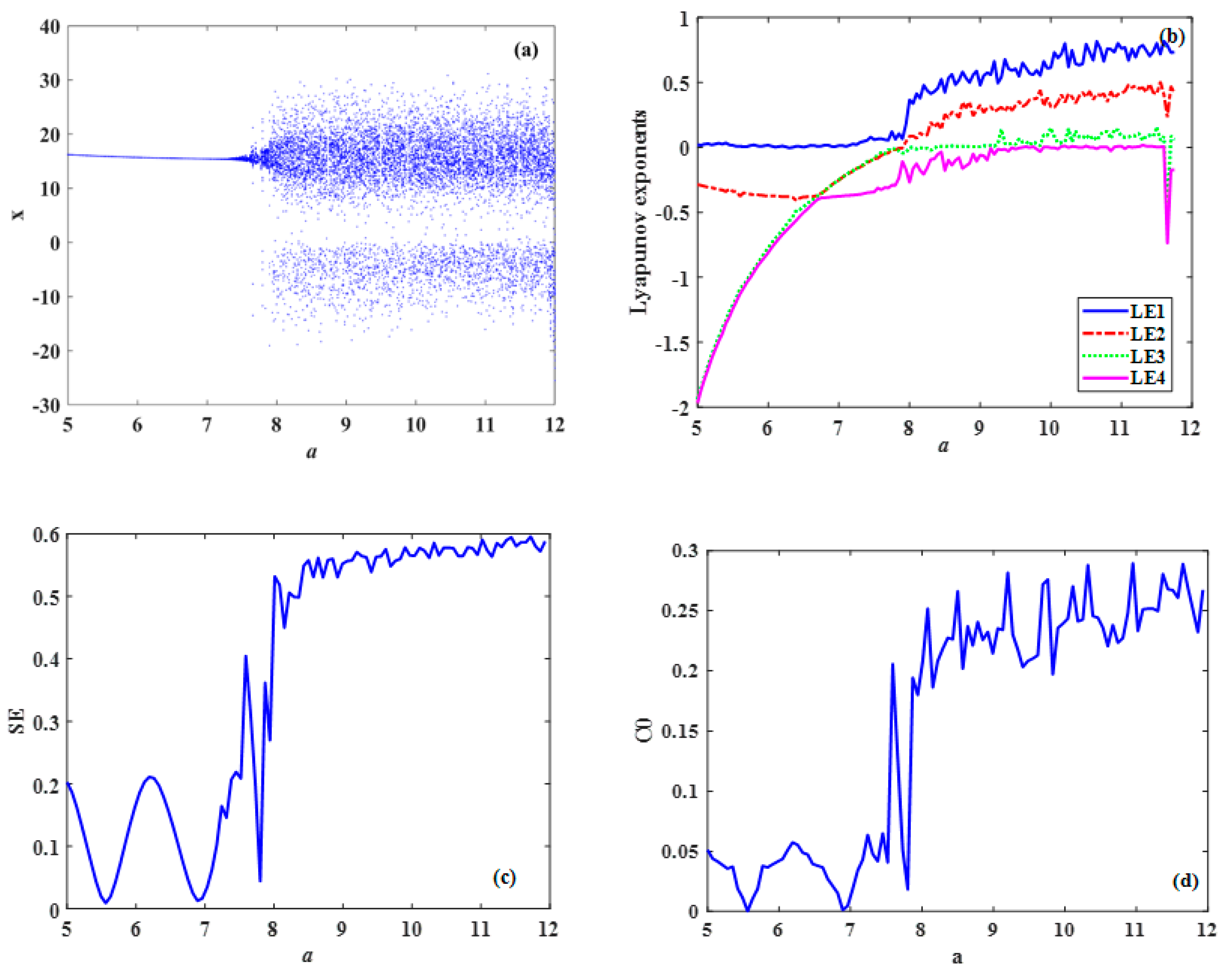
4.2. Parameter a Varying

Let q = 0.9, b = 8 3 , c = 28 , d = 1.3 , h = 1.78 , k 1 = 1 and k 2 = 4.8 ; then, vary a from 5 to 12 with a step size of 0.01. Let the initial value (x0,y0,z0,w0,u0) = (1,0.2,0.3,0.4,0.5). The bifurcation diagram, Lyapunov exponent and complexity with parameter a are shown in Figure 5.
From the bifurcation diagram, it can be seen that the system (6) is periodic under parameter a ∈ [5,8), and the maximum Lyapunov exponent of the corresponding system (6) is equal to 0. a ∈ [8,12]. System (6) is chaos; the maximum Lyapunov exponent is greater than 0, and the C0 and SE complexity is high, as shown in Figure 5c,d. a ∈ [8,12]. At some points in this interval, the system has three positive Lyapunov exponents, at which time the system complexity reaches the maximum, as shown in Figure 5b–d. In a five-dimensional chaotic system, it is rare to have three positive Lyapunov exponents. According to the preceding analysis, it is easy to find that the C0 and SE complexity and the maximum Lyapunov exponent results are consistent. In addition, the system complexity is also related to the number of positive Lyapunov exponents.

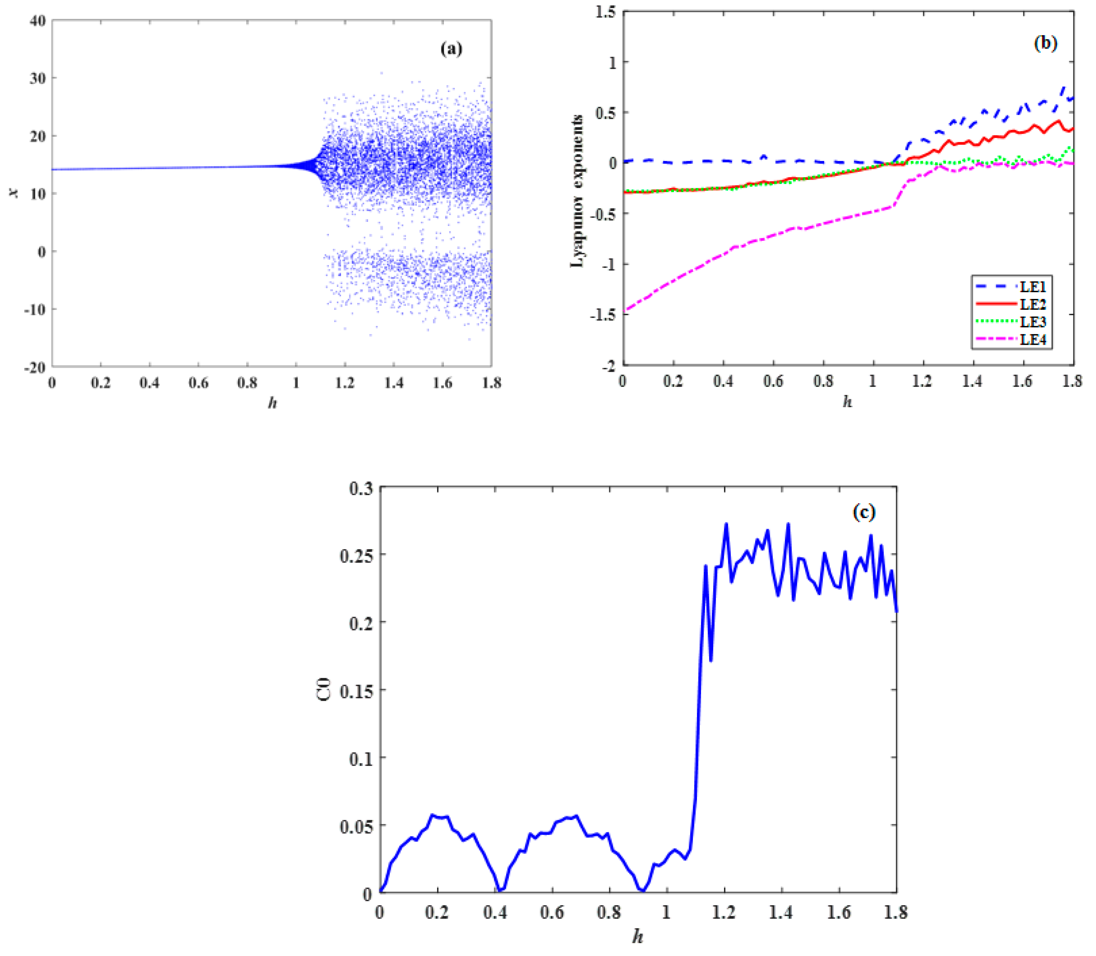
4.3. Varying Parameter h

Let there be fixed parameters a = 10 , b = 8 3 , c = 28 , d = 1.3 , k 1 = 1 , k 2 = 4.8 , and q = 0.9 . Let h [ 0 , 1.8 ] . The bifurcation diagram, Lyapunov exponent and complexity of system (6) are shown in Figure 6. It can be seen from the bifurcation diagram in Figure 6a that the h ∈ (0, 1.2) system (6) belongs to a periodic state. The maximum Lyapunov exponent corresponding to system (6) is equal to zero, and the C0 complexity of system (6) is about 0.05.
When h ( 1.18 , 1.8 ] , system (6) is in a chaotic state, and the maximum Lyapunov exponent corresponding to the interval of system (6) is greater than 0. When h = 1.6, the system has 3 positive Lyapunov exponents, and the complexity C0 of the system (6) is about 0.25. It can be seen from the change of parameter h that the bifurcation diagram of the system is basically consistent with the complexity of the system.

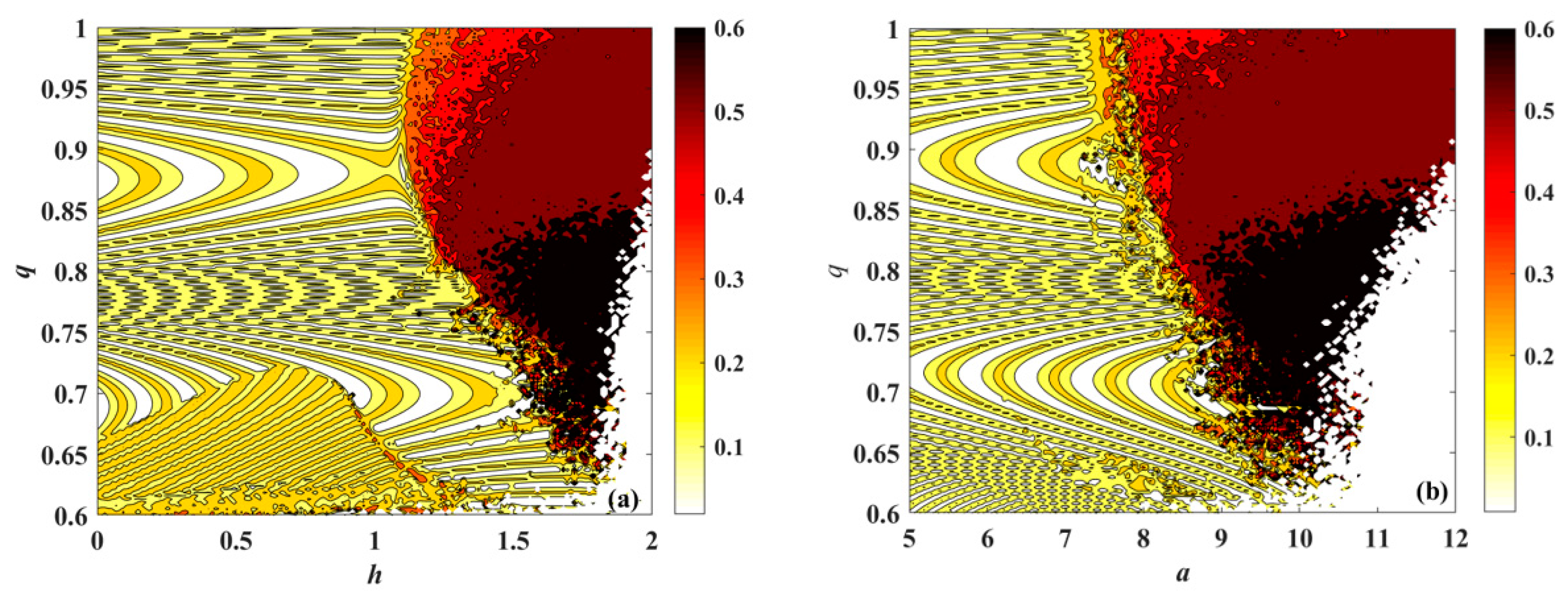
4.4. C0 Complexity Diagram

The C0 complexity diagram indicates the variation of the C0 complexity with changes in two parameters. Complexity is based on time series, and the maximum complexity is 1. This can help us choose the most suitable parameters in practical applications. h and q change as shown in Figure 7a, and a and q change as shown in Figure 7b. In Figure 7, different colors indicate different values of C0 complexity. Darker colors represent greater C0 complexity. When the system parameters h and a change, the smaller the q value, the greater the complexity (darker the color), which further shows that the fractional-order chaotic system is more complex than the integer-order chaotic system. This high-complexity area means that the system is chaotic or hyperchaotic; however, the complexity diagram cannot show details and is thus unable to distinguish the period from chaos.

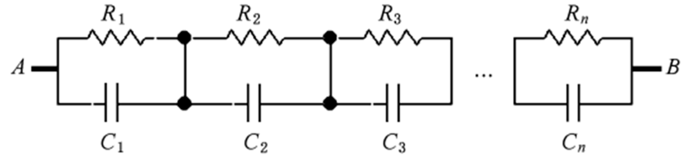
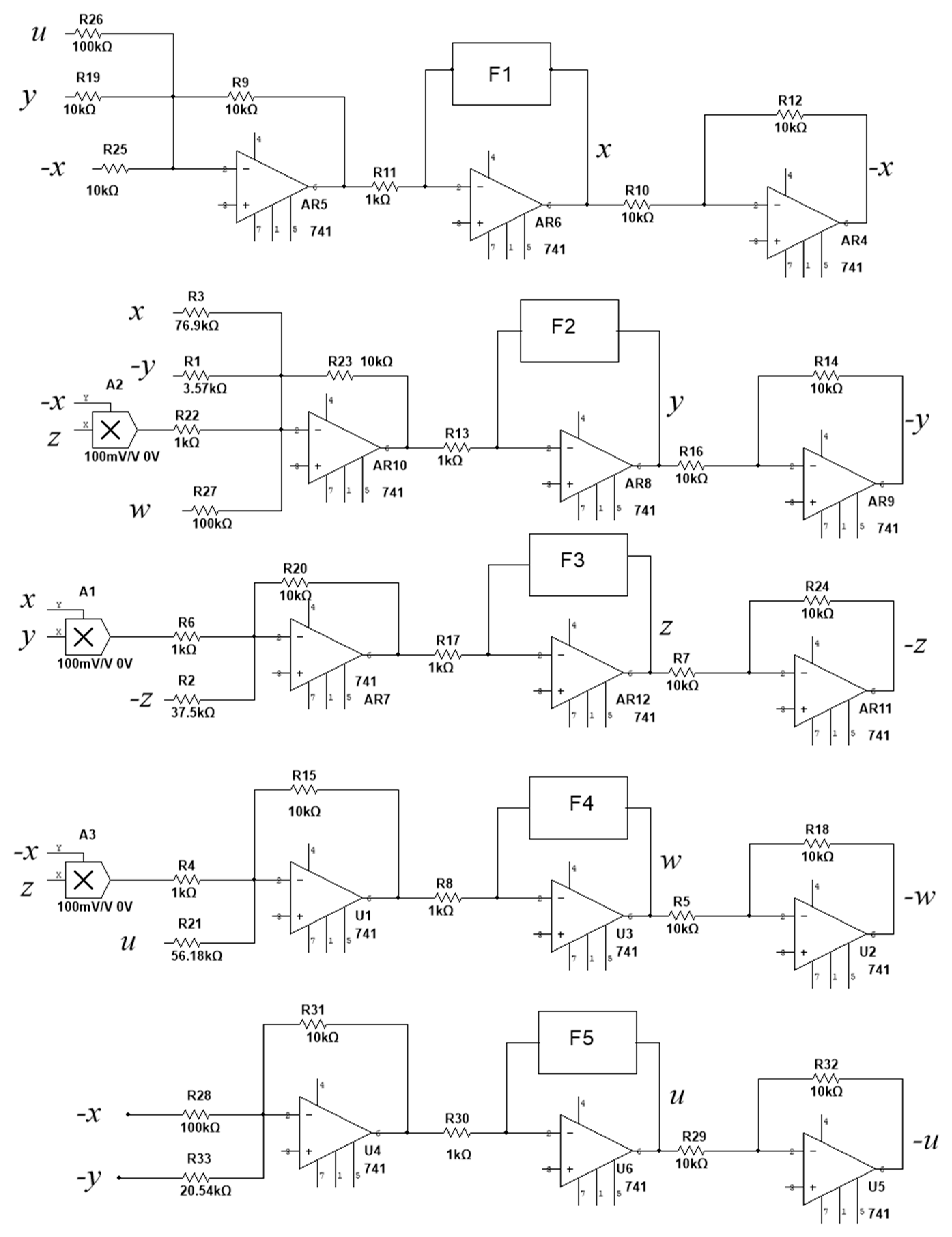
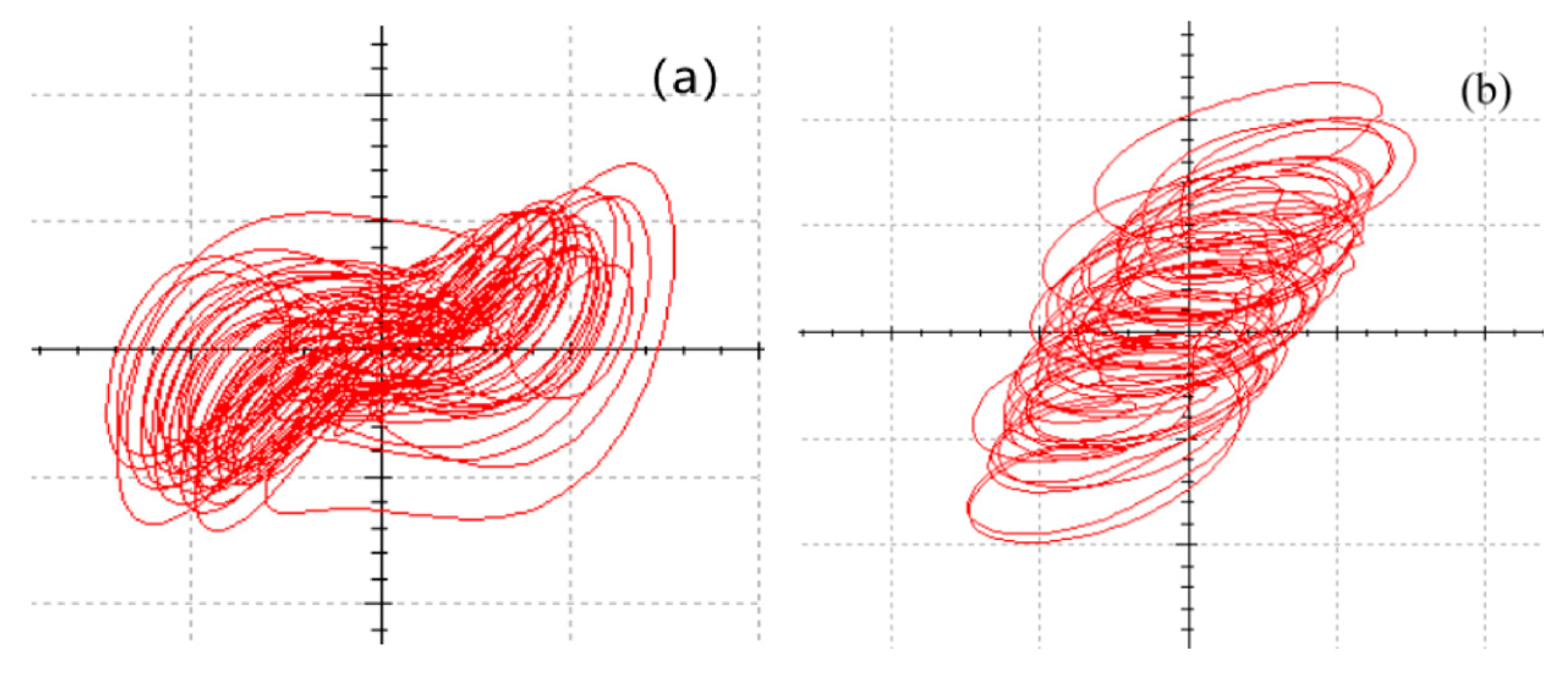
5. Design and Simulation of a Fractional-Order Circuit

For the design of fractional-order chaotic circuits, most of the circuits are designed with the order of 0.1~0.9. In this paper, the maximum frequency of the system is 100 Hz, and the error is 2 dB by using the method of reference [30,31]. The expansion formula of fractional order q (0.90~0.99) of the system is calculated as shown in Table 1.
According to the 0.90~0.99-order tension expansion and the circuit design method in references [32,33], the designed fractional-order circuit is shown in Figure 8. The resistance values of the corresponding order are shown in Table 2, and the capacitance values are shown in Table 3.
According to the dynamic equation of chaotic system (6), the circuit of fractional chaotic system (1) is designed, and the circuit schematic diagram is shown in Figure 9. Chaotic system (6) is realized by the modular circuits of resistors with different resistance values, capacitors with different capacitance values, operational amplifier LM741 and multipliers AD633 and 1 / s 0.96 . The working voltage of operational amplifier LM741 and multiplier AD633 is limited, so the system linearity is reduced to 0.1 times the original circuit design [31].
Multisim13 is used to simulate the designed analog circuit, and the horizontal axis is adjusted during the simulation process. The results are displayed in real-time on the oscilloscope, as shown in Figure 10.

6. Conclusions

In this paper, we focus on a class of 5D fractional-order hyperchaotic systems, use the Adomian decomposition method to approximate the solution of the system, and use bifurcation diagrams, Lyapunov exponent spectrum, SE complexity and C0 complexity to simulate and analyze the basic dynamic behavior of the system. Finally, based on the modular circuit design method, the circuit of a fractional-order chaotic system is designed, and the oscilloscope display results are consistent with the simulation results, which provide a basis for the circuit design and control of fractional-order electromechanical coupling systems.

Author Contributions

Conceptualization, T.L.; methodology, T.L. and H.F.; software, H.F.; validation, T.L. and H.F.; formal analysis, T.L.; investigation, H.F.; resources, T.L.; data curation, T.L.; writing—original draft preparation, H.F.; writing—review and editing, T.L.; visualization, T.L. and H.F.; supervision, T.L.; project administration, T.L. All authors have read and agreed to the published version of the manuscript.

Funding

This work was supported the Major Scientific and Technological Innovation Projects of Shandong Province (Grant No.2019JZZY010111), the Key Research and Development Plan of Shandong Province (Grant No.: 2019GGX104092), and the Science and Technology Plan Projects of Universities of Shandong Province (Grant No.: J18KA381).

Institutional Review Board Statement

Not applicable.

Informed Consent Statement

Not applicable.

Data Availability Statement

All datasets generated for this study are included in the article.

Conflicts of Interest

The authors declare no conflict of interest.

References

  1. Bolotin, K.I.; Ghahari, F.; Shulman, M.D.; Stormer, H.L.; Kim, P. Observation of the fractional quantum Hall effect in graphene. Nature 2009, 462, 196–199. [Google Scholar] [CrossRef] [PubMed] [Green Version]
  2. Tarasov, V.E.; Zaslavsky, G.M. Fractional dynamics of coupled oscillators with long-range interaction. Chaos Interdiscip. J. Nonlinear Sci. 2006, 16, 023110. [Google Scholar] [CrossRef] [PubMed] [Green Version]
  3. Agrawal, O.P. A general formulation and solution scheme for fractional optimal control problems. Nonlinear Dyn. 2004, 38, 323–337. [Google Scholar] [CrossRef]
  4. Torvik, P.J.; Bagley, R.L. On the appearance of the fractional derivative in the behavior of real materials. J. Appl. Mech. 1984, 51, 725–728. [Google Scholar] [CrossRef]
  5. Wang, Y.; Sun, K.; He, S.; Wang, H. Dynamics of fractional-order sinusoidally forced simplified Lorenz system and its synchronization. Eur. Phys. J. Spec. Topics 2014, 223, 1591–1600. [Google Scholar] [CrossRef]
  6. He, S.; Sun, K.; Wang, H. Complexity analysis and DSP implementation of the fractional-order Lorenz hyperchaotic system. Entropy 2015, 17, 8299–8311. [Google Scholar] [CrossRef] [Green Version]
  7. Chen, H.; Lei, T.; Lu, S.; Dai, W.; Qiu, L.; Zhong, L. Dynamics and Complexity Analysis of Fractional-Order Chaotic Systems with Line Equilibrium Based on Adomian Decomposition. Complexity 2020, 2020, 5710765. [Google Scholar] [CrossRef]
  8. Lei, T.; Mao, B.; Zhou, X.; Fu, H. Dynamics Analysis and Synchronous Control of Fractional-Order Entanglement Symmetrical Chaotic Systems. Symmetry 2021, 13, 1996. [Google Scholar] [CrossRef]
  9. He, S.; Natiq, H.; Banerjee, S.; Sun, K. Complexity and Chimera States in a Network of Fractional-Order Laser Systems. Symmetry 2021, 13, 341. [Google Scholar] [CrossRef]
  10. He, S.; Sun, K.; Wang, H.; Mei, X.; Sun, Y. Generalized synchronization of fractional-order hyperchaotic systems and its DSP implementation. Nonlinear Dyn. 2018, 92, 85–96. [Google Scholar] [CrossRef]
  11. Li, C.; Su, K.; Tong, Y.; Li, H. Robust synchronization for a class of fractional-order chaotic and hyperchaotic systems. Opt.-Int. J. Light Electron Opt. 2013, 124, 3242–3245. [Google Scholar] [CrossRef]
  12. He, J.; Lei, T.; Jiang, L. Sliding Mode Matrix-Projective Synchronization for Fractional-Order Neural Networks. J. Math. 2021, 2021, 4562392. [Google Scholar] [CrossRef]
  13. He, S.; Banerjee, S.; Yan, B. Chaos and symbol complexity in a conformable fractional-order memcapacitor system. Complexity 2018, 2018, 4140762. [Google Scholar] [CrossRef]
  14. Gorenflflo, R.; Mainardi, F. Fractal and Fractional Calculus in Continuum Mechanics; Springer: New York, NY, USA, 1997. [Google Scholar]
  15. Tavazoei, M.S.; Haeri, M. Unreliability of frequency-domain approximation in recognizing chaos in fractional-order systems. IET Signal Process. 2007, 1, 171–181. [Google Scholar] [CrossRef]
  16. Sun, H.H.; Abdelwahab, A.; Onaral, B. Linear approximation of transfer function with a pole of fractional power. IEEE Trans. Autom. Control 1984, 29, 441–444. [Google Scholar] [CrossRef]
  17. Deng, W. Short memory principle and a predictor–corrector approach for fractional differential equations. J. Comput. Appl. Math. 2007, 206, 174–188. [Google Scholar] [CrossRef] [Green Version]
  18. Diethelm, K.; Ford, N.J.; Freed, A.D. A predictor-corrector approach for the numerical solution of fractional differential equations. Nonlinear Dyn. 2002, 29, 3–22. [Google Scholar] [CrossRef]
  19. Adomian, G. A review of the decomposition method and some recent results for nonlinear equations. Math. Comput. Model. 1990, 13, 17–43. [Google Scholar] [CrossRef]
  20. Wang, H.H.; Sun, K.H.; He, S.B. Dynamic analysis and implementation of a digital signal processor of a fractional-order Lorenz–Stenflflo system based on the Adomian decomposition method. Phys. Scr. 2015, 90, 15206. [Google Scholar] [CrossRef]
  21. Peng, D.; Sun, K.H.; He, S.B.; Zhang, L.M.; Alamodi, A.O. Numerical analysis of a simplest fractional-order hyperchaotic system. Theor. Appl. Mech. Lett. 2019, 9, 220–228. [Google Scholar] [CrossRef]
  22. Fazzino, S.; Caponetto, R.; Patané, L. A new model of Hopfifield network with fractional-order neurons for parameter estimation. Nonlinear Dyn. 2021, 104, 2671–2685. [Google Scholar] [CrossRef]
  23. Zhang, H.; Sun, K.; He, S. A fractional-order ship power system with extreme multistability. Nonlinear Dyn. 2021, 106, 1027–1040. [Google Scholar] [CrossRef]
  24. Yan, B.; He, S. Dynamics and complexity analysis of the conformable fractional-order two-machine 269 interconnected power system. Math. Methods Appl. Sci. 2021, 44, 2439–2454. [Google Scholar] [CrossRef]
  25. He, S.; Sun, K.; Mei, X.; Yan, B.; Xu, S. Numerical analysis of a fractional-order chaotic system based on conformable fractional-order derivative. Eur. Phys. J. Plus 2017, 132, 1–11. [Google Scholar] [CrossRef]
  26. Shao-Bo, H.; Ke-Hui, S.; Hui-Hai, W. Solution of the fractional-order chaotic system based on Adomian decomposition algorithm and its complexity analysis. Acta Phys. Sin. 2014, 63, 58–65. [Google Scholar] [CrossRef]
  27. Yang, Q.; Chen, C. A 5D Hyperchaotic system with three positive Lyapunov exponents coined. Int. J. Bifurc. Chaos 2013, 23, 1350109. [Google Scholar] [CrossRef]
  28. Staniczenko, P.P.; Lee, C.F.; Jones, N.S. Rapidly detecting disorder in rhythmic biological signals: A spectral entropy measure to identify cardiac arrhythmias. Phys. Rev. 2009, 79, 011915. [Google Scholar] [CrossRef]
  29. En-hua, S.; Zhi-jie, C.; Fan-ji, G. Mathematical foundation of a new complexity measure. Appl. Math. Mech. 2005, 26, 1188–1196. [Google Scholar] [CrossRef]
  30. Wang, Z.; Lei, T.F.; Xi, X.J.; Sun, W. Fractional control and generalized synchronization for a nonlinear electromechanical chaotic system and its circuit simulation with Multisim. Turk. J. Electr. Eng. Comput. Sci. 2016, 24, 1502–1515. [Google Scholar] [CrossRef]
  31. Alattas, K.A.; Mostafaee, J.; Sambas, A.; Alanazi, A.K.; Mobayen, S.; Vu, M.T.; Zhilenkov, A. Nonsingular Integral-Type Dynamic Finite-Time Synchronization for Hyper-Chaotic Systems. Mathematics 2022, 10, 115. [Google Scholar] [CrossRef]
  32. Ahmad, W.M.; Sprott, J.C. Chaos in fractional-order autonomous nonlinear systems. Chaos Solitons Fractals 2003, 16, 339–351. [Google Scholar] [CrossRef] [Green Version]
  33. Chongxin, L. Theory and Application of Fractional Order Chaotic Circuits; Xi’an Jiaotong University Press: Xi’an, China, 2011. [Google Scholar]
Figure 1. Phase diagram in different projections of a fractional-order chaotic system. (a) Phase portraits in the x-u plane. (b) Phase portraits in the x-z plane. (c) Phase portraits in the x-y plane. (d) Phase portraits in the x-w plane.
Symmetry 14 00484 g001
Figure 2. Lyapunov exponents of the system (6). (a) Top four Lyapunov exponent spectra. (b) Fifth Lyapunov exponent.
Symmetry 14 00484 g002
Figure 3. Bifurcation diagram, Lyapunov exponent and complexity of the system (6) varying with q. (a) Bifurcation diagram. (b) Lyapunov exponents spectrum. (c) SE complexity. (d) C0 complexity.
Symmetry 14 00484 g003
Figure 4. Phase diagram and p-s plane of the system with q = 0.68. (a) Phase diagram. (b) The p-s plane.
Symmetry 14 00484 g004
Figure 5. Bifurcation diagram, Lyapunov exponent and complexity of the system (6) varying with a. (a) Bifurcation diagram. (b) Lyapunov exponents spectrum. (c) SE complexity. (d) C0 complexity.
Symmetry 14 00484 g005
Figure 6. Bifurcation diagram, Lyapunov exponent and complexity of the system (6) varying with h. (a) Bifurcation diagram. (b) Lyapunov exponents spectrum. (c) C0 complexity.
Symmetry 14 00484 g006
Figure 7. C0 complexity diagram. (a) Changes in q and h. (b) Chanes in a and q.
Symmetry 14 00484 g007
Figure 8. The module circuit of 1 / s q .
Symmetry 14 00484 g008
Figure 9. Circuit diagrams of system (6).
Symmetry 14 00484 g009
Figure 10. The oscilloscope display of system (6). (a) Phase portraits in the x-y plane. (b) Phase portraits in the x-w plane.
Symmetry 14 00484 g010
Table 1. Approximation formula of the bode plot for fractional order q (0.90 to 0.99) (error 2 dB).
q H ( s ) = 1 / s q
0.90 H ( s ) = 2.2675 ( s + 1.2915 ) ( s + 215.4435 ) ( s + 0.0129 ) ( s + 2.1544 ) ( s + 359.3814 )
0.91 H ( s ) = 2.3413 ( s + 2 . 1484 ) ( s + 594 . 4492 ) ( s + 0.0129 ) ( s + 3.5636 ) ( s + 986.041 )
0.92 H ( s ) = 2.4181 ( s + 4.0616 ) ( s + 2118.8 ) ( s + 0.0128 ) ( s + 6.7002 ) ( s + 3495.3 )
0.93 H ( s ) = 2.4982 ( s + 9.2187 ) ( s + 10886 ) ( s + 0.0128 ) ( s + 15.1267 ) ( s + 17862 )
0.94 H ( s ) = 2.5818 ( s + 27.5243 ) ( s + 96787 ) ( s + 0.0128 ) ( s + 44.9244 ) ( s + 157970 )
0.95 H ( s ) = 1.6436 ( s + 127.4275 ) ( s + 0.0127 ) ( s + 206.9138 )
0.96 H ( s ) = 1.7080 ( s + 1271.1 ) ( s + 0.0127 ) ( s + 2053.5 )
0.97 H ( s ) = 1.7753 ( s + 58852 ) ( s + 0.0127 ) ( s + 94612 )
0.98 H ( s ) = 1.8455 ( s + 126490000 ) ( s + 0.0126 ) ( s + 202360000 )
0.99 H ( s ) = 1.9188 ( s + 1.2619 × 10 18 ) ( s + 0.0126 ) ( s + 2.0092 × 10 18 )
Table 2. The module circuit of the resistor for fractional (0.90 to 0.99) (error 2 dB).
qR1R2R3
0.9062.84730.25300.0250
0.9165.80810.15740.0094
0.9269.33100.08630.00027
0.9372.45270.039320.00054
0.9475.70250.01366.3 × 10−6
0.9579.69840.00305
0.9683.69840.0030
0.9786.95277.1 × 10−6
0.9891.55353.4 × 10−9
0.9995.64343.5 × 10−19
Table 3. The module circuit of capacitors for fractional (0.90 to 0.99) (error 2 dB).
qC1C2C3
0.901.23151.83481.0983
0.911.17801.78181.0739
0.921.12681.73111.0493
0.931.07831.68131.0246
0.941.03201.63201.0000
0.950.98791.5837
0.960.94591.5366
0.970.90561.4903
0.980.86691.4452
0.990.82981.4012
Publisher’s Note: MDPI stays neutral with regard to jurisdictional claims in published maps and institutional affiliations.

