Characterizing the E⊗e Jahn–Teller Potential Energy Surfaces by Differential Geometry Tools

Abstract

The term ‘mathematical chemistry’ is mostly associated with applications of graph theory in topological issues of 3D chemical structures, thought of as a collection of atoms as dots and bonds as lines. We propose here new directions in this field, coming from the side of theoretical chemistry approached with modern computational tools. Possible challenges are proposed in using ancillary tools of differential geometry for examining the potential energy surfaces of certain specific structural prototypes. Concretely, we describe here the geodesics on the surfaces related to the potential energy functions of the so-called E⊗e Jahn–Teller effect, a spontaneous symmetry-breaking phenomenon also known as a case of conical intersection. To illustrate the case, first-principles (ab initio) quantum chemical calculations are performed on the cyclo-propenyl molecular radical C₃H₃.

1. Introduction

The Jahn–Teller effect [1] designates a class of molecular problems implying the quantum treatment of electrons and nuclei together with their mutual interactions, such aspects being of interest in specialized branches of the physics of chemistry [2,3]. The molecules are quantum objects, first of all due to their electrons, while the nuclei can often be approximated as classical charges fixed in space, in a manner defining the molecular geometry. This is the so-called Born–Oppenheimer approximation [4] quasi-generally used in applied molecular quantum mechanics, i.e., computational chemistry [5,6]. Jahn–Teller effects appear when the validity of the Born–Oppenheimer simplifying assumption breaks down. From a more general perspective, the quantum interplay of nuclei and electron movements is called vibronic coupling (which may occur beyond Jahn–Teller effect cases) [7], an equivalent of the electron–phonon term used in the language of solid-state electronic structures [8].

The Jahn–Teller theorem states that a non-linear molecule with a degenerate ground-state (i.e., a set of lowest levels with the same energy) undergoes spontaneous symmetry breaking manifested as a geometrical distortion of the molecular frame (displacement of the nuclei from their former high-symmetry arrangement), removing the initial degeneracy (arriving then at a single non-degenerate state with the lowest potential energy). In the sense of point group theory [9,10], the electronic states and the molecular displacements are spanning representations with a dimension greater than unity. The simplest case is the two-dimensional symmetry representation labeled E in various point groups. A prototypical Jahn–Teller effect is denoted E⊗e, having a doubly degenerate ground-state with E-type symmetry coupled with a set of distortions also having a two-fold nature denoted by the non-capitalized letter e.

For instance, an equilateral triangular molecule with the E ground term is not stable in the high-symmetry form, tending to distort in isosceles or scalene triangles [11,12]. A regular octahedron with the E ground term may tend to an elongated or compressed square bipyramid [13,14], or behave dynamically [15,16], with the distortion axis visiting the three pairs of opposite vertices. The graphical representation of the two energy surfaces originating from the E term as a function of the two variables defining the e-type nuclear coordinates (tuning the molecular geometry) obtains a shape suggestively named the Mexican hat (in the first order) or the tricorn (in second and higher perturbation orders), as will be detailed in the following.

Although well studied in various respects, the Jahn–Teller effects remain exotic to the public at large, being also associated with supplementary intricacies such as the Berry phase [17]. Here, we propose yet another perspective for characterizing a prototypical Jahn–Teller potential energy profile, the celebrated Mexican hat, in the frame of differential geometry. To the best of our knowledge, the Jahn–Teller model surfaces have yet to be submitted to the scrutiny of such concepts. A start on this exploratory new route is proposed in the following.

This work is an interdisciplinary endeavor continuing our previous studies in this line [18]. The presented problem lies at the interface of the theoretical chemistry [19,20,21,22] and differential geometry [23,24,25] specializations of the authors, throwing new light on the rather complicated issue of vibronic effects.

2. Methods

The analytic derivations and graphical representations were obtained with the Mathematica^TM computer algebra software [26,27]. More concretely, the data discussed in Section 3.2 were obtained with the function NDSolve for numerically solving differential equations, the outcome being represented with the Plot3D and ParametricPlot3D graphic routines. The data in Section 3.3 were handled in the Matlab–Octave environments [28,29], using fminsearch for fitting and surf for graphical rendering.

Quantum chemical calculations were performed with the General Atomic and Molecular Electronic Structure System (GAMESS) code [30,31] using the correlation-consistent polarized valence triple zeta (cc-pVTZ) basis [32]. The complete active space calculations were used in the state-average regime, considering the two terms that become degenerate in high-symmetry geometry. The high-symmetry geometry was optimized using the conical intersection procedures. The relaxed potential energy surface was scanned with the particular controls of the Hildebrandt type of coordinate input [33], allowing us to impose the desired C₃ moiety, while the positions of hydrogen atoms were the object of gradient optimization. The computed energy surface consisted of 275 points, each one the object of an input file running the above-mentioned constrained geometry optimization. The GAMESS input files were automatically generated with a Matlab–Octave script performing the conversion of polar coordinates of the e-type Jahn–Teller modes into molecular geometry, as defined specifically in Section 3.3, and writing out the necessary input keywords. The presented molecular geometry images were realized with the Molden software [34].

3. Results and Discussion

3.1. The E⊗e Potential Energy Surfaces in the Linear Coupling Model

We consider the simplest case, namely the prototype of the E⊗e effect under linear coupling spanning the so-called “Mexican hat” potential energy surface. The coupled vibrational–electronic problem is, of course, an issue of wave-mechanics, but we ignore some of the details, taking directly the equations of the related surfaces [2,3] and proceeding to their analysis in terms of geodesics and curvature. Thus, we start concisely with the effective form of the equations defining the simplest E⊗e problem, the energy of the mentioned E states being eigenvalues of the following Hamiltonian matrix:

$$H_{E\otimes e }=\left(\begin{array}{cc}\frac{1}{2}K{\rho }^2& V\rho \\ V\rho & \frac{1}{2}K{\rho }^2\end{array}\right)$$

(1)

In the physical sense, K has the meaning of a force constant when the system is stressed along the ρ coordinate, while V, the first-order vibronic parameter, measures the strength of the coupling between the initially degenerate (equivalent) states. The e-type coordinates can be expressed in the polar format by ρ and φ, the above matrix being independent of the angular variable. The eigenvalues are:

$$e_{\pm }\left(\rho \right)=\frac{1}{2}K{\rho }^2\pm V\rho ,$$

(2)

being expressible in the unified form e(ρ) ≡ e₋(ρ) or e(ρ) ≡ e₊(ρ) if we conventionally allow the radial coordinate to take negative values. In this system, we have axial symmetry, which allows for the use of the idea of a rotational surface. The points of the surface can be described as the following set of coordinates:

$$\epsilon \left(\rho ,\phi \right)=\left\{\rho \cdot \cos \left(\phi \right),\rho \cdot \sin \left(\phi \right),e\left(\rho \right)\right\}.$$

(3)

For the concepts and formulae used in the further expansion, we refer the reader to the do Carmo monograph [35]. The metric is defined by the scalar products in the following manner:

$$g_{11}=\langle \frac{\partial \epsilon }{\partial \rho },\frac{\partial \epsilon }{\partial \rho }\rangle =\cos {\left(\phi \right)}^2+\sin {\left(\phi \right)}^2+{\left(K\rho +V\right)}^2=1+{\left(K\rho +V\right)}^2,$$

(4a)

$$g_{12}=g_{21}=\langle \frac{\partial \epsilon }{\partial \rho },\frac{\partial \epsilon }{\partial \phi }\rangle =-\rho \cdot \cos \left(\phi \right)\sin \left(\phi \right)+\rho \cdot \cos \left(\phi \right)\sin \left(\phi \right)=0,$$

(4b)

$$g_{22}=\langle \frac{\partial \epsilon }{\partial \phi },\frac{\partial \epsilon }{\partial \phi }\rangle ={\rho }^2\cos \left(\phi \right)+{\rho }^2\sin \left(\phi \right)={\rho }^2.$$

(4c)

Denoting by G the matrix with the above elements, one prepares its inverse in order to obtain the $g^{ij}$ = (G⁻¹)_ij elements. It follows that:

$$g^{11}=\frac{1}{1+e_{\rho }^{\prime }{}^2}=\frac{1}{1+{\left(K\rho +V\right)}^2},$$

(5a)

$$g^{12}=g^{21}=0,$$

(5b)

$$g^{22}=\frac{1}{{\rho }^2}.$$

(5c)

The Christoffel symbols in the given case are:

$${\mathsf{\Gamma }}_{ij}^k=\frac{1}{2}\left\{g^{k1}\left(\frac{\partial g_{1i}}{\partial {\zeta }^j}+\frac{\partial g_{1j}}{\partial {\zeta }^i}-\frac{\partial g_{ij}}{\partial {\zeta }^1}\right)+g^{k2}\left(\frac{\partial g_{2i}}{\partial {\zeta }^j}+\frac{\partial g_{2j}}{\partial {\zeta }^i}-\frac{\partial g_{ij}}{\partial {\zeta }^2}\right)\right\},$$

(6)

where $i,j,k\in \left\{1,2\right\}$ and $\rho ={\zeta }^1$, $\phi ={\zeta }^2$. By straightforward calculations, one obtains:

$${\mathsf{\Gamma }}_{11}^1=\frac{e_{\rho }^{\prime }{e}_{\rho }^{″}}{1+e_{\rho }^{\prime }{}^2}=\frac{K\left(K\rho +V\right)}{1+{\left(K\rho +V\right)}^2},$$

(7a)

$${\mathsf{\Gamma }}_{12}^1={\mathsf{\Gamma }}_{21}^1=0,$$

(7b)

$${\mathsf{\Gamma }}_{22}^1=-\frac{\rho }{1+e_{\rho }^{\prime }{}^2}=\frac{-\rho }{1+{\left(K\rho +V\right)}^2},$$

(7c)

$${\mathsf{\Gamma }}_{11}^2={\mathsf{\Gamma }}_{22}^2=0,$$

(7d)

$${\mathsf{\Gamma }}_{12}^2={\mathsf{\Gamma }}_{21}^2=\frac{1}{\rho } .$$

(7e)

The equations of geodesics on this surface are:

$${\ddot{\zeta }}^1+{\mathsf{\Gamma }}_{11}^1{\left({\dot{\zeta }}^1\right)}^2+2{\mathsf{\Gamma }}_{12}^1\left({\dot{\zeta }}^1\right)\left({\dot{\zeta }}^2\right)+{\mathsf{\Gamma }}_{22}^1{\left({\dot{\zeta }}^2\right)}^2=0,$$

(8a)

$${\ddot{\zeta }}^2+{\mathsf{\Gamma }}_{11}^2{\left({\dot{\zeta }}^1\right)}^2+2{\mathsf{\Gamma }}_{12}^2\left({\dot{\zeta }}^1\right)\left({\dot{\zeta }}^2\right)+{\mathsf{\Gamma }}_{22}^2{\left({\dot{\zeta }}^2\right)}^2=0,$$

(8b)

where the dot and double-dot upper-scripts denote the first and second derivatives, respectively, with respect to an evolution parameter (say, t):

$$\ddot{\rho }+\frac{e_{\rho }^{\prime }{e}_{\rho }^{″}}{1+e_{\rho }^{\prime }{}^2}{\left(\dot{\rho }\right)}^2-\frac{\rho }{1+e_{\rho }^{\prime }{}^2}{\left(\dot{\phi }\right)}^2=0,$$

(9a)

$$\ddot{\phi }+\frac{2}{\rho }\dot{\rho }\dot{\phi }=0.$$

(9b)

Rewritten with the above defined parameters, Equation (9a) turns into:

$$\ddot{\rho }+\frac{K\left(K\rho +V\right)}{1+{\left(K\rho +V\right)}^2}{\dot{\rho }}^2-\frac{\rho }{1+{\left(K\rho +V\right)}^2}{\dot{\phi }}^2=0.$$

(10)

On the other hand, geodesic Equation (9b) is related to the axial symmetry of the problem. Let us introduce $\omega =\dot{\phi }$, having the meaning of angular velocity, and subsequently perform certain rearrangements:

$$\dot{\frac{\omega }{\omega }}+2\frac{\dot{\rho }}{\rho }=0,$$

(11a)

$$\frac{d}{dt}\left(\ln \left(\omega \right)+\ln \left({\rho }^2\right)\right)=\frac{d}{dt}\ln \left(\omega {\rho }^2\right)=0.$$

(11b)

The last equality is nothing other than the conservation of angular momentum. By rescaling conventions, we eliminated the explicit factor of mass that appears in the physical definition of this quantity. In our circumstance, we retain the conservation of the product:

$${\rho }^2\omega ={\rho }^2\dot{\phi }=L=const.$$

(12)

This quantity is settled by the initial conditions of the differential equations.

Replacing the last equality in Equation (10), one obtains:

$$\ddot{\rho }+\frac{K\left(K\rho +V\right)}{1+{\left(K\rho +V\right)}^2}{\left(\dot{\rho }\right)}^2-\frac{L^2}{\left(1+{\left(K\rho +V\right)}^2\right){\rho }^3 }=0.$$

(13)

The problem is formally reduced to a one-variable second-order differential equation. Except for the L = 0 case, it becomes invalid at ρ = 0, such a singularity being physically forbidden for a particle in circular motion because it would imply an infinite angular velocity. In other words, a general geodesic cannot touch the radial origin.

To the best of our knowledge, general analytic solutions are not available, confining the discussion to numeric illustrations suggesting the patterns of geodesics placed in different areas of the coupled surfaces. In this view, we will consider conventional parameters and inspect the different types of geodesic curves.

3.2. Illustrating Geodesic Patterns on the “Mexican Hat” and Conical Intersection Surfaces

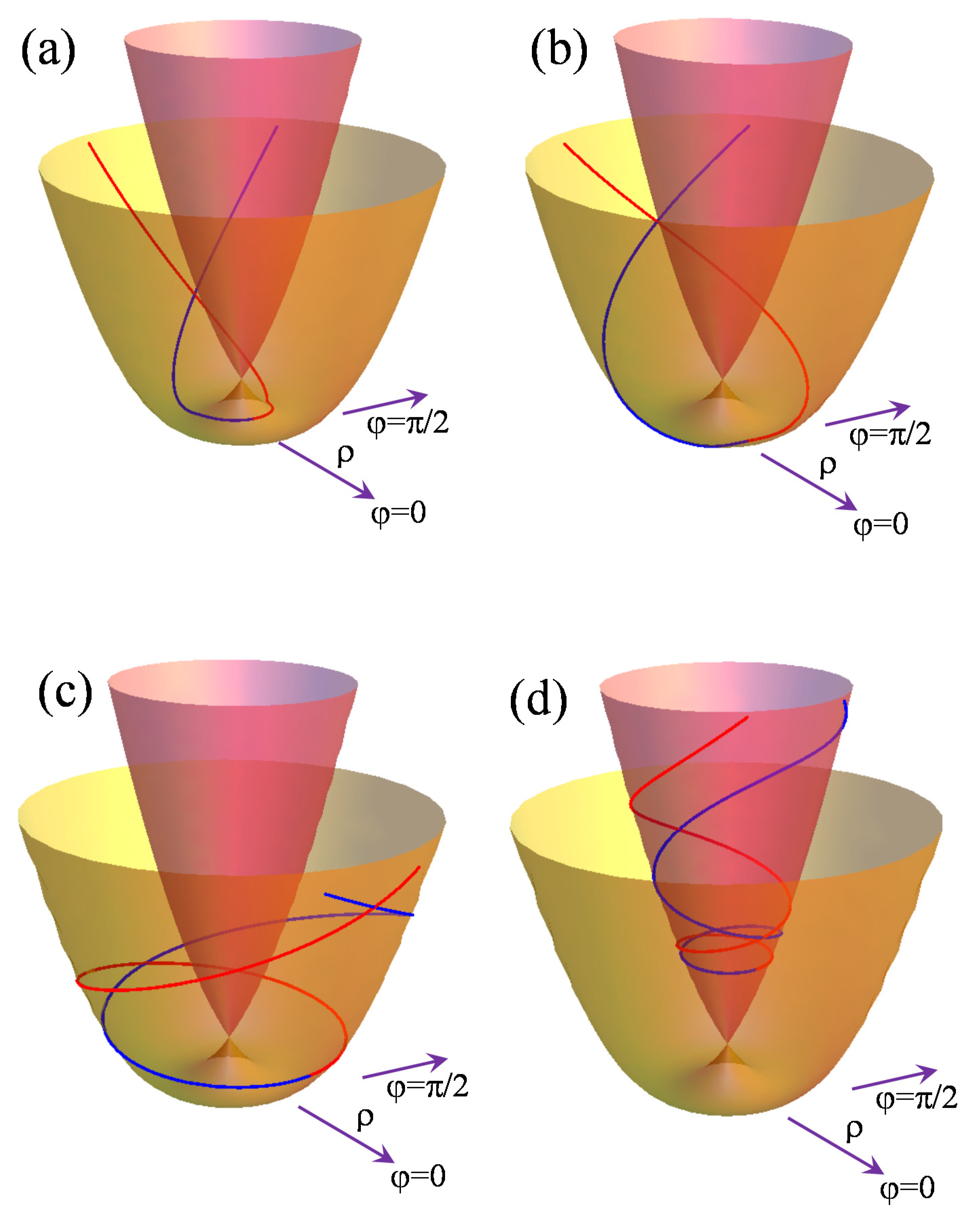
Figure 1 shows the general shape of the E⊗e problem. One may observe a composed surface, with the lower sheet having the minimum and the upper one having a steep slope everywhere. The two surfaces meet at the ρ = 0 degeneracy point. In this vicinity, the first-order term predominates, indicating another name given to such a topological pattern, namely a conical intersection [36,37]. This sort of crossing may also occur in other instances than the nominal Jahn–Teller effect, but it also has vibronic origins. The upper surface corresponds to the e₊(ρ) solution in Equation (2), being depicted with darker (violet) coloring in Figure 1, while the lowest sheet e₋(ρ) is drawn in a lighter color (yellow). The e₋(ρ) surface has a circular trough at the the ρ_min = V/K radius. With a certain scaling and cropping in the graphical representation of the surfaces, a certain resemblance to a Mexican hat can be observed, the E⊗e profile also being called this name. In our vertically elongated scaling, the “Mexican hat” name, as figure of speech, is not so obvious, but this is an irrelevant aspect.

The frames of Figure 1 illustrate qualitatively distinct placements of point P crossed by geodesics obeying the ${\dot{\rho }}_P=0$ initial condition in the corresponding differential equations. The initial polar coordinate is set to φ_P = 0, other arbitrary values being obtainable by the rotation with φ_P of the presented figures around the vertical axis.

The panels (a–c) explore the curves on the lower e₋(ρ) surface, produced with P at the respective smaller, equal, and larger radial coordinates, in comparison to the radius ρ_min of the minimum trough. Strictly speaking, the non-null initial condition due to the first-order derivative of the angular coordinate determines only one half of the geodesic line evolving in the clockwise or anti-clockwise direction with respect to P’s origin depending on the ${\dot{\phi }}_P>0$ or ${\dot{\phi }}_P$ < 0 case. We represented these halves in different colors, their meeting marking the starting point. In the discussed ${\dot{\rho }}_P=0$ situation, the geodesic halves modulated by the sign of ${\dot{\phi }}_P$ are symmetrical with respect to a mirror plane passing through the point P and the vertical axis at ρ = 0. The two branches of the geodesic spiral on the surface, crossing each other at polar coordinates equal to those of the initial point φ = φ_P and, on the diametrically opposed side, φ = φ_P + π. For the starting points on the upper surface (see panel d), e₊(ρ), and for the ones placed on the lower surface, e₋(ρ), after the minimum radius (see panels b and c), ρ_P ≥ ρ_min, the curves evolve upwards at elevations higher than the initial point e_±(ρ) > e_±(ρ_P).

For a point on the lower sheet, e₋(ρ), comprised of the origin and radius of the minimum trough, 0< ρ_P < ρ_min (see panel a), the geodesic goes first toward the minimum and then starts spiraling upward after crossing the valley. The rotation of the geodesics on the surfaces around the ρ = 0 vertical axis can be assigned to the positive curvature of the e_±(ρ) surfaces with respect to the ρ coordinate. This situation tells us that, in the long term, the geodesics cannot be interpreted with the intuition of the shortest path between two points because the cycling imposes lengthier routes than when drawing a curve with a monotonous variation in the angular parameter between the φ_P and φ_Q values of the generally distant P and Q references placed on the same geodesic. In turn, the minimum path interpretation holds in the infinitesimal sense of Q’s arrival occurring in the vicinity of P’s starting point.

Another special geodesic equation is the ${\dot{\phi }}_P=0$ case, i.e., a movement without an angular impetus, that actually keeps the angular coordinate constant along the curve φ = φ_P. This is the trivial case of the geodesic and is defined as the intersection of the e_±(ρ) surfaces with the vertical plane containing the ρ = 0 axis and the initial P point. These are the analogs of meridians, which are geodesics on the sphere. In turn the circles defined at a constant radial parameter ρ = ρ_P, are not allowed to be geodesics in similar manner to a globe in which parallels other than the equator do not fulfill the underlying equations.

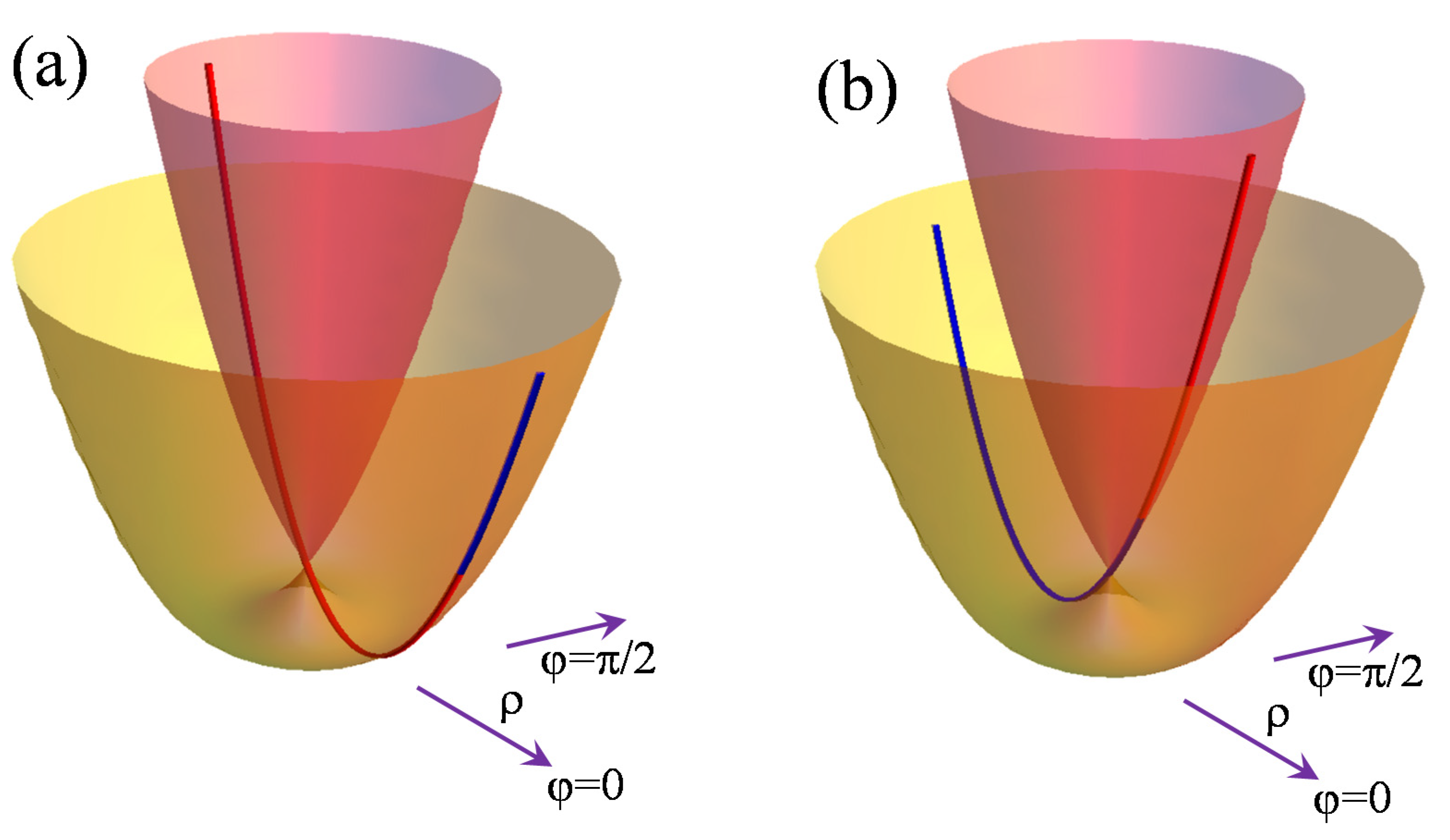
Figure 2 presents examples of solutions based on the ${\dot{\phi }}_P=0$ initial condition. One can observe that the curve continues on the other surface. If the starting point P is on the e_{_}(ρ) sheet, as in panel (a), it crosses the degeneracy at ρ = 0 and goes onto the e₊(ρ) surface. Vice versa, as shown in panel (b), it can pass from e₊(ρ) to e₋(ρ), the different colors of the curve branches helping us to visually locate the initial point at their confluence. Actually, in this situation, the geodesics are parabolas with the minimum located at the ρ_min contained in the plane defined by the vertical ρ = 0 axis and the point P.

The degeneracy crossing indicates the above-suggested perspective of a unified description of the reunion of the surfaces as a single object. Formally, this is realized by choosing only one of the equalities shown in Equation (2), say e(ρ) = e₋(ρ), the lower surface resulting then for ρ > 0 and the upper one being accounted for with an enforced negative ρ having e₊(ρ) = e(−ρ) = e_{_}(−ρ). Accepting such a non-standard convention is not essential to the discussion, but it helps us to deal with the inter-surface evolution of the particular meridian-like geodesics. In turn, in the above-mentioned case, as well as in the cases discussed below, with a non-null initial angular derivative ${\dot{\phi }}_P\ne 0$ the geodesics are not allowed to either touch the ρ conical intersection or to pass through onto the companion surface. This is determined by the avoidance of a singularity in the last term of Equation (13), or, in other words, by the physical denial of infinite angular momentum in the conservation law from (12).

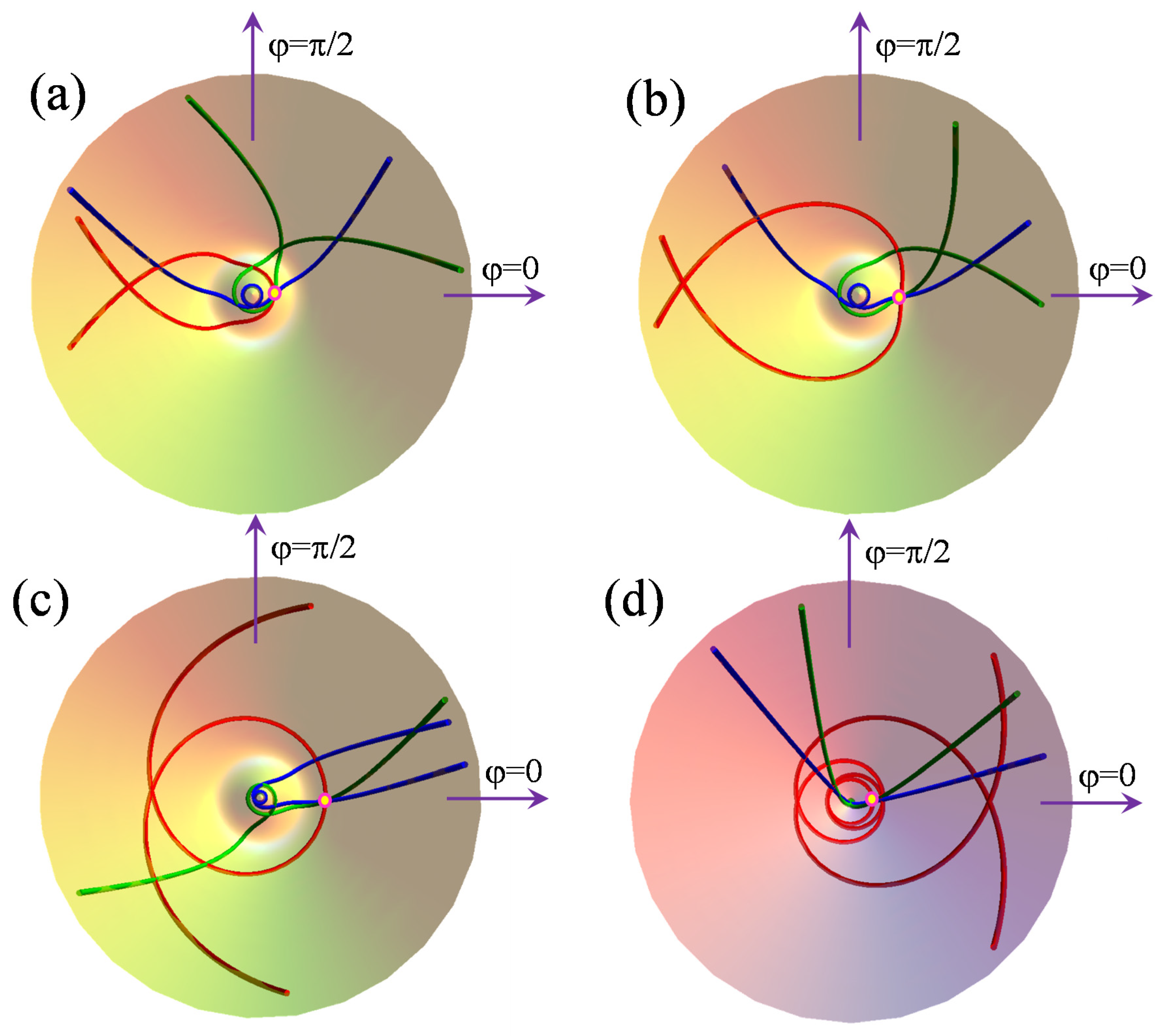
Figure 3 illustrates the situation of geodesics with non-null initial derivatives with respect to both the radial and angular variables (green and blue lines, respectively). However, for the sake of comparison, the particular situation of a null initial radial derivative was added (red geodesics). The blue line has a larger starting radial derivative than the green one (at the same angular value).

One may notice that the geodesics with the $\left|{\dot{\rho }}_P\right|\ne 0$ initial condition are not symmetric with respect to the initial point in the sense that the halves going in opposite directions from P are not identical, as is the case for ${\dot{\rho }}_P=0$. However, ignoring the starting point, each geodesic admits a symmetry plane where the condition ${\dot{\rho }}_Q=0$ is reached at the point Q. A geodesic has one unique point obeying the ${\dot{\rho }}_Q=0$ condition. At the same time, any arbitrary point P is passed by an infinite family of geodesics obtainable by tuning the local angle of the curves with respect to the particular reference with ${\dot{\rho }}_Q=0$. This angle is determined by the sign and magnitude of the ratio of the ${\rho }_P{\dot{\phi }}_P$ and ${\dot{\rho }}_P$ initial conditions. The ${\rho }_P$ factor was included in order to convert the angular derivative to the dimension of the radial one, akin to the physical meaning of the linear impulse.

On the lower surface, e₋(ρ), the geodesic has a part that approaches an orbit near the conical intersection. The larger the initial radial derivative, the closer the loop comes to the conical intersection, as seen in frames (a) and (b) in Figure 3, where the blue line climbs to a smaller radius and performs a complete cycle around the conical intersection, while the green one escapes before completing a cycle. Both branches evolve, in the long term, towards the upper part of e_{_}(ρ) at ρ > ρ_min. In the frames (c) and (d), both the blue and green lines perform a tour of the conical intersection, although, in the (d) panel, corresponding to the point P on the e₊(ρ) sheet, this is not easily visible because of the small radius near the conical point.

We refrain from adopting a classical mechanics explanation since the Jahn–Teller surface is a quantum object, but one may suggest that the cases (c) and (d) can be compared with the free fall from higher potential energies. Then, the line behaves analogously to one having a larger amount of momentum that allows for one or more circles at smaller radii. As discussed in the cases from Figure 1, the more general instances from Figure 3 do not allow a geodesic to escape the surface of the starting point, e₊(ρ) or e₋(ρ), this fact being possible only in the particular condition shown in Figure 2.

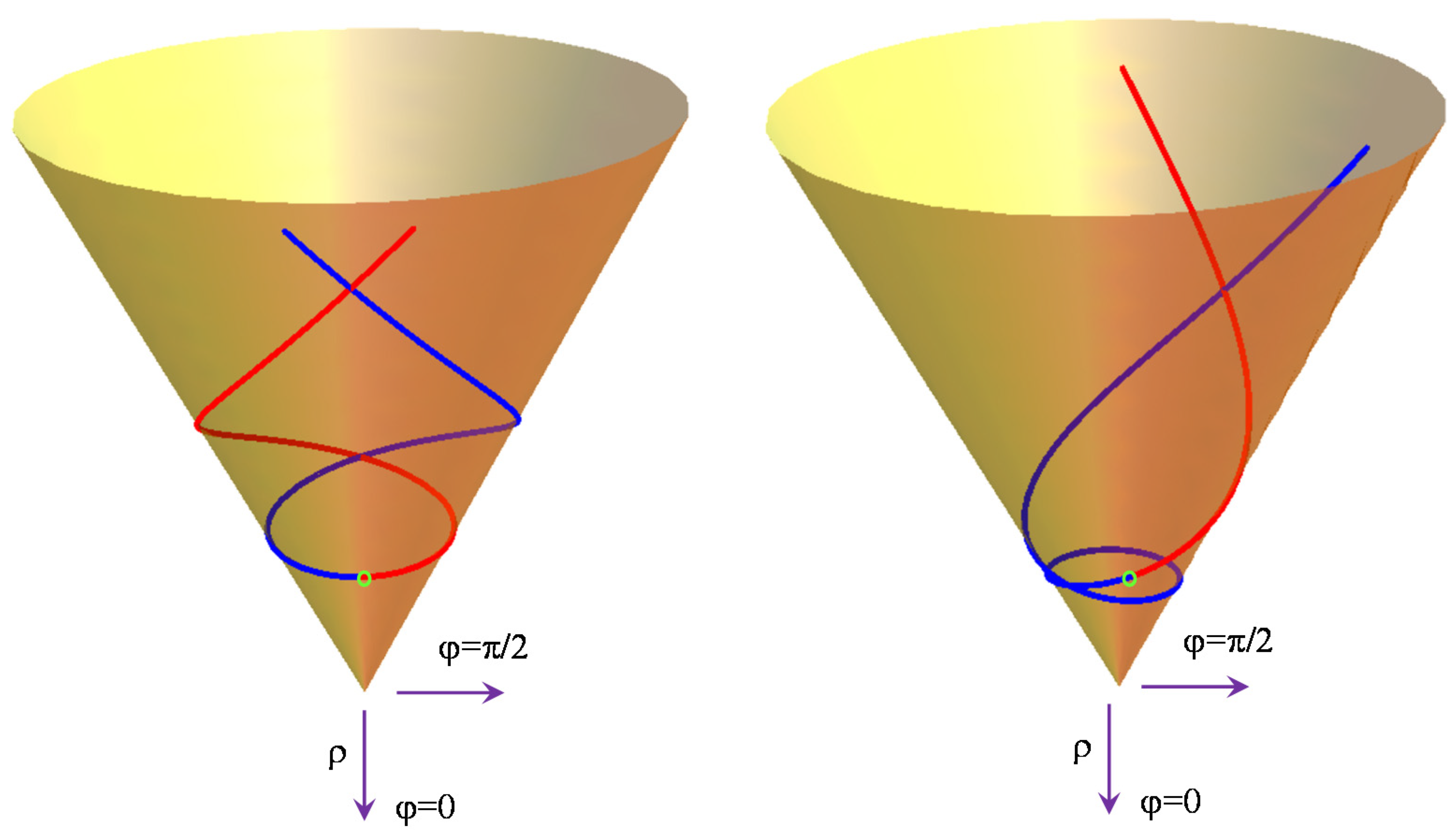
In the vicinity of the crossing point, both surfaces are approximated by cones with shared vertices. As pointed out previously, for this reason, in computational chemistry, this pattern is known as a conical intersection [34,35]. The equations for the cone and their geodesics can be derived if we impose K = 0 in the above formulas, i.e., e_±(ρ) = ±V ρ. Note that a cone is obtained if we take the half-difference of the eigenvalues: V ρ = (e₊(ρ) − e₋(ρ))/2.

In this simplified hypothesis, one may find analytical expressions for geodesics based on the fact that a cone can be presented as an isometric transformation of the plane (both surfaces have zero Gauss curvature); thus, any straight line in the initial plane is mapped onto a geodesic on the cone surface (see pages 246–247 in reference [35] and page 250 in [38]). In a parametric dependence on t, the cone geodesics starting from the point ρ₀ = r₀, φ₀ = 0, with the initial gradients $\dot{\rho }=r_0{p}_0\sin \left(u_0\right) /\sqrt{V^2+1}$ and $\dot{\phi }=p_0\cos \left(u_0\right)$, can be ascribed as follows:

$$\left\{r\left(t\right)\cdot \cos \left(\alpha \left(t\right)\right),r\left(t\right)\cdot \sin \left(\alpha \left(t\right)\right),V\cdot r\left(t\right)\right\},$$

(14)

where

$$r\left(t\right)=\sqrt{r_0^2+\frac{t^2\sqrt{V^2+1}+2r_{0}t\cdot \sin \left(u_0\right)}{V^2+1}},$$

(15a)

$$\alpha \left(t\right)=\sqrt{V^2+1}\cdot \mathrm{ArcTan}\left(\frac{t\cdot \cos \left(u_0\right)}{r_0\sqrt{V^2+1}+t\cdot \sin \left(u_0\right)}\right).$$

(15b)

One may observe that we used the conventional angular value u₀ to define a ratio between the linear tangential and radial velocities if the evolution parameter t is formally regarded as time.

The in-plane line related by isometry to the cone geodesics is:

$$\left\{\sqrt{V^2+1}+\cos \left(u_0\right)\cdot t,\sin \left(u_0\right)\cdot t,0\right\}.$$

(16)

We checked that the numeric solutions of the generic differential Equations (9) and (10) with the above initial conditions render the same curves as the analytical ones from Equations (14) and (15). The t > 0 and t < 0 branches are related by a sign swap in the initial derivatives (represented in red and blue, respectively, in Figure 4).

3.3. Quantum Chemical Calculation of the Jahn–Teller Effect in Triangular Molecular Systems

In this section, we aim to make concrete the E⊗e effect by state-of-the art calculations on an illustrative example. The simplest molecule imaginable for such a goal is the tri-hydrogen H₃. However, although it presents a conical intersection, the potential energy surface of H₃ does not show bonded minima [39,40], the system being prone to rapid dissociation in the molecular and atomic hydrogen H₂ + H, or to ionization, the H₃⁺ cation being a well-known molecule in the interstellar space [41]. Then, the next molecule on the simplicity scale would be the cyclo-propenyl radical C₃H₃. This molecule can be described as a triangle composed of carbon atoms bordered by a triangle composed of hydrogens bonded to carbons. According to chemical intuition, the Jahn–Teller effect is due to the so-called π electrons on the C₃ unit, the H₃ moiety just following the distortion of the carbon frame.

This radical is an intermediate in combustion processes [42]. Early electron spin resonance measurements proved the distortions to be due to the Jahn–Teller effect [43,44], and this finding was corroborated by similar conclusions from nuclear magnetic resonance spectra [45]. The first approaches to distortion effects in the cyclo-propenyl radical were put in the heuristic key of the so-called antiaromaticity [46] and were limited to the rather rudimentary calculation procedures available at the dawn of computational chemistry [47,48]. The studies were continuously re-enacted as progress was made in the calculation methods, retrieving the same qualitative and semi-quantitative conclusions [49,50]. The most recent and deep study of the C₃H₃ radical [51] used highly rated computational methods, the so-called coupled cluster routines [52], which, although not suited for multi-configurational and degenerate wave functions, are good at tackling the optimal distorted molecular geometries at the energy minima of the Jahn–Teller problem at hand.

Here, we performed Complete Active Space Self-Consistent Field (CASSCF) [53,54] calculations consisting of three electrons in three orbitals corresponding to the π subsystem of the planar molecule. A comprehensive modern study [55], carried out with accurate multi-configurational computations, treated in detail the Jahn–Teller and pseudo Jahn–Teller effects in the cyclo-propenyl radical and anion, outlining potential energy curves. However, full potential energy surfaces representing the ab initio complete mapping of the E⊗e problem in C₃H₃ have not been presented previously.

The upper part of Figure 5 shows the geometry of the unstable equilateral triangle, optimized in a conical intersection CASSCF procedure, along with the isosceles geometry stabilized as energy minimum. The change in bond lengths is not very large, but clearly illustrates that the stabilization can be interpreted as the formation of a simple C-C bond in concert with the delocalization of a double bond over two equal carbon–carbon lines.

The degenerate ground-state named previously, E, in a generic manner is, more precisely, a ²E″ term in the case of the π-type electronic system of the cyclo-propenyl in the D_3h symmetry point group. The molecular term has the same symmetry as those of the singly occupied degenerate orbital ascribed conventionally the non-capitalized label e″ (see the scheme in the left-bottom part of Figure 5). The double degeneracy of the ²E″ state comes from the two equivalent possibilities to place the unpaired electron in the two lodges of the e″ orbital set. One may see in the qualitative scheme shown in the lower part of Figure 5 that the distortion leads to the removal of orbital degeneracy (energy equivalence) in the e″ orbitals. The stable molecular geometry is an isosceles triangle with one elongated edge, the frontier orbital having the a₂ representation that gives rise to the corresponding ²A₂ ground state in the C_2v point group.

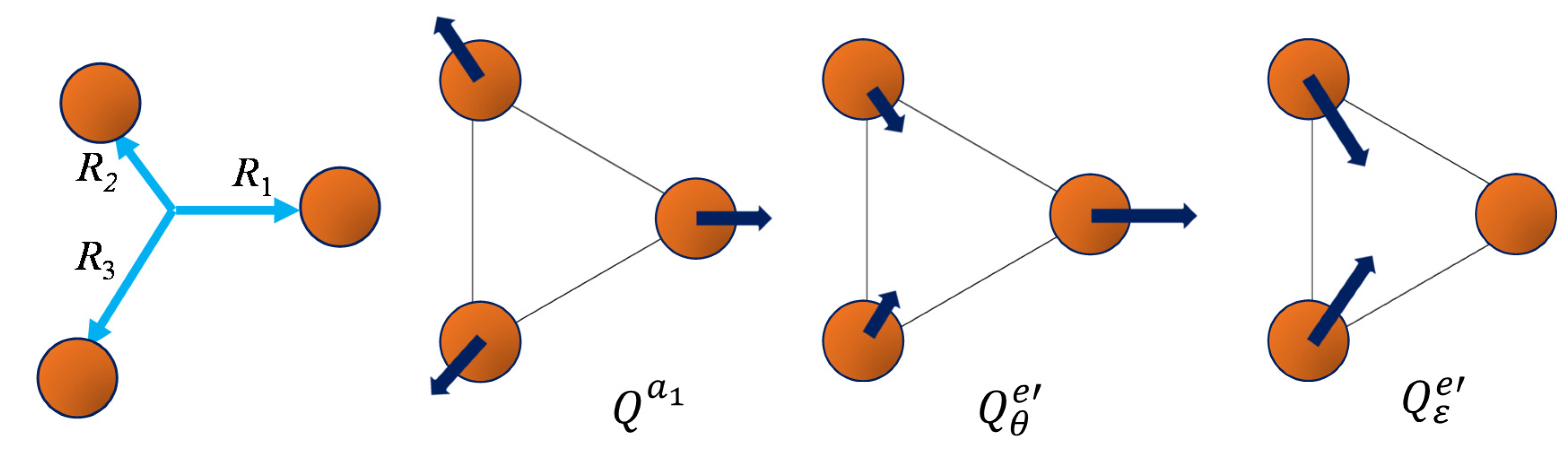
We conducted the calculations to generate the ab initio potential energy surfaces of the Jahn–Teller effect in the C₃H₃ system. In this view, we did a relaxed geometry scan, where the structure of the C₃ moiety is generated by tuning the distortion coordinates having the e′ symmetry, while the hydrogen atoms, i.e., the C-H bond lengths and CCH bond angles, were the subject of gradient refinement to optimized values.

The coordinates tuning the geometry of the triangle are chosen as symmetrized combinations of the edge lengths [47]. Here, we propose a different way, starting from the idea of defining a general triangle by three radii, R₁, R₂, and R₃, along axes fixed at mutual 120° angles. In spite of the constrained directions, the degrees of freedom are sufficient for defining any triangular configuration. In principle, even a negative R_i can be admitted, but such an extreme evolution is not needed in our problem since relatively small displacements from the equilateral reference are expected when $R_1=R_2=R_3=l_{CC}\left(D_{3h}\right)/\sqrt{3}$ as a function of the carbon–carbon bond-length in the system at the conical intersection. Then, we chose the symmetrized coordinates as a linear transformation over the above-defined radii:

$$Q^{a_1}=\frac{R_1}{\sqrt{3}}+\frac{R_2}{\sqrt{3}}+\frac{R_3}{\sqrt{3}},$$

(17a)

$$Q_{\theta }^{e^{\prime }}=\sqrt{\frac{2}{3}}{R}_1-\frac{R_2}{\sqrt{6}}-\frac{R_3}{\sqrt{3}},$$

(17b)

$$Q_{\epsilon }^{e^{\prime }}=\frac{R_2}{\sqrt{2}}-\frac{R_3}{\sqrt{2}}.$$

(17c)

Figure 6 illustrates the above-defined coordinates.

The total symmetric coordinate is not of direct interest in the discussed potential energy surface, being fixed at the geometry of the optimized conical intersection: $Q^{a_1}=l_{CC}\left(D_{3h}\right)=1.377 \mathrm{\AA }$. The coordinates generically labeled e in the introductory discussion are, more specifically, e′ in the case of the triangle. The components with the θ and ε subscripts in Equations (17b) and (17c) correspond to the ρ·cos(φ) and ρ·sin(φ) definitions, respectively, with the polar coordinates discussed in Section 3.1.

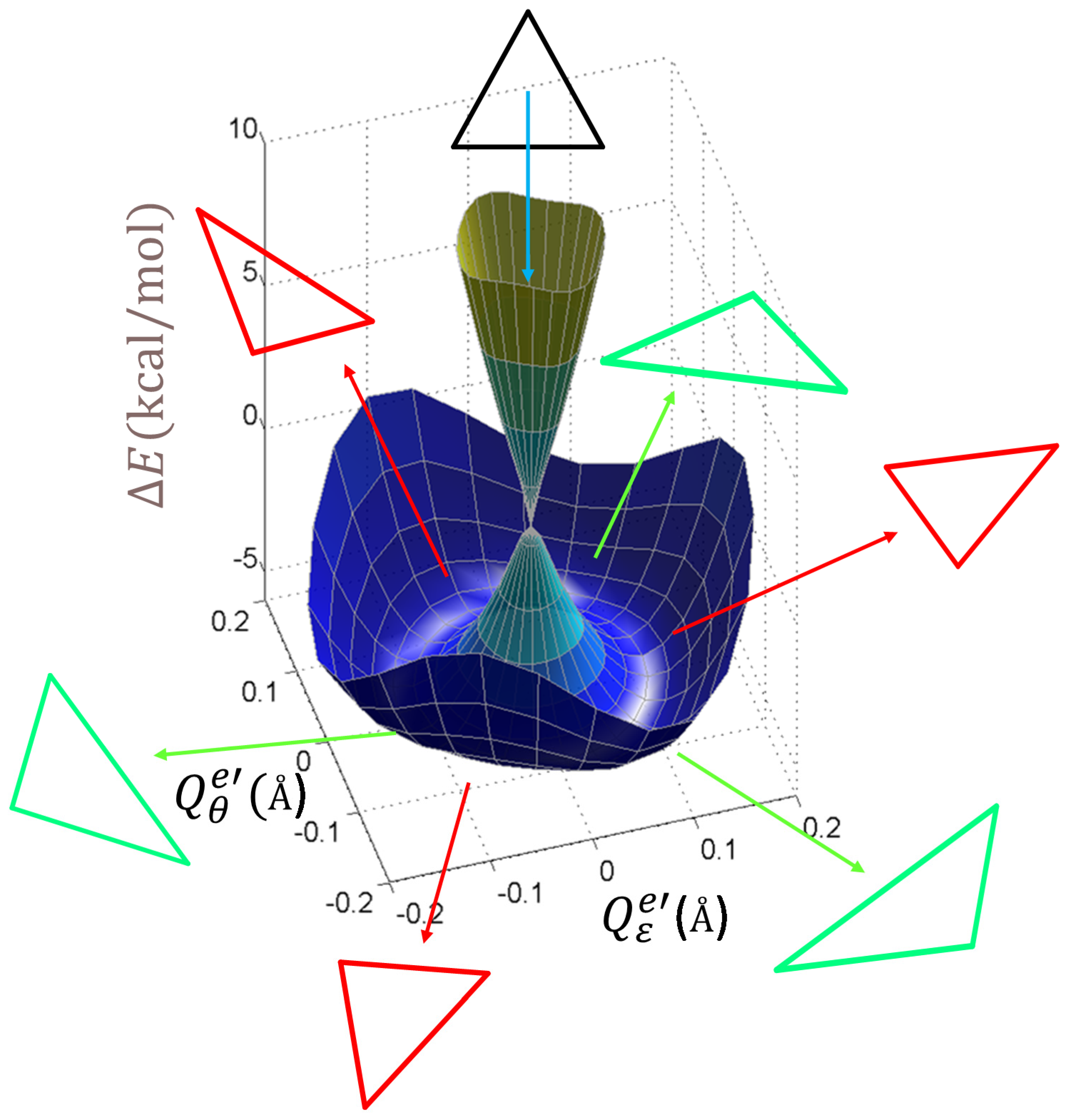
As a technical detail, we performed an ab initio scan on a grid in polar coordinates and backward converted these to the geometry of the carbon-based triangle. The radial points run between ρ = 0 and ρ = 0.2 Å, with a δρ = 0.02 Å step, the polar coordinate going around the circle with a δφ = 15° increment. The points collected for the lowest two CASSCF states are represented as surfaces in Figure 7. To distinguish it from the idealized model in Section 3.1, which, confined to first-order vibronic coupling terms, had a continuous circular minimum at the bottom of the e₋(ρ) surface, the realistic system is warped in a trigonal pattern, showing three minima and three saddle points in the quasi-circular valley. To account for this, the model should be updated with second-order vibronic coupling terms [2,3], namely the W parameter in the new eigenvalue equations:

$$e_{\pm }\left(\rho ,\phi \right)=\frac{1}{2}K{\rho }^2\pm \rho \sqrt{V^2+{\rho }^2{W}^2+2\rho \cdot V\cdot W\cdot \cos \left(3\phi \right)}.$$

(18)

This model acquires a dependence on the polar angle, the 3φ term in Equation (18) accounting for the three-fold symmetry implied by the C₃ axis of the molecule. The angular dependence modulates three minima and three maxima around the former circular trough of the minimum from the previous simplified level of the model (with W = 0). Since on the bottom of the valley the curvature with respect to the radial variable remains positive (corresponding to the minimum), the maxima with respect to the angular parameter (negative curvature) are actually saddle points. The absolute minima (the three equivalent positions at φ = 0 and ±120°) show a positive curvature (the second derivative of the above-defined eigenvalues) with respect to both the ρ and φ variables.

The computed points represented as surfaces in Figure 3 were reasonably fitted with Equation (18) by the following optimized parameters: K = 942.256 kcal·mol⁻¹Å⁻², V = 102.996 kcal·mol⁻¹Å⁻¹, and W = 34.349 kcal²·mol⁻²Å⁻⁴. The goodness of the fit can be measured by the linearity in the representation of the e_calc ab initio calculated energies vs. the e_fit values fitted by Equation (18). The least-square line e_fit = a·e_calc + b has a slope a = 1.001 and an R² = 0.994, close to the ideal unity values, while the intercept is small (b = 0.202 kcal/mol).

Given the novelty of the proposed geodesic analysis of the potential energy surfaces, we opted to proceed systematically from the simplest level of the prototypical E⊗e model, represented by Equations (1) and (2), while the real cases are better accounted for with the more complicated form (Equation (18)). As a compromise, we consider in the following the parameters fitted from the application to the cyclo-propenyl radical, dropping, however, the term corresponding the second-order coupling (i.e., imposing W = 0). 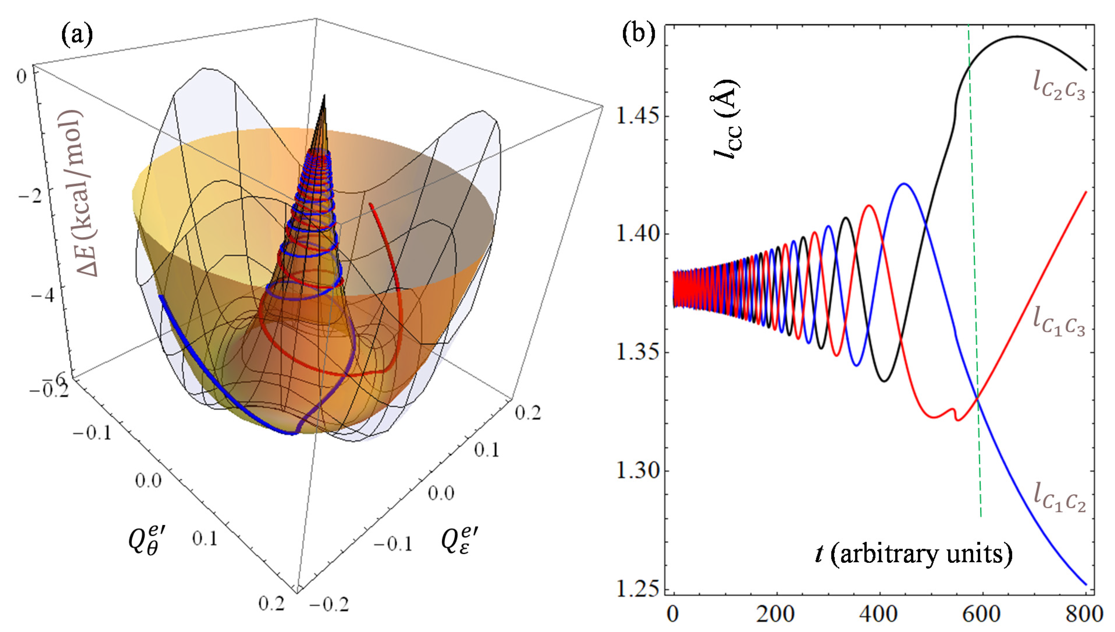This numeric experiment is presented in Figure 8.

Although the evolution parameter, t, can be intuitively thought of as time, we are considering it here in arbitrary units. In qualitative terms, the situation presented in Figure 8 is similar to panel (a) from Figure 1, while the aspect of the curve is sensibly different because of another interplay of parameters. In the Figure 8 case, we placed the initial point close to the conical intersection in order to simulate the evolution toward distortion, imposing a conventional value for the angular derivative. The larger the initial derivative, the steeper the descent on the conical part, with fewer coils until the minimum valley. A smaller initial derivative yields more loops, with successive spirals closer to each other. A mechanical interpretation of geodesics is the trajectory in the absence of a continuous source of acceleration [35]. Here, we do not consider this meaning, first of all because a mechanical trajectory is not literally accepted in a quantum model. At the same time, the geodesics appear as infinite curves, while the model itself is not conceivable over a very long range, being conceptually limited in the area containing the minimum of the lowest state and the conical intersection. On the other hand, the spiraling pattern of general geodesics can be tentatively put in connection with the intrinsic oscillatory nature of the problem, as the E⊗e model can be thought of as a sort of coupling between harmonic oscillators. The geodesic example from Figure 8 may suggest that, in the hypothetical case of instantaneous high symmetry, the system will probably evolve toward the distorted minimum in oscillatory progressions. The geodesics also continue after passing through the minimum valley. In a rough interpretation, this can be considered as being due to the impetus gained during the descent, but the continuation at a larger radius has no physical meaning. Therefore, there is a dissociation between the geometric geodesic and the mechanical or Born–Oppenheimer trajectory, which presumably encounters a barrier in terms of the reachable energy height. We let the connection between geodesics and the Born–Oppenheimer molecular dynamics trajectory be a matter of further investigations and debate. We hypothesize that a certain connection with the nodes of vibrational wave functions can be established, but we cannot exhaust here all the possible lemmas emerging from the problem.

4. Conclusions

We considered the phenomenological Hamiltonian of the prototypical E⊗e Jahn–Teller problem through the lens of geodesics analysis. We confined ourselves to the approximation of first-order vibronic coupling terms as analytic solutions of the geodesic curves on the E⊗e model surface are not obtainable. Then, we analyzed in qualitative respects possible types of geodesics on the basis of numerical solutions to the subsequent differential equations. We presented analytical forms of geodesics only for the region of the conical intersection, driven by the linear term of the vibronic model.

As a concrete simple example of the E⊗e Jahn–Teller effect, we considered the cyclo-propenyl molecular radical C₃H₃ undergoing spontaneous distortion from the conceivably higher geometry of the equilateral triangle. We performed a CASSCF-based complete mapping of the two potential surfaces originating from the E term in D_3h symmetry as a function of e-type distortion coordinates. The realistic surfaces show a trigonal warping fitted by the intervention of the second-order vibronic coupling parameter. Here, we did not explore the case of the second-order coupling in the geodesics analysis; however, we aim to devote further systematic attention to this class of problems and plan to extend the analysis to other prototypic Jahn–Teller and related effects.

We must admit that we have not clarified all the possible physical implications of the proposed characterization of potential energy surfaces by geodesic analysis, as we merely aimed to point out a new way and leave it open to debate and broader contributions. A rather obvious connection to the Born–Oppenheimer molecular dynamics could be stated, but we refrained explicitly from considering the evolution parameter as the time, in order to avoid entering immediately into the technical intricacies of this domain.

References

1. Jahn, H.A.; Teller, E. Stability of polyatomic molecules in degenerate electronic states-I—Orbital degeneracy. Proc. R. Soc. Lond. A 1937, 161, 220–235. [Google Scholar]
2. Bersuker, I.B. The Jahn–Teller Effect and Vibronic Interactions in Modern Chemistry; Plenum Press: New York, NY, USA, 1984. [Google Scholar]
3. Bersuker, I.B.; Polinger, V.Z. Vibronic Interactions in Molecules and Crystals; Springer: Berling, Germany, 1989. [Google Scholar]
4. Born, M.; Oppenheimer, R. Zur Quantentheorie der Molekeln. Ann. Physik 1927, 389, 457–484. [Google Scholar]
5. Jensen, F. Introduction to Computational Chemistry; Wiley: Chichester, UK, 2007. [Google Scholar]
6. Putz, M.V.; Cimpoesu, F.; Ferbinteanu, M. Structural Chemistry, Principles, Methods, and Case Studies; Springer: Cham, Switzerland, 2018. [Google Scholar]
7. Bersuker, I.B. Pseudo-Jahn–Teller effect: A two-state paradigm in formation, deformation, and transformation of molecular systems and solids. Chem. Rev. 2013, 113, 1351–1390. [Google Scholar] [CrossRef] [PubMed]
8. Martin, R.M. Electronic Structure: Basic Theory and Practical Methods; Cambridge University Press: Cambridge, UK, 2004. [Google Scholar]
9. Cotton, F.A. Chemical Applications of Group Theory, 3rd ed.; Wiley: New York, NY, USA, 1990. [Google Scholar]
10. Bunker, P.R.; Jensen, P. Fundamentals of Molecular Symmetry; CRC Press: Boca Raton, FL, USA, 2005. [Google Scholar]
11. Hoffmann, M.R.; Laidig, W.D.; Kim, K.S.; Fox, D.J.; Schaefer, H.F., III. Electronic symmetry breaking in polyatomic molecules. Multiconfiguration self-consistent field study of the cyclopropenyl radical C3H3. J. Chem. Phys. 1984, 80, 338–343. [Google Scholar] [CrossRef] [Green Version]
12. Glukhovtsev, M.N.; Laiter, S.; Pross, A. Thermochemical assessment of the aromatic and antiaromatic characters of the cyclopropenyl cation, cyclopropenyl anion, and cyclopropenyl radical: A high-level computational study. J. Phys. Chem. 1996, 100, 17801–17806. [Google Scholar] [CrossRef]
13. Moffitt, W.; Thorson, W. Vibronic states of octahedral complexes. Phys. Rev. 1957, 108, 1251–1255. [Google Scholar] [CrossRef]
14. Deeth, R.J.; Hitchman, M.A. Factors influencing Jahn–Teller distortions in six-coordinate copper (II) and low-spin nickel (II) complexes. Inorg. Chem. 1985, 25, 1225–1233. [Google Scholar] [CrossRef]
15. O’Brien, M.C.M. Dynamic Jahn–Teller effect in octahedrally Co-ordinated d9 ions. Proc. R. Soc. Lond. A 1964, 281, 323–339. [Google Scholar]
16. Lee, J.H.; Delaney, K.T.; Bousquet, E.; Spaldin, N.A.; Rabe, K.M. Strong coupling of Jahn–Teller distortion to oxygen-octahedron rotation and functional properties in epitaxially strained orthorhombic LaMnO3. Phys. Rev. B 2013, 88, 174426. [Google Scholar] [CrossRef] [Green Version]
17. Berry, M.V. Quantal phase factors accompanying adiabatic changes. Proc. Roy. Soc. Lond. A 1984, 392, 45–57. [Google Scholar]
18. Cimpoesu, F.; Ferbinteanu, M.; Humelnicu, I.; Mihai, A. The symmetry blueprints of the molecular edifices. Symmetry Cult. Sci. 2008, 19, 397–414. [Google Scholar]
19. Toader, A.M.; Buta, C.M.; Frecus, B.; Mischie, A.; Cimpoesu, F. Valence bond account of triangular polyaromatic hydrocarbons with spin: Combining ab initio and phenomenological approaches. J. Phys. Chem. C 2019, 123, 6869–6880. [Google Scholar] [CrossRef]
20. Buta, M.C.; Frecus, B.; Enache, M.; Humelnicu, I.; Toader, A.M.; Cimpoesu, F. Intra- and inter-molecular spin coupling in phenalenyl dimeric systems. J. Phys. Chem. A 2021, 125, 6893–6901. [Google Scholar] [CrossRef]
21. Toader, A.M.; Buta, M.C.; Mischie, A.; Putz, M.V.; Cimpoesu, F. The density functional theory account of interplaying long-range exchange and dispersion effects in supramolecular assemblies of aromatic hydrocarbons with spin. Molecules 2022, 27, 45. [Google Scholar] [CrossRef]
22. Toader, A.M.; Buta, M.C.; Maftei, D.; Putz, M.V.; Cimpoesu, F. Atoms in generalized orbital configurations: Towards atom-dedicated density functionals. Int. J. Mol. Sci. 2019, 20, 5943. [Google Scholar] [CrossRef] [Green Version]
23. Jianu, M.; Achimescu, S.; Daus, L.; Mihai, A.; Roman, O.A.; Tudor, D. Characterization of rectifying curves by their involutes and evolutes. Mathematics 2021, 9, 3077. [Google Scholar] [CrossRef]
24. Aydin, M.E.; Mihai, A. A note on surfaces in space forms with Pythagorean fundamental forms. Mathematics 2020, 8, 444. [Google Scholar] [CrossRef] [Green Version]
25. Aydin, M.E.; Mihai, A. Ruled surfaces generated by elliptic cylindrical curves in the isotropic space. Georgian Math. J. 2019, 26, 331–340. [Google Scholar] [CrossRef]
26. Wolfram, S. The Mathematica Book, 5th ed.; Wolfram-Media: Champaign, IL, USA, 2003. [Google Scholar]
27. Mathematica Software, Version 13.0; Wolfram Research Inc.: Champaign, IL, USA, 2014.
28. MATLAB, Version 6; The MathWorks Inc.: Natick, MA, USA, 2000.
29. Eaton, J.W.; Bateman, D.; Hauberg, S.; Wehbring, R. GNU Octave, Version 3.8.1; 2014. Available online: https://www.gnu.org/software/octave/ (accessed on 20 January 2022).
30. Schmidt, M.W.; Baldridge, K.K.; Boatz, J.A.; Elbert, S.T.; Gordon, M.S.; Jensen, J.H.; Koseki, S.; Matsunaga, N.; Nguyen, K.A.; Su, S.; et al. General atomic and molecular electronic structure system. J. Comput. Chem. 1993, 14, 1347–1363. [Google Scholar] [CrossRef]
31. Gordon, M.S.; Schmidt, M.W. Advances In electronic structure theory: GAMESS a decade later. In Theory and Applications of Computational Chemistry, the First Forty Years; Dykstra, C.E., Frenking, G., Kim, K.S., Scuseria, G.E., Eds.; Elsevier: Amsterdam, The Netherlands, 2005; Chapter 41; pp. 1167–1189. [Google Scholar]
32. Dunning, T.H. Gaussian basis sets for use in correlated molecular calculations. I. The atoms boron through neon and hydrogen. J. Chem. Phys. 1989, 90, 1007–1023. [Google Scholar] [CrossRef]
33. Hilderbrandt, R.L. Cartesian Coordinates of Molecular Models. J. Chem. Phys. 1969, 51, 1654–1659. [Google Scholar] [CrossRef]
34. Schaftenaar, G.; Noordik, J.H. Molden: A pre- and post-processing program for molecular and electronic structures. J. Comput.-Aided Mol. Design. 2000, 14, 123–134. [Google Scholar] [CrossRef]
35. do Carmo, M.P. Differential Geometry of Curves and Surfaces; Prentice-Hall: Hoboken, NJ, USA, 1976. [Google Scholar]
36. Applegate, B.E.; Barckholtz, T.A.; Miller, T.A. Explorations of conical intersections and their ramifications for chemistry through the Jahn—Teller effect. Chem. Soc. Revs. 2003, 32, 38–49. [Google Scholar] [CrossRef]
37. Domcke, W.; Yarkony, D.R.; Koppel, H. (Eds.) Conical Intersections: Electronic Structure, Dynamics and Spectroscopy; World Science: Singapore, 2004. [Google Scholar]
38. Lipschutz, M. Schaum’s Outline of Theory and Problems of Differential Geometry; McGraw-Hill Book Company: New York, NY, USA, 1969. [Google Scholar]
39. Mahapatra, S.; Köppel, G. Quantum mechanical study of optical emission spectra of Rydberg-excited H3 and its isotopomers. Phys. Rev. Lett. 1998, 81, 3116–3120. [Google Scholar] [CrossRef]
40. Mistrík, I.; Reichle, R.; Helm, H.; Müller, U. Predissociation of H3 Rydberg states. Phys. Rev. A 2001, 63, 042711. [Google Scholar] [CrossRef]
41. Oka, T. Interstellar H3+. Chem. Rev. 2013, 113, 8738–8761. [Google Scholar] [CrossRef]
42. Wheeler, S.E.; Robertson, K.A.; Allen, W.D.; Schaefer, H.F.; Bomble, Y.J.; Stanton, J.F. Thermochemistry of key soot formation intermediates: C3H3 isomers. J. Phys. Chem. A 2007, 111, 3819–3830. [Google Scholar] [CrossRef]
43. Cirelli, G.; Graf, F.; Günthard, H.H. ESR spectrum of the cyclopropenyl radical. Chem. Phys. Lett. 1974, 28, 494–496. [Google Scholar] [CrossRef]
44. Closs, G.L.; Redwine, O.D. Characterization of matrix- isolated cyclopropen-3-yl by EPR Spectroscopy. J. Am. Chem. Soc. 1986, 108, 506–507. [Google Scholar] [CrossRef]
45. Closs, G.L.; Evanochko, W.T.; Norris, J.R. Structure and dynamics of the trimethylcyclopropenyl radical as determined by electron and nuclear magnetic resonance. J. Am. Chem. Soc. 1982, 104, 350–352. [Google Scholar] [CrossRef]
46. Schreiner, K.; Ahrens, W.; Berndt, A. ESR proof of the antiaromaticity of a cyclopropenyl radical. Angew. Chem. Int. Ed. Engl. 1975, 14, 550–551. [Google Scholar] [CrossRef]
47. Davidson, E.R.; Borden, W.T. The potential surface for planar cyclopropenyl radical and anion. J. Chem. Phys. 1977, 67, 2191–2196. [Google Scholar] [CrossRef]
48. Poppinger, D.; Radom, L.; Vincent, M.A. On the Jahn-Teller distortion in the cyclopropenyl radical. Chem. Phys. 1977, 23, 437–442. [Google Scholar] [CrossRef]
49. Chipman, D.M.; Miller, K.E. Theoretical study of the cyclopropenyl radical. J. Am. Chem. Soc. 1984, 106, 6236–6242. [Google Scholar] [CrossRef]
50. Tachibana, A.; Asai, Y.; Ikeuchi, S.; Ishikawa, S.; Yamabe, T. Isomorphic electron orbitals for vibronic flexibility in a cyclopropenyl radical molecular device. Theoret. Chim. Acta 1990, 78, 1–9. [Google Scholar] [CrossRef]
51. Guo, M.; Wang, Z.; Wang, F. Stationary points on potential energy surface of cyclic C3H3 with coupled-cluster approaches and density functional theory. J. Phys. Chem. A 2021, 125, 4079–4088. [Google Scholar] [CrossRef]
52. Bartlett, R.J.; Musiał, M. Coupled-cluster theory in quantum chemistry. Rev. Mod. Phys. 2007, 79, 291–352. [Google Scholar] [CrossRef] [Green Version]
53. Knowles, P.J.; Werner, H.-J. An efficient second-order MCSCF method for long configuration expansions. Chem. Phys. Lett. 1985, 115, 259–267. [Google Scholar] [CrossRef]
54. Schmidt, M.W.; Gordon, M.S. The construction and interpretation of MCSCF wavefunctions. Annu. Rev. Phys. Chem. 1998, 49, 233–266. [Google Scholar] [CrossRef] [Green Version]
55. Kayi, H.; Garcia-Fernandez, P.; Bersuker, I.B.; Boggs, J.E. Deviations from Born-Oppenheimer Theory in Structural Chemistry: Jahn-Teller, Pseudo Jahn-Teller, and Hidden Pseudo Jahn-Teller Effects in C3H3 and C3H3. J. Phys. Chem. A 2013, 117, 8671–8679. [Google Scholar] [CrossRef]
Figure 1. Geodesics with the ρ ˙ P = 0 initial condition, qualitatively distinct as a function of the placement of the starting point ρP. The panels (ac) correspond to an initial point on the lower surface (ground-state), while (d) corresponds to the point on the higher solution (excited state). The situations (ac) for ρP < ρmin, ρP = ρmin, and ρP > ρmin, respectively, where ρmin is the radius of the circular trough defining the minimum of the ground surface. In the case of (d), the qualitative pattern is similar, irrespective of the position of the starting point. The initial point (ρP, φP = 0) occurs where the red and blue colors come into contact. The two halves of the geodesic, with different colors, result from the opposite signs of the non-null φ ˙ P 0 initial condition.
Symmetry 14 00436 g001
Figure 2. Geodesics with the φ ˙ P = 0 initial condition: (a) the starting point is placed on the lower energy surface; (b) the starting point is situated in the higher state. The two halves of the geodesic result from opposite signs of the non-null ρ ˙ P 0 initial condition.
Symmetry 14 00436 g002
Figure 3. Upper view (along the vertical axis) of general geodesics, illustrated for a distinct starting point P: (a) 0 < ρP < ρmin on the e(ρ) surface; (b) ρP = ρmin on the e(ρ) surface; (c) ρP > ρmin on the e(ρ) surface; (d) any ρP vs. ρmin’s relative placement on the e+(ρ) surface. The coloring of the curves discriminates qualitatively different initial conditions of the subsequent differential equations. The red curves represent the ρ ˙ P = 0 initial derivative, being just a different view of the geodesics represented in Figure 1 (the merged red and blue halves from Figure 1 being shown here all in red). The green and blue geodesics stand for, respectively, in the order of increasing absolute value of the | ρ ˙ P | radial velocity. The red, green, and blue curves start from the same point, their crossing in P being marked by a circle.
Symmetry 14 00436 g003
Figure 4. Different patterns for a geodesic on the cone. Left side: the case with the ρ ˙ P = 0 initial condition. Right side: a situation with ρ ˙ P > 0 . The red and blue halves starting from the initial point correspond to the φ ˙ P > 0 and φ ˙ P < 0 situations, respectively.
Symmetry 14 00436 g004
Figure 5. Optimized molecular geometries and qualitative π-type orbital schemes for the C3H3 radical in a high-symmetry structure (left side, D3h point group) and at a distorted stationary point (right side, C2v point group). The bond lengths marked on molecular geometries are all in Ångstrom units (Å).
Symmetry 14 00436 g005
Figure 6. Left-side snippet: convened system for defining the vertices of general triangles by the lengths of three radii fixed at mutual 120° angles. The following frames mark the displacements along the R 1 , R 2 , and R 3 vectors corresponding to the total symmetry at the a1 coordinate and the two degenerate elements of the e′ representation, respectively.
Symmetry 14 00436 g006
Figure 7. Computed relaxed potential energy surfaces emulating the Ee Jahn–Teller effect in the cyclo-propenyl radical C3H3. The triangles annotated on the extrema points at the bottom of the lowest surface qualitatively suggest the distortion trend. The green triangles with open angles correspond to the minima (their absolute geometry being realistically represented on the right side of Figure 5). The acute red triangles stand for saddle points around the circular trough. The geometry at the conical intersection is the equilateral triangle (realistically shown on the left side of Figure 5). The relative energy is given in kcal/mol, with the zero value fixed at the conical intersection. The distortion coordinates are presented in Ångstrom units.
Symmetry 14 00436 g007
Figure 8. Example of a geodesic on the model potential energy adapted from the parameters fitted for the cyclo-propenyl radical. (a) The surface represented by the mesh corresponds to the lowest eigenvalue from the model with the fitted K, V, and W parameters, the solid transparent surface results taking the fitted K and V parameters and imposing W = 0. The red and blue curves evolving on the solid surface correspond to the symmetrical branches of a geodesic starting at ρP = 0.05 Å and φP = 0 with the ρ ˙ P = 0 and φ ˙ P = 1.0   initial conditions. (b) The lengths of the edges in the C3 triangle along the geodesic sequence presented in the red line from the left-side panel as a function of the conventional evolution parameter t. The blue half of the geodesic has the same evolution if we permute the C1-C3 vs. C1-C2 bond length values. The atom labels are given in Figure 5. The vertical dashed line passes through the minimum of the surface. The small differences between the values of bond lengths at the minimum inferred from this graph vs. those from quantum optimization, described in Figure 5, come from the W = 0 approximation enforced in the actual case.
Symmetry 14 00436 g008
Publisher’s Note: MDPI stays neutral with regard to jurisdictional claims in published maps and institutional affiliations.