Quasi-Analytical Solution of Optimum and Maximum Depth of Transverse V-Groove for Drag Reduction at Different Reynolds Numbers

Abstract

Reducing the skin-friction drag of a vehicle is an important way to reduce carbon emissions. Previous studies have investigated the drag reduction mechanisms of transverse grooves. However, it is more practical to investigate which groove geometry is optimal at different inflow conditions for engineering. The purpose of this paper is to establish the physical model describing the relationship between the dimensionless depth ($H^{+}=H{u}_{\tau }/\upsilon$) of the transverse groove, the dimensionless inflow velocity ($U_{\infty }^{+}=U_{\infty }/u_{\tau }$), and the drag reduction rate ($\eta$) to quasi-analytically solve the optimal and maximum transverse groove depth according to the Reynolds numbers. Firstly, we use the LES with the dynamic subgrid model to investigate the drag reduction characteristics of transverse V-grooves with different depths (h = 0.05~0.9 mm) at different Reynolds numbers ($1.09\times {10}^4~5.44\times {10}^5$) and find that $H^{+}$ and $U_{\infty }^{+}$ affect the magnitude of slip velocity ($U_s^{+}$), thus driving the variation of the viscous drag reduction rate (${\eta }_{\nu }$) and the increased rate of pressure drag (${\eta }_p$). Moreover, the relationship between $U_s^{+}$, ${\eta }_{\nu }$, and ${\eta }_p$ is established based on the slip theory and the law of pressure distribution. Finally, the quasi-analytical solutions for the optimal and maximum depths are solved by adjusting $U_s^{+}$ to balance the cost (${\eta }_p$) and benefit (${\eta }_{\nu }$). This solution is in good agreement with the present numerical simulations and previous experimental results.

1. Introduction

In recent years, due to the increase in energy consumption and the strict requirements of fuel efficiency, the technologies of reducing carbon emissions associated with skin-friction drag reduction have drawn much attention [1]. For Lufthansa Cargo’s Boeing 777F freighters, reducing the skin-friction drag by 1% means annual savings of around 3700 tons of kerosene and just under 11,700 tons of ${\mathrm{CO}}_2$ emissions [2]. Compared with traditional drag reduction methods, bionic microstructures have a better potential for engineering applications because of their remarkable drag reduction properties and good applicability [3,4,5]. Previous studies have shown that there are two types of microstructure, one is the riblets imitating shark shin [6,7] and the other is the transverse grooves imitating dolphin skin [8,9,10,11], which are parallel and perpendicular to the flow direction, respectively. It has been reported that longitudinal riblets are capable of delivering a reduction of surface friction drag around 10% [12]. The drag reduction mechanism of longitudinal riblets is attributed to the damping of crossflow fluctuations or the uplift of turbulent streamwise vortices above the riblet valley [13,14,15].

The better drag reduction properties of transverse grooves have been proved by the latest research. Lee et al. [16] observed that the maximum measured drag reduction of 40% was achieved by a nanoporous transverse grooved plate. Liu et al. [17] used large eddy simulation (LES) technology to analyze entropy generation in the flow over a transverse grooved plate. The results showed that the total entropy generation in the near-wall region decreased by approximately 25%. Wang et al. [18] reported that an 18.76% net drag reduction was achieved by transverse grooves. These studies indicate that transverse grooves exhibit more significant potential for engineering applications than streamwise riblets.

At present, most studies focus on the drag reduction mechanisms of transverse grooves. Some studies suggested that the vortices formed within the grooves weaken the turbulence structure in the boundary layer near the wall [19,20]. The more popular perspective indicated that the vortices within the transverse grooves change the sliding friction into rolling friction at the solid–liquid interface, which is also named the “micro air-bearing phenomenon” [21,22,23,24,25]. Several studies focused on the Cassie–Baxter state to reduce the solid–liquid contact area and create a superhydrophobic effect over the transverse grooves [26,27,28]. The studies of Seo et al. [29], Lang et al. [30], and Mariotti et al. [31] showed that the vortices formed in the transverse grooves increase the momentum in the boundary layer near the wall, thus effectively controlling the flow separation.

All the above studies are of great significance to qualitatively explain the drag reduction mechanism of the transverse groove. However, it is of more practical interest to understand which groove geometry is optimal at different inflow conditions for engineering. To the best of the authors’ knowledge, compared with a large number of studies in the context of streamwise riblets, less is known regarding the parameter studies on transverse grooves. The drag reduction characteristics of transverse grooves are mainly determined by the shape, AR (ratio of groove width to depth), and depth. Cui et al. [22] conducted a numerical simulation on the pressure drop in microchannel flow over different transverse-grooved surfaces and found that the drag-reduction rate of V-shaped transverse grooves is better than that of rectangular transverse grooves. The experimental results of Liu et al. [32] demonstrated that the drag reduction performance was best when the AR is 2 at a Reynolds number of 50,000. The purpose of this paper is to establish the physical model describing the relationship between the dimensionless depth ($H^{+}=H{u}_{\tau }/\upsilon$) of the transverse groove, the dimensionless inflow velocity ($U_{\infty }^{+}=U_{\infty }/u_{\tau }$), and the drag reduction rate ($\eta$), so as to quasi-analytically solve the optimal and maximum transverse groove depth according to the different Reynolds numbers. The optimum depth of the transverse groove corresponds to the maximum drag reduction rate, and the maximum depth corresponds to the drag reduction rate of zero, which is the limit for the allowable machining error for engineering applications.

This paper is organized as follows. First, the numerical methodology is formulated in Section 2. Secondly, the drag reduction characteristics of transverse V-grooves with different depths at different Reynolds numbers are investigated by LES in Section 3. Then, in Section 4, the theoretical model for the optimal and maximum depth of the transverse groove is established. Based on this model, the quasi-analytical solution of the groove depth has been solved and several grooved plates with different groove depths have been designed to verify the drag reduction characteristics in Section 5. Finally, the conclusions are presented in Section 6.

2. Numerical Methodology

2.1. Solving Methods

The large eddy simulation (LES) method is used in the commercial software FLUENT 18.0 to obtain the induced drag reduction and flow characteristics [33,34]. A dynamic subgrid-scale (SGS) is chosen to model the unresolved small flow field scale motions [35,36]. The discretized continuity equation is solved using the Rhie and Chow method [37] to compute the mass flux at each face. The diffusion terms and the advection terms in the discretized momentum equations are solved using a second-order-accurate central-differencing discretization scheme and a second-order upwind scheme, respectively. Moreover, a second-order implicit time-stepping approach is used for temporal discretization. Thus, the space and time resolution of the numerical method is of second-order accuracy. For the pressure–velocity coupling, SIMPLE (Semi-Implicit method for pressure linked equations) is used to enforce the mass conservation and obtain the pressure fields. For the evaluation of gradients and derivatives, the least-squares cell-based gradient method is employed. The dimensionless physical timestep $\Delta tU/H\approx 0.02$ [38] is used, where U denotes the uniform velocity at the inlet and H represents the depth of grooves. The dimensionless time of statistical averaging is above $TU/H\approx 400$ [34] to obtain the time-averaged results.

2.2. Computational Domain and Boundary Conditions

The 3D computational domain and the boundary conditions are shown schematically in Figure 1 and

Table 1. Size of the computational domain and the corresponding number of grid nodes.

		Dimensionless Parameters	Nodes
$L_x^{+}$		667 + 83 + 83	100 + 1200 + 25
$L_y^{+}$		103	50
$L_z^{+}$		103	25
$∆x^{+}$	Groove	0.05	1200
	Other	<10	100 + 25
$∆y^{+}$		0.02~10	50

. The height and spanwise length of the computational domain are 25 mm ($L_y^{+}=L_z^{+}=103$) [34], which covers at least the thickness of the boundary layer under all the flow conditions. The total length of the computational domain is 200 mm ($L_x^{+}=833$). A smooth wall with a length of 160 mm is placed upstream of a grooved wall for the development of turbulence from laminar flow. Another smooth wall with a length of 20 mm is located downstream of the grooved wall to prevent the propagations of pressure perturbations at the outlet. The simulated grooved wall is about 20 mm long, consisting of different symmetric V-grooves profiles—whose AR is 2 (aspect ratios, S/H, where S represents the width of an individual groove) and depths are 0.05~0.9 mm (a baseline plate without grooves is also simulated in the same position). Reynolds numbers range from $1.09\times {10}^4$ to $5.44\times {10}^5$, which is based on the length of the flat wall placed upstream of a grooved wall (160 mm), the freestream velocity, and the viscosity of the fluid. At all the solid walls, the no-slip condition is specified. At the inlet of the computational domain, an ideal gas flows with uniform velocity and a freestream turbulence intensity of 1%, and the pressure condition is set at the outlet.

In order to verify that the normal height ($L_y^{+}$) and spanwise length ($L_z^{+}$) of the computational domain meet the requirements of LES, two normal heights ($L_y^{+}=$ 103 and 123.6) and two spanwise lengths ($L_z^{+}=$ 103 and 123.6) are chosen to investigate the effect on outcomes.

Table 2. Domain independence test (h = 0.1 mm, Re = $1.09\times {10}^4$ ).

${\mathit{L}}_{\mathit{x}}^{+}$	${\mathit{L}}_{\mathit{z}}^{+}$	Drag (N)
103	103	0.00272
	123.6	0.00273
123.6	103	0.00273
	123.6	0.00276

shows the simulation results of the total drag of the grooved plate. The drag hardly changes when the normal height and the spanwise length are greater than 103, which means that the results conducted with $L_x^{+}$ = 103 and $L_z^{+}$ = 103 in the present are adequate for the requirements of LES.

2.3. Grid Independence Study

The structured mesh is generated by commercial software, ICEM, as shown in Figure 2. The grid resolution and the number of grid nodes are shown in Table 1. The grids are clustered near the wall surface and the normal distance from the wall surface to the nearest grid points $Y^{+}$ is 0.04. The maximum normal grid resolution $∆y_{max}^{+}$ is less than 10. The streamwise grid resolution $∆x^{+}$ is 0.07 within the grooves, and $∆x_{max}^{+}$ is less than 10 in other streamwise positions. The spanwise grid resolution $∆z^{+}$ is 4.1 [34].

In order to verify that the grid resolution meets the requirements of the large eddy simulation, two streamwise grid resolutions within the groove $∆x^{+}$ (0.07 and 0.32) and two spanwise grid resolutions $∆z^{+}$ (4.1 and 10) are chosen to investigate the effect on the outcomes.

Table 3. Verification of grid resolution (h = 0.1 mm, Re = $1.09\times {10}^4$ ).

$∆{\mathit{x}}^{+} \left(\mathbf{Groove}\right)$	$∆{\mathit{z}}^{+}$	Drag (N)		Streamline
0.07	4.1	0.00274	$\to$
	10	0.00273
0.32	4.1	0.00273
	10	0.00275	$\to$

shows the simulation results for the drag of the grooved plate and the streamline inside the groove. The resistances of a grooved plate hardly change when $∆x^{+}=0.07$ (groove) and $∆z^{+}=4.1$, which are selected for deriving all the other results.

Figure 3 shows the relative error of the total resistance of a grooved plate (with symmetric V-grooves whose AR is 2) compared with that of a smooth plate (based on the total drag in the case of 2,403,465 grids) at five different grid-refinement levels. The resistances of a grooved plate and the baseline plate no longer change when the number of grid cells is greater than 1,603,491, and the relative difference is 0.0465%, which is used as the grid resolution in deriving all the other results.

2.4. Experimental Validation

In order to check the accuracy of the obtained numerical results, the results of the numerical simulation are compared with the relevant experimental data reported previously. The numerical results of velocity profiles over the grooved plates with a groove depth of 1.62 mm and groove width of 3.57 mm are compared with the experimental results obtained by Ahmadi-Baloutaki et al. [39] in Figure 4a,b (the Reynolds number based on the length of the grooved plate is $1.85\times {10}^5$, and the turbulence intensity is 0.4% and 4.4%, respectively). The simulated velocity profiles agree well with the previously published experimental results, suggesting that the present numerical approach has sufficient accuracy for predicting the drag reduction of transverse grooves (the relative error is found to be less than 3%). Moreover, Figure 4c,d show the experimental results [40] and numerical results of the velocity vector over the grooved plate, respectively. It is apparent that the simulation results show good predictions of the location and structure of the vortex formed within the groove, which indicates that the CFD method can accurately simulate the flow details over the grooved plate.

3. Characteristics of Drag Reduction Induced by Transverse V-Grooves with Different Depths at Different Reynolds Numbers

Before establishing the prediction model of the optimal and maximum depth, it is necessary to analyze the key physical factors affecting the drag reduction characteristics. In this section, the amounts of drag reduction induced by grooves with different depths at different Reynolds numbers are computed and the mechanisms of drag reduction are analyzed.

Figure 5 illustrates the variation in drag-reduction rate with depth at different Reynolds numbers. The drag-reduction rate is defined as,

$$\eta =\frac{F_G-F_R}{F_R}$$

(1)

in which $F_G$ and $F_R$ represent the resistance of the grooved plate and the baseline plate, respectively. The results show that the drag-reduction rate induced by the grooved plate first increases and then decreases with the increase of depth. At each Reynolds number, there is an optimal groove depth for maximum drag reduction and a maximum groove depth corresponding to the zero-drag reduction rate, which is qualitatively consistent with the results of the previous study in the context of streamwise riblets [12]. Interestingly, the optimal and maximum depth decrease with the increase in Reynolds number, as shown in

Table 4. Drag reduction rate of transverse grooves with different depths at different Reynolds numbers.

Re\h(mm)	0.05	0.1	0.15	0.25	0.3	0.35	0.4	0.45	0.5	0.6	0.65	0.7	0.8	0.9
	−1.4%	−1.7%	−2.1%	−2.5%	−2.6%	−2.8%	−3.3%	−4.0%	−4.6%
	−4.2%	−4.8%	−5.2%	−5.6%	−5.8%	−6.0%	−6.4%	−7.0%	−7.9%
	−5.0%	−5.5%	−6.1%	−6.8%	−7.1%	−7.3%	−7.6%	−8.2%	−8.8%
	−5.9%	−6.2%	−6.8%	−7.7%	−8.2%	−8.5%	−8.7%	−9.3%	−10.1%	−8.7%	−7.4%	−6.1%	−3.0%	0.3%
	−6.7%	−7.2%	−7.9%	−8.8%	−9.4%	−9.8%	−10.2%	−10.7%	−9.4%	−6.3%	−4.7%	−3.1%	0.7%
	−7.3%	−8.1%	−9.0%	−9.8%	−10.2%	−11.0%	−11.7%	−12.0%	−8.4%	−3.6%	−1.5%	1.5%
	−8.1%	−9.2%	−9.9%	−10.5%	−11.3%	−11.9%	−12.4%	−10.6%	−6.7%	−2.1%	0.5%
	−9.2%	−9.6%	−10.4%	−11.4%	−12.6%	−12.9%	−10.4%	−5.4%	−2.4%	0.8%
	−9.8%	−10.5%	−10.9%	−12.2%	−13.2%	−12.7%	−9.8%	−4.2%	0.2%
	−9.9%	−10.9%	−11.8%	−13.3%	−14.4%	−11.5%	−6.8%	−2.3%	1.0%
	−11.0%	−12.0%	−12.8%	−14.4%	−14.1%	−10.2%	−5.4%	0.2%				Optimal depth
	−10.4%	−11.0%	−12.0%	−12.3%	−9.2%	−6.2%	−3.3%	1.2%				Maximum depth
	−9.9%	−10.1%	−10.2%	−9.6%	−8.7%	0.4%
	−8.1%	−7.1%	−5.9%	−4.8%	−1.5%

. It is worth noting that because the groove depth in the simulation cases is discrete, the optimal groove depth chosen from Table 4 actually corresponds to the ‘near-maximum’ drag reduction rate, and the maximum depth actually corresponds to the ’near-zero’ drag reduction rate.

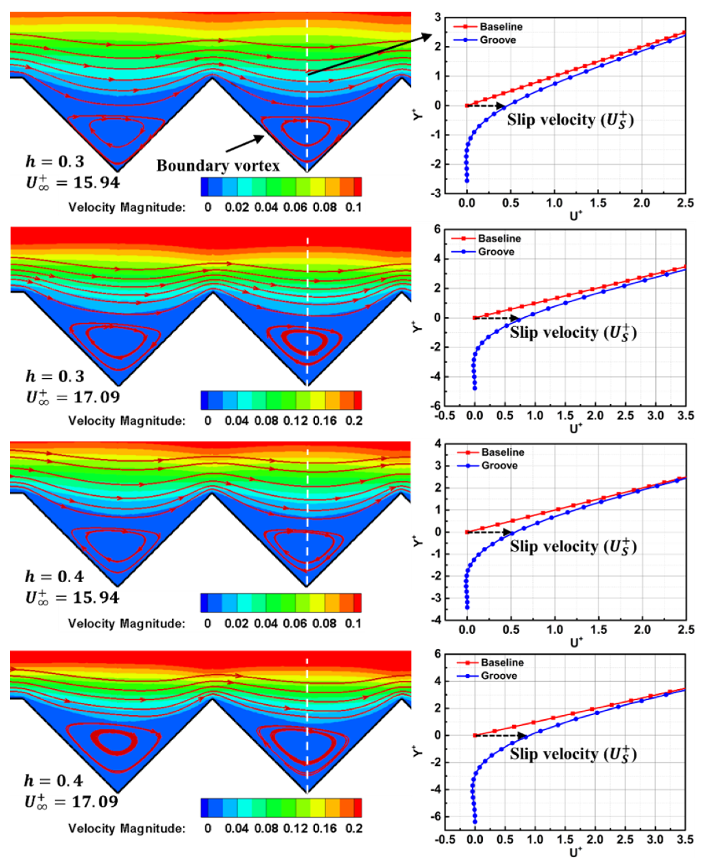
Figure 6 and Figure 7 show the flow details at different depths (h = 0.3 mm and h = 0.4 mm) and Reynolds numbers (to facilitate model building in the next section, we convert the Reynolds number into the dimensionless velocity, $U_{\infty }^{+}$, according to Equation (2) [41]) to analyze the physical mechanism driving the variation in total drag.

$$U_{\infty }^{+}=\frac{U_{\infty }}{u_{\tau }}=\frac{1}{\sqrt{0.029R{e}^{-0.2}}}$$

(2)

here, $u_{\tau }$ represents the local friction velocity.

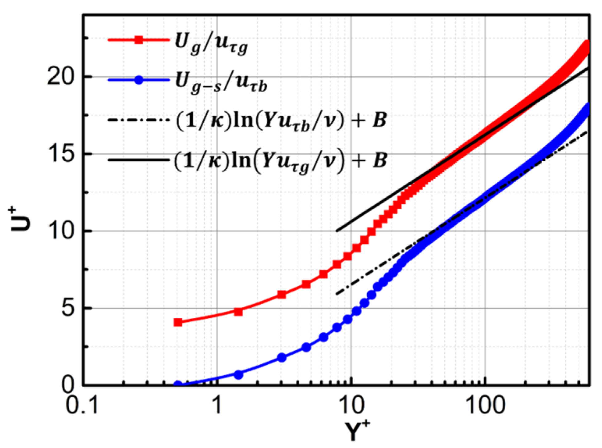
The streamline patterns and velocity that contour over the grooved plate are shown in Figure 6. Some vortices formed in the grooves can be distinctly observed as perpendicular to the flow direction. These boundary vortices act as “air bearings”, which separate the boundary layer from the solid wall, resulting in fluid sliding over the grooved plate. In order to measure the sliding degree, the dimensionless velocity profiles ($Y^{+}=y{u}_{\tau }/\nu$, and $U^{+}=U/u_{\tau }$) at the centerline of the grooved plate and the baseline plate at the corresponding position are compared (Figure 6, right). The results show that the velocity gradient over the grooved plate is less than that on the baseline plate, and an induced slip velocity ($U_s^{+}$) on the horizontal line can be selected as the quantitative parameter to describe the slip phenomenon. Moreover, the comparison results of the different numerical cases indicate that the slip velocity is affected by the groove depth (h) and inflow velocity ($U_{\infty }^{+}$).

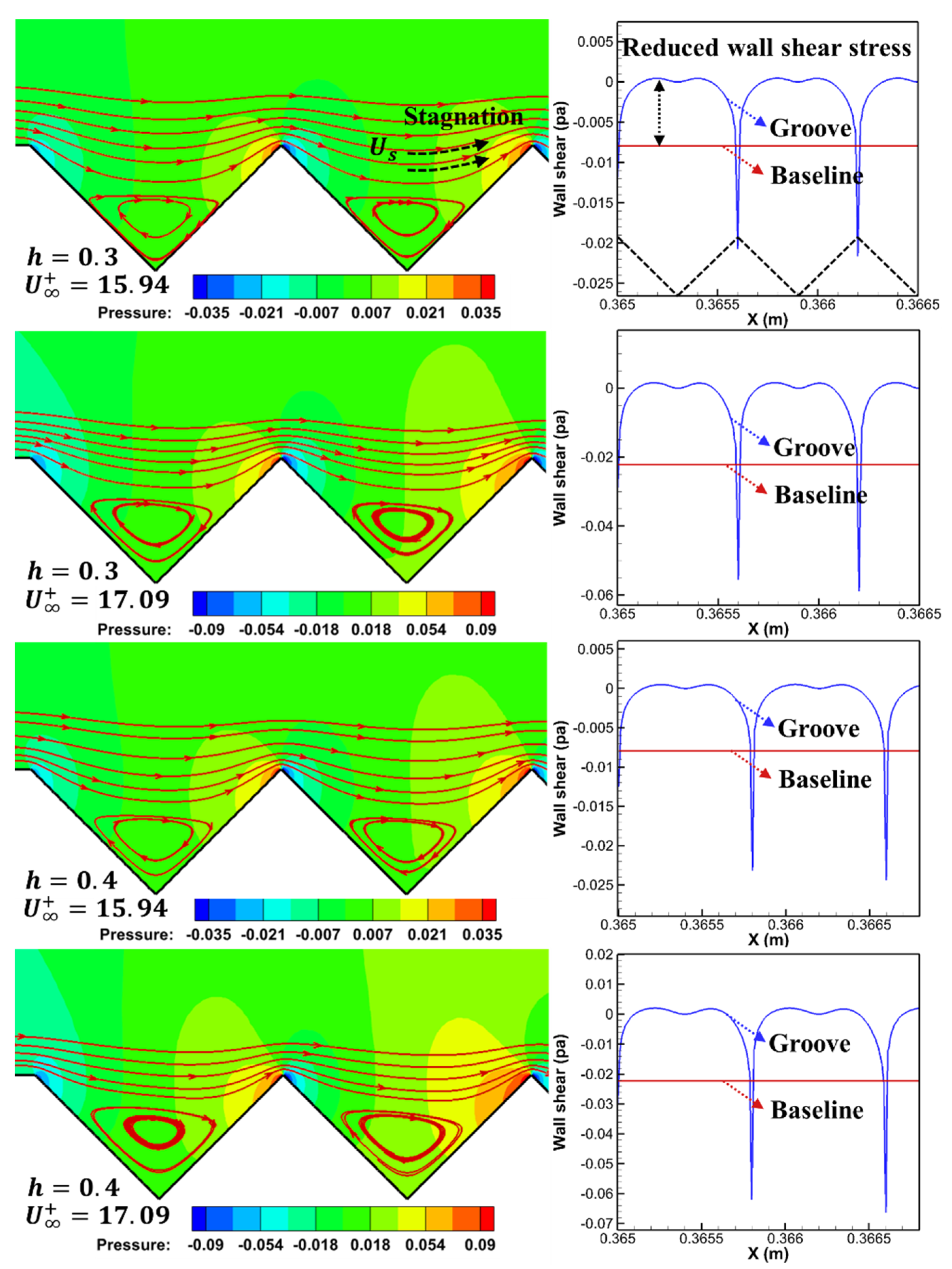
The wall shear distribution and pressure contour shown in Figure 7 further illustrate that the magnitude of slip velocities drives the variation in the total viscous drag and pressure drag. On the one hand, these slip velocities reduce the velocity gradient over the groove plate, thus reducing the total viscous resistance. This point is further proved by the shear stress distribution diagram, which shows that the shear stress of the grooved wall is significantly less than that of the baseline plate. By comparing the numerical cases of grooved plates with the same depth at different inflow velocities, it can be seen that the larger the slip velocity, the smaller the velocity gradient. As well, the corresponding shear stress decreases the most, so the total viscous resistance decreases the most in turn. On the other hand, the “slip fluids” induced by the vortices separate on the leeward side of the groove and stagnation occurs on the windward side, resulting in additional pressure drag compared to the baseline plate—which increases the total resistance of the grooved plate. The larger the slip velocity, the greater the stagnation pressure on the windward side, resulting in greater additional pressure drag. In summary, the grooved plate reduces the viscous drag (benefits) and increases the pressure drag (costs), and the optimal drag reduction is the result of balancing the benefits and costs.

From the above analysis, the total drag of the grooved plate consists of the viscous drag ($F_{GV}$) and pressure drag ($F_{GP}$), which are expressed by Equations (3) and (4), respectively. 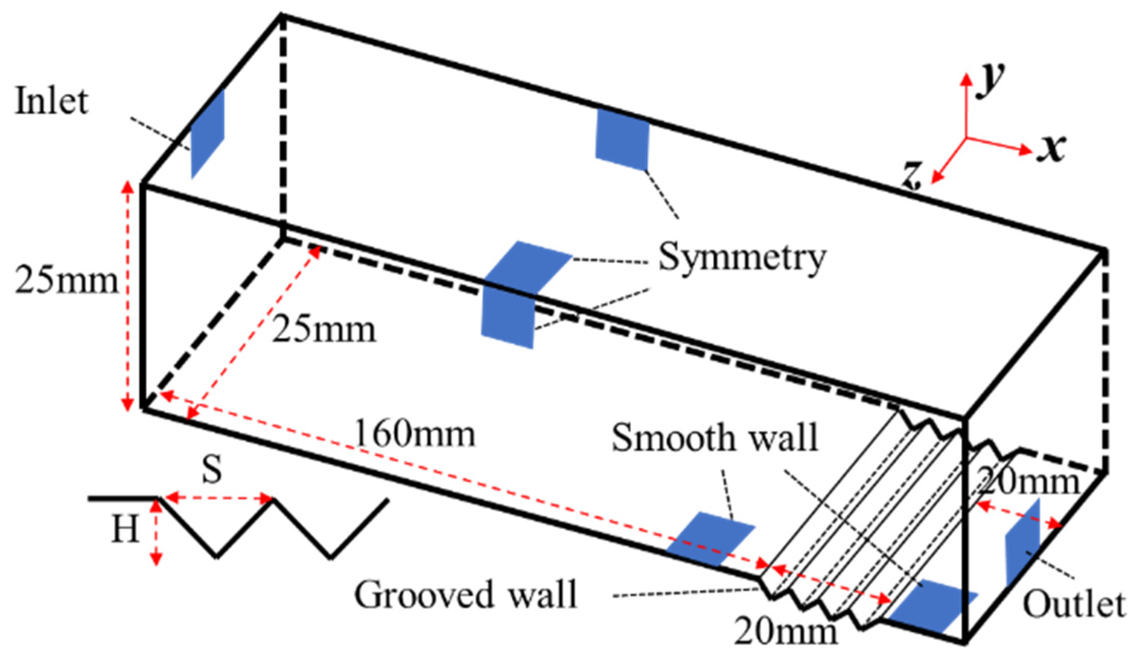$F_{GV}$ and $F_{GP}$ are determined by calculating the corresponding local stress—namely, shear ($\overline{\mathit{\tau }}$) and pressure (p) at the wall—and integrating the projected stress in the drag direction (${\overline{\mathit{e}}}_{\mathit{x}}$, that is the unit vectors in the x direction shown in Figure 1 along the wetted wall ($l_s$).

$$F_{GV}={{\displaystyle \int }}_0^{l_s}\overline{\mathit{\tau }}·{\overline{\mathit{e}}}_{\mathit{x}}dl$$

(3)

$$F_{GP}={{\displaystyle \int }}_0^{l_s}\left(p-p_{\infty }\right)\overline{\mathit{n}}·{\overline{\mathit{e}}}_{\mathit{x}}dl$$

(4)

here, $p_{\infty }$ represents the ambient pressure, l is the unit area along the groove wall, and $\overline{\mathit{n}}$ denotes the normal vector to the wall. Therefore, Equation (1) is transformed into Equation (5):

$$\eta =\frac{F_{GV}-F_R}{F_R}+\frac{F_{GP}}{F_R}={\eta }_{\nu }+{\eta }_p$$

(5)

here, ${\eta }_{\nu }=\left(F_{GV}-F_R\right)/F_R$ denotes the reduction rate for viscous drag, and “${\eta }_p=F_{GP}/F_R$” denotes the increased rate of pressure drag.

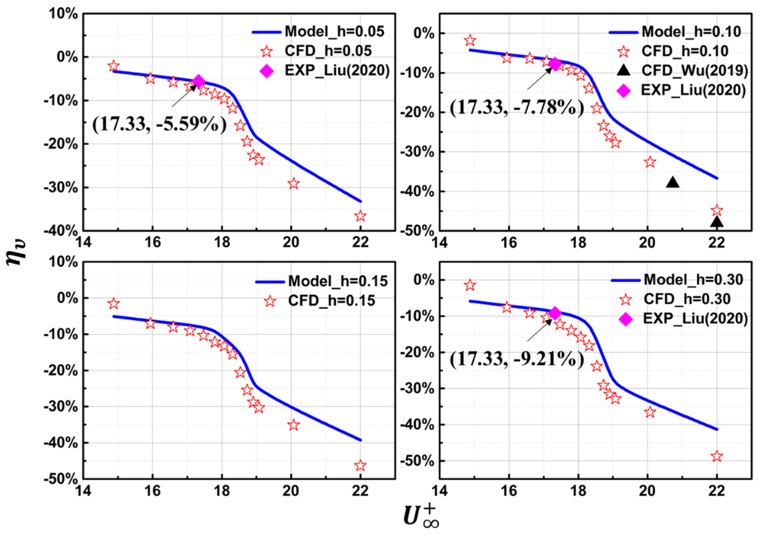
Figure 8 shows the variation of ${\eta }_{\nu }$ and ${\eta }_p$ with $U_s$, $u_t$, and $U_s^{+}$ (in order to compare the model results with the experimental results in the following sections, four different grooves with h of 0.05, 0.1, 0.15, and 0.3 mm are used for analysis). It can be seen that the absolute values of ${\eta }_{\nu }$ and ${\eta }_p$ increase with the increase of $U_s^{+}$ ($U_s^{+}=U_s/u_t$, where $u_t=\sqrt{{\tau }_{\omega }/\rho }$ is only a unit commonly used for dimensionless values. Therefore, there is no physical relationship between $u_t$ and the drag reduction rate), which further indicates that the slip velocity drives the variation in the total viscous drag and pressure drag. In conclusion, the essence of balancing the benefit (${\eta }_{\nu }$) and cost (${\eta }_p$) to obtain the optimal drag reduction is how to obtain the optimal slip velocity by matching the depth of the groove and the inflow velocity.

Based on the above analysis, we propose a model to match the relationship between inflow velocity ($U_{\infty }^{+}$) and groove depth (h) by determining the optimal slip velocity ($U_s^{+}$). The establishment process of this model is shown in Figure 9.

• Step 1. Construct the relationship between inflow velocity ($U_{\infty }^{+}$), depth ($H^{+}=h{u}_{\tau }/\nu$), and slip velocity ($U_s^{+}$).
• Step 2. Construct the physical relation between slip velocity ($U_s^{+}$) and viscous drag-reduction rate (${\eta }_{\nu }$).
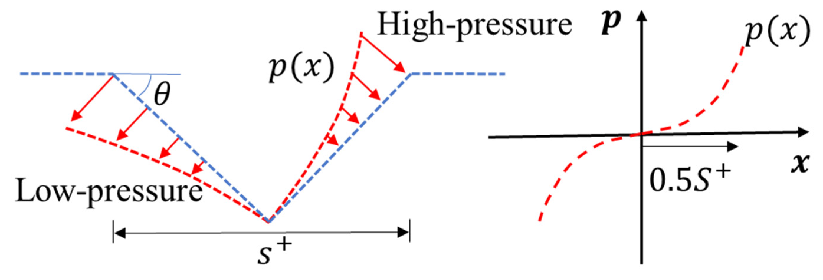
• Step 3. Construct the physical relation between slip velocity ($U_s^{+}$) and pressure drag-increase rate (${\eta }_p$).
• Step 4. Balance ${\eta }_{\nu }$ and ${\eta }_p$ to design the groove depth ($H^{+}$) in different inflow velocities ($U_{\infty }^{+}$).

4. Construction the Theoretical Model Describing the Relationship between the Dimensionless Depth (${\mathit{H}}^{\mathbf{+}}$), the Dimensionless Inflow Velocity (${\mathit{U}}_{\mathbf{\infty }}^{\mathbf{+}}$), and Drag Reduction Rate ($\mathit{\eta }$)

4.1. The Relationship between Slip Velocity ($U_s^{+}$), Depth ($H^{+}$), and Inflow Velocity ($U_{\infty }^{+}$)

The streamline patterns shown in Figure 7 reveal that the boundary vortices are not full inside the grooves. Therefore, we assume that the distances from the vortex center to the groove bottom and the slip surface are $Kh$ and $L_s$ (slip length, $L_s=\left(1-K\right)h$), respectively—as shown in Figure 10. Since the slip surface shown in Figure 10 (i.e., the position of the baseline plate) is at the viscous bottom layer, the total viscous stress can be expressed as

$${\tau |}_{slip}=\mu \frac{\partial u}{\partial y}={\tau }_{\omega }$$

(6)

Over the grooved plate, the velocity at the vortex core and the slip surface increases from 0 to $U_s$, and both $U_s$ and $L_s$ are small quantities, so the velocity gradient of U in the Y direction at the midpoint of the slip surface can be approximated as

$$\frac{\partial u}{\partial y}=\frac{{\tau }_{\omega }}{\mu }\approx \frac{U_s}{L_s}$$

(7)

in which ${\tau }_{\omega }=\rho {\left(u_{\tau }\right)}^2$, then Equation (7) can be transformed into Equation (8).

$$\frac{U_s}{u_{\tau }}=\frac{\rho u_{\tau }{L}_s}{\mu }$$

(8)

therefore, substituting “$L_s=\left(1-K\right)h$” into Equation (8) yields the relation between the dimensionless slip velocity and dimensionless depth, which is described as

$$U_s^{+}=\left(1-K\right)H^{+}$$

(9)

here, $U_s^{+}$ is equal to $U_s/u_{\tau }$, $H^{+}$ is equal to $\rho u_{\tau }h/\mu$, and K represents the fullness of the vortex within the groove, which varies with different inflow velocities and groove depths, as shown in the streamline patterns of Figure 11.

To quantitatively estimate the variation of K, we use the Boltzmann function to fit the data points (see Figure 12), which can be expressed as Equation (10). The resulting fits are accurate to better than 2% at a 95% confidence interval.

$$K=A_2+\left(\frac{A_1-A_2}{1+e^{\left(\left(U_{\infty }^{+}-U_0\right)/du\right)}}\right)$$

(10)

where $A_1$, $A_2$, $u_0$, and $du$ are the control parameters of the Boltzmann function, which can be described by Equation (11) (h is in millimeters).

$$\{\begin{array}{c}{A}_1=0.45809-0.32244h+0.79245h^2\\ A_2=0.74836+0.44569h-1.12162h^2\\ U_0=18.5287-9.83878h+6.70225h^2\\ du=0.33396+4.79502h-10.6357h^2\end{array}$$

(11)

therefore, substituting Equations (10) and (11) into Equation (9) yields Equation (12), which can predict the slip velocity over the groove plate with depth $H^{+}$ at the inflow velocity $U_{\infty }^{+}$.

$$U_s^{+}=f_1\left(H^{+},U_{\infty }^{+}\right)$$

(12)

Figure 13 compares the CFD data with the results of Equation (12). The results show that the prediction value of Equation (12) are qualitatively in agreement with the numerical simulations. In detail, when $h\le 0.1$, the prediction accuracy decreases with the increase of $U_{\infty }^{+}$, so Equation (12) is more adequate for the $14.88<U_{\infty }^{+}<18.53$. However, when $h>0.1$, Equation (12) has a greater prediction accuracy when the dimensionless inflow velocity is between $14.9$ and $22$.

4.2. The Relationship between Slip Velocity ($U_s^{+}$) and Viscous Drag-Reduction Rate (${\eta }_{\nu }$)

Fukagata and Kasagi [42] proposed a theoretical prediction model for the drag reduction rate achieved by superhydrophobic surfaces in a turbulent channel flow. By comparing the bulk mean velocity of the baseline plate and the hydrophobic surface, they successfully established the relationship between the streamwise and spanwise slip length and the drag reduction rate. Different from their work, our work aims to establish the relationship between slip velocity, $U_s^{+}$, and viscous drag reduction rate, ${\eta }_{\nu }$, over the grooved plate.

According to Equation (5), the viscous drag reduction rate ${\eta }_{\nu }$ is expressed by $(F_{GV}-F_R)/F_R$, where $F_{GV}\propto u_{\tau g}$ and $F_R\propto u_{\tau b}$, so ${\eta }_{\nu }$ can be expressed as Equation (13).

$${\eta }_{\nu }=\frac{F_{GV}-F_R}{F_R}={\left(\frac{u_{\tau g}}{u_{\tau b}}\right)}^2-1$$

(13)

here, $u_{\tau g}$ and $u_{\tau b}$ represent the local friction velocities of the grooved plate and baseline plate, respectively. Therefore, ${\eta }_{\nu }$ can be estimated if the relationship between $U_s^{+}$ and $u_{\tau g}/u_{\tau b}$ is established.

$$U_g=U_{g-s}+U_s$$

(14)

The velocity profile over the grooved plate, as shown in Figure 14, can be regarded as the superposition of slip velocity, $U_s$, and the no-slip flow velocity profile ($U_{g-s}$), which can be described as Equation (14). Figure 15 shows the dimensionless velocity profiles of $U_g$ and $U_{g-s}$ ($U_{\infty }^{+}=22,h=0.1$). The results show that if the local friction velocities of the grooved plate and baseline plate ($u_{\tau g}$ and $u_{\tau b}$) are used as the dimensionless units of $U_s$ and $U_{g-s}$, respectively, then both $U_g/u_{\tau g}$ and $U_{g-s}/u_{\tau b}$ satisfy the logarithmic law ($U^{+}=\frac{1}{\kappa }ln{Y}^{+}+B$, $\kappa =0.41$, $B=5.0$) [43] in the logarithmic region ($50<Y^{+}<1000$), which was also demonstrated by the work of Min and Kim [44]. Therefore, $U_g$ and $U_{g-s}$ at $Y=K_{\delta }\delta$ can be described as Equations (15) and (16), respectively, where $\delta$ stands for the boundary layer thickness and $K_{\delta }$ is an adjustable constant ($K_{\delta }=0.1~0.2$ in the logarithmic region [41]). For the predicted equation, $u_{\tau g}$ over the grooved plate is unknown before numerical calculation or experimental measurement, so all $u_{\tau g}$ in Equation (15) is converted to $\frac{u_{\tau g}}{u_{\tau b}}{u}_{\tau b}$.

$$U_g=\left(\frac{1}{\kappa }ln\frac{K_{\delta }\delta u_{\tau g}}{\nu }+B\right)u_{\tau g}=\left[\frac{1}{\kappa }ln\left(\frac{K_{\delta }\delta u_{\tau b}}{\nu }\frac{u_{\tau g}}{u_{\tau b}}\right)+B\right]\frac{u_{\tau g}}{u_{\tau b}}{u}_{\tau b}$$

(15)

$$U_{g-s}=\left(\frac{1}{\kappa }ln\frac{K_{\delta }\delta u_{\tau b}}{\nu }+B\right)u_{\tau b}$$

(16)

Similarly, $U_s$ in Equation (14) can be expressed as Equation (17) with $u_{\tau b}$.

$$U_s=U_s^{+}{u}_{\tau g}=U_s^{+}\frac{u_{\tau g}}{u_{\tau b}}{u}_{\tau b}$$

(17)

Therefore, substituting Equations (13) and (15)–(17) into Equation (14) yields the relationship between ${\eta }_{\nu }$ and $U_s^{+}$.

$$U_s^{+}=\frac{\frac{1}{\kappa }ln\frac{K_{\delta }\delta u_{\tau b}}{\nu }+B}{\sqrt{1+{\eta }_{\nu }}}-\frac{1}{\kappa }ln\frac{K_{\delta }\delta u_{\tau b}}{\nu }-B-\frac{1}{\kappa }ln\sqrt{1+{\eta }_{\nu }}$$

(18)

With different $U_s^{+}$ in Figure 13 and the corresponding $U_{\infty }^{+}\in \left[14.9, 22.0\right]$ as an input. Implicit Equation (18) is solved by the dichotomy to obtain ${\eta }_{\nu }$. In Figure 16, we compare the prediction of Equation (18) with CFD data in the present, The CFD data reported by Wu et al. (2019) [5], and the experimental data reported by Liu et al. (2020) [32]. The reason why the relationship between ${\eta }_{\nu }$ and $U_{\infty }^{+}$ is used, ${\eta }_{\nu }$ $U_s^{+}$, is shown in Figure 16 and is mainly to facilitate the comparison between the results predicted by Equation (18) and the data obtained by previous studies. It is worth noting that the Reynolds number in all the $U_{\infty }^{+}$ according to Equation (2), and the groove depths in our simulation are consistent with those in the references (h is 0.05, 0.1, and 0.3, respectively). $14.9<U_{\infty }^{+}<20.35$, the predicted drag reduction rates are in good agreement with those from the present numerical simulations and the previous experimental data $U_{\infty }^{+}>20.35$, there is a significant error between the prediction of the model and the numerical results of Wu et al. [5], which indicates that this model is not applicable at a high Reynolds number.

4.3. The Relationship between Slip Velocity ($U_s^{+}$) and Pressure Drag-Increase Rate (${\eta }_p$)

Predicting the viscous drag reduction rate (${\eta }_{\nu }$) of the grooved plate according to the corresponding slip velocity ($U_s^{+}$) has been conducted in Section 4.2. In this section, the relationship between $U_s^{+}$ and the pressure drag-increase rate (${\eta }_p$) will be established by analyzing the effect of the slip velocity on the pressure distribution of the groove wall.

According to Equation (5), the pressure drag-increase rate ${\eta }_p$ is expressed by Equation (19).

$${\eta }_p=\frac{F_{GP}}{F_R}$$

(19)

here, the drag of the baseline plate can be estimated as

$$F_R=N{{\displaystyle \int }}_0^{S^{+}}{\tau }_{\omega }dx=N{S}^{+}\rho {\mu }_{\tau b}^2$$

(20)

where N denotes the number of transverse grooves in the corresponding length groove plate, and $S^{+}$ represents the dimensionless width of a groove.

Figure 17 shows the gauge pressure distribution on the groove wall (h = 0.05) at different inflow velocities. The results show that the high-pressure region is formed with the stagnation of slip velocity induced by the boundary vortex on the groove windward side and the corresponding low-pressure region is formed on the groove leeward side due to local flow separation. Therefore, the additional pressure drag ($F_{GP}$) of the grooved plate is equal to the integral of the difference between the high and low pressure in each groove. For a groove, taking the axis with zero-gauge pressure as the abscissa axis and the centerline of the groove as the ordinate axis, the pressure distribution is a function of x, as shown in Figure 18. Therefore, the total pressure drag of the grooved plate is expressed as

$$F_{GP}=2N{{\displaystyle \int }}_0^{S^{+}/2}p\left(x\right)sin\theta dxtan\theta$$

(21)

here $\theta$ is 45 degrees (AR = 2).

For the model description of $p\left(x\right)$, the experimental results of Feng et al. [45] show that the static pressure distribution in the groove can be described by an exponent or polynomial. On the basis of their work, combined with the pressure distribution in Figure 17 and Figure 18, we assume that $p\left(x\right)$ can be described by Equation (22).

$$p\left(x\right)=C_1{x}^3+C_2{x}^2+C_{3}x$$

(22)

where $C_3$ = 0, and $C_1$ and $C_2$ are adjustable variables that aim to obtain high-precision model results. Then, Equation (21) is transformed into Equation (23).

$$F_{GP}=N\sqrt{2}\frac{S^{+}}{8}\left[\frac{C_1}{8}{\left(S^{+}\right)}^3+\frac{C_2}{3}{(S^{+})}^2\right]=N\frac{\sqrt{2}p\left(\frac{S^{+}}{2}\right)}{8}{S}^{+}+N\frac{\sqrt{2}{C}_2}{96}{(S^{+})}^3$$

(23)

where $p\left(\frac{S^{+}}{2}\right)$ represents the maximum pressure on the windward side, which is caused by the stagnation of the slip velocity, so $p\left(\frac{S^{+}}{2}\right)$ can be estimated as

$$p\left(\frac{S^{+}}{2}\right)=K_{p}0.5\rho {\left(U_s\right)}^2$$

(24)

in which $K_p$ is an adjustable variable and “$0.5\rho {\left(U_s\right)}^2$” represents the dynamic pressure of the fluid velocity from $U_s$ stagnation to 0. Substituting Equations (20) and (23) into Equation (19) yields ${\eta }_p$ as

$${\eta }_p=K_1{\left(U_s^{+}\right)}^2+K_2\frac{{(H^{+})}^2}{{\mu }_{\tau b}^2}$$

(25)

where $K_1=\frac{K_p\sqrt{2}}{16}$ and $K_2=\frac{\sqrt{2}{C}_2}{24\rho }$. Equation (25) shows that ${\eta }_p$ is related to the slip velocity and the depth of the groove.

By adjusting the appropriate $K_1$ and $K_2$ values, the ${\eta }_p$ predicted by Equation (25) can be consistent with the numerical results. Figure 19 shows the prediction of Equation (25) with different $K_1$ and $K_2$. Taking the fitting degree $R^2$ as the objective function, $K_1$ and $K_2$—which have the largest fitting degree—are selected as the model parameters, where $K_1=6.93\times {10}^{-6}{h}^{-1.428}$ and $K_2=0.00955h^{-0.31646}$.

5. Solution and Verification of the Model

5.1. Balance ${\eta }_{\nu }$ and ${\eta }_p$ to Solve the Quasi-Analytical Solution of Groove Depth ($H^{+}$) in Different Inflow Velocities ($U_{\infty }^{+}$)

Simultaneous Equations (12), (18) and (25) yield Equation (26), which can predict the optimal depth and maximum depth of the transverse groove according to different inflow velocities. The steps for solving this equation are shown in Figure 20.

$$\{\begin{array}{c}{U}_s^{+}=f_1\left(H^{+},U_{\infty }^{+}\right)\\ U_s^{+}=\frac{\frac{1}{\kappa }ln\frac{K_{\delta }\delta u_{\tau b}}{\nu }+B}{\sqrt{1+{\eta }_{\nu }}}-\frac{1}{\kappa }ln\frac{K_{\delta }\delta u_{\tau b}}{\nu }-B-\frac{1}{\kappa }ln\sqrt{1+{\eta }_{\nu }}=f_2\left(U_{\infty }^{+},{\eta }_{\nu }\right)\\ {\eta }_p=K_1{\left(U_s^{+}\right)}^2+K_2\frac{{(H^{+})}^2}{{\mu }_{\tau b}^2}=f_3\left(H^{+},U_s^{+}\right)\end{array}$$

(26)

• Step 1: We input different $H^{+}$ and $U_{\infty }^{+}$ to get different slip velocities $U_s^{+}$ of the transverse grooves.
• Step 2: Input $U_s^{+}$ and $U_{\infty }^{+}$ into implicit Equation (18) to solve ${\eta }_{\nu }$, and input $U_s^{+}$ and $H^{+}$ into Equation (25) to get ${\eta }_p$.
• Step 3: Taking the sum of ${\eta }_{\nu }$ and ${\eta }_p$ as the objective value. When this value is the maximum, the relationship between optimal depth $H_{opt}^{+}$ and $U_{\infty }^{+}$ is obtained, and when this value is equal to 0, the relationship between maximum depth $H_{max}^{+}$ and $U_{\infty }^{+}$ is obtained. Figure 21 shows the solution when the step of U is 1 ($U\in \left[1, 70\right]$, the corresponding $U_{\infty }^{+}$ is calculated by Equation (2)) and the step of h is 0.0006 ($h\in \left[0.01, 1.2\right]$, $H^{+}$ is calculated by corresponding h).

5.2. Verification of the Quasi-Analytical Solution

In the previous section, we have established a theoretical model and solved the quasi-analytical solution of groove depths. In this section, firstly, the quasi-analytical solution of this model is verified by comparing the previous research and CFD results in the present with the model prediction results. Secondly, we redesign three grooved plates with different depths based on the quasi-analytical solution and compare the drag reduction effect of the grooved plates to further verify the correctness of the model.

Figure 21 shows the dimensionless depths predicted by the model versus the dimensionless inflow velocities. The results show that the predicted optimal depths are in good agreement with those from the present numerical simulations. However, for the prediction of the maximum depths, the model accuracy decreases with the increase of $U_{\infty }^{+}$.

Table 5. Comparison between model results and numerical results.

$\mathbf{Re} (\times {10}^5)$	Mean	0.436	0.544	0.653	0.762	0.870	0.980	1.09	1.20	1.31	2.18 × 105
$U_{\infty }^{+}$	--	17.09	17.47	17.80	18.07	18.32	18.53	18.73	18.91	19.07	20.07
Model_opt(h)	--	0.54	0.47	0.43	0.39	0.35	0.32	0.29	0.27	0.24	0.14
CFD_opt(h)	--	0.50	0.45	0.45	0.40	0.35	0.30	0.30	0.25	0.25	0.15
Model_opt($H^{+}$)	--	8.63	9.21	9.84	10.24	10.48	10.64	10.61	10.56	10.47	9.43
CFD_opt($H^{+}$)	--	7.97	8.76	10.33	10.54	10.40	9.92	10.90	9.90	10.70	10.17
Relative error	4.35%	−7.7%	−4.9%	4.9%	2.9%	−0.7%	−6.8%	2.7%	−6.3%	2.2%	7.9%
Model_max(h)	--	0.93	0.81	0.72	0.65	0.59	0.54	0.50	0.47	0.44
CFD_max(h)	--	0.90	0.80	0.70	0.65	0.60	0.50	0.50	0.45	0.45
Model_max($H^{+}$)	--	14.74	15.78	16.52	17.14	17.54	17.91	18.25	18.54	18.87
CFD_max($H^{+}$)	--	14.34	15.58	16.06	17.13	17.84	16.53	18.17	17.82	19.27
Relative error	4.09%	−2.8%	−1.2%	−2.8%	0.0%	1.7%	−7.8%	−0.4%	−3.9%	2.1%

shows the details of the prediction accuracy of this model. For the prediction of the optimal depth, the average error of the model is less than 4.35% when $U_{\infty }^{+}<20.07$ (Re < $2.18\times {10}^5$). For the prediction of the maximum depth, the average error of the model is less than 4.09% when $U_{\infty }^{+}<19.07$ (Re < $1.31\times {10}^5$). The main reason for the error may be that the changes of h and Re in the CFD cases are discrete, so the presentation of the optimal or maximum h in the CFD cases is not an accurate value (more details shown in Table 4).

Table 6. Comparison between model results and previous results.

		Medium	U (m/s)	Characteristic Length (m)	Re	${\mathit{u}}_{\mathit{\tau }}$	${\mathit{U}}_{\mathit{\infty }}^{+}$	${\mathit{H}}^{+} \left(\mathbf{opt}\right)$	${\mathit{H}}^{+} \left(\mathbf{Max}\right)$
Wu et al.	CFD	air	22	0.2	299,444	1.062	20.722	7.225	21.676
Present	model	air	27.5	0.16	299,444	1.327	20.723	8.475	19.290
Liu et al.	EXP	water	1.478	0.034	50,000	0.085	17.326	8.488
Present	model	air	4.6	0.16	50,089	0.265	17.320	9.215

shows the details of the comparison between the predicted results of the model with the numerical results of Wu et al. [5] and the experimental results of Liu et al. [32]. Wu et al. [5] optimized the groove depth on the airfoil with a Reynolds number of 299,444 ($U_{\infty }^{+}=20.72$). The results show that when $H^{+}$ is 7.225, the drag reduction rate of the groove is the largest, while when $H^{+}$ is 21.675, the drag reduction rate of the groove approaches 0. On the premise of consistent dimensionless velocity, the prediction results of our model for the optimal and maximum depth are 8.475 and 19.290, respectively, which is close to the work of Wu et al. [5]. The inconsistency of the application object may have been the reason for the minor errors. Meanwhile, the optimal dimensionless groove depth for pipelines, $H_{opt}^{+}=8.488$, was observed by the water tunnel experiment of Liu et al. [32] with a Reynolds number of 50,000 ($U_{\infty }^{+}=17.326$). In this case, the optimal dimensionless groove depth predicted by the model is 9.215, and the relative error between the model results and the experimental results is 7.8%, which qualitatively proves the correctness of the model. The inconsistency of the medium may have been the reason for the minor errors.

Figure 22, which is transformed from Figure 21, shows the relationship between the optimal and maximum groove depths and the local Reynolds numbers. Based on this model, three grooved plates have been designed at U = 4.6 m/s, as shown in Figure 23. A 160 mm smooth plate is placed in front of the grooved plate in each case. The grooved plate of Case 1 is divided into four sections, each with a length of 80 mm. According to the average local Reynolds numbers of each section, the corresponding optimal groove depths predicted by the model are 0.44, 0.35, 0.28, and 0.23 mm, respectively. On the contrary, the groove depths of Case 2 ($h\equiv 0.5 \mathrm{mm}$) and Case 3 ($h\equiv 0.21 \mathrm{mm}$) are calculated by the model according to the local Reynolds numbers before and after the grooved plate, respectively.

Table 7. Comparison of the drag of three grooved plates.

	Viscous Drag (N)	${\mathit{\eta }}_{\mathit{\nu }}$	Pressure Drag (N)	${\mathit{\eta }}_{\mathit{P}}$	$\mathit{\eta }$
Baseline	0.01046	----	0	---	---
Case1	0.00756	−27.7%	0.00427	15.4%	−12.25%
Case2	0.00798	−23.7%	0.00557	23.6%	−0.06%
Case3	0.00839	−19.7%	0.00124	11.9%	−7.83%

shows that the drag reduction rate of the grooved plate (Case 1) according to the model design is the largest (12.25%) compared with other cases. On the contrary, the drag reduction rate of the grooved plate (Case 2) with the most deviation from the model design is the smallest—only 0.06%. The drag reduction rate of Case 3 is 7.83%, which is significantly less than Case 1. The reason why the drag reduction rate of Case 2 is almost zero is that the depth of the tail of the grooved plate has exceeded the predicted maximum depth (as shown in Figure 22), so these grooves at the tail cannot reduce the total drag, resulting in the decrease of the total drag reduction rate. Although the depth of the grooves in Case 3 do not meet the design of the optimal depths, it is less than the maximum groove depths predicted by the model, so Case 3 can slightly reduce the total drag.

Figure 24 compares the time-averaged entropy generation over different plates. The weaker the entropy generation, the smaller the total drag. Compared with the baseline plate, the entropy generation of the three grooved plates decreases gradually at the beginning of the groove area. From X = 0.16 to X = 0.48 in Case 1, the entropy generation at each place decreases significantly, which means that the grooves at each place play a role in reducing drag. However, in Case 2, the closer the groove is to the tail section of the grooved plate, the smaller the reduction of entropy generation, which means that the groove in the tail section may not reduce drag because the groove depth here exceeds the maximum depth shown in Figure 22. Compared with Case 2, the entropy generation of the front section (X = 0.32) of Case 3 decreases less, and the entropy generation of the tail section (X = 0.40~0.48) decreases more because the groove depth of the front section of Case 2 is closer to the optimal design depth and the groove depth of the tail section of Case 3 is closer to the optimal design depth, which further verifies the correctness of the model.

6. Conclusions

In this paper, we used the LES with the dynamic subgrid model to investigate the drag reduction characteristics of transverse V-grooves with different depths (h = 0.05~0.9 mm) at different Reynolds numbers ($1.09\times {10}^4~5.44\times {10}^5$). Based on the numerical results, the physical model describing the relationship between the dimensionless depth ($H^{+}={Hu}_{\tau }/\upsilon$) of the transverse groove, the dimensionless inflow velocity ($U_{\infty }^{+}=U_{\infty }/u_{\tau }$), and the drag reduction rate ($\eta$) was established to quasi-analytically solve the optimal and maximum transverse groove depth according to different Reynolds numbers. The main conclusions are summarized as follows:

(1) The dimensionless groove depth ($H^{+}$) and dimensionless inflow velocity ($U_{\infty }^{+}$) affect the magnitude of the slip velocity ($U_s^{+}$), thus driving the variation in the total viscous drag and pressure drag and thereby affecting the total drag. Therefore, the essence of balancing the benefit (the viscous drag reduction rate, ${\eta }_{\nu }$) and cost (the pressure drag-increase rate, ${\eta }_p$) to obtain the optimal drag reduction is to obtain the optimal slip velocity by matching the depth of the groove and the inflow velocity.

(2) The relationship between $U_s^{+}$ and ${\eta }_{\nu }$ can be constructed by comparing the velocity profile of the grooved plate (slip) and baseline plate (no-slip), and the relationship between $U_s^{+}$ and ${\eta }_p$ can be established by analyzing the effect of the slip velocity on the pressure distribution of the groove wall. When the value of ${\eta }_{\nu }+{\eta }_p$ reaches the maximum, the relationship between optimal depth $H_{opt}^{+}$ and $U_{\infty }^{+}$ is obtained, and when this value is equal to 0, the relationship between maximum depth $H_{max}^{+}$ and $U_{\infty }^{+}$ is obtained.

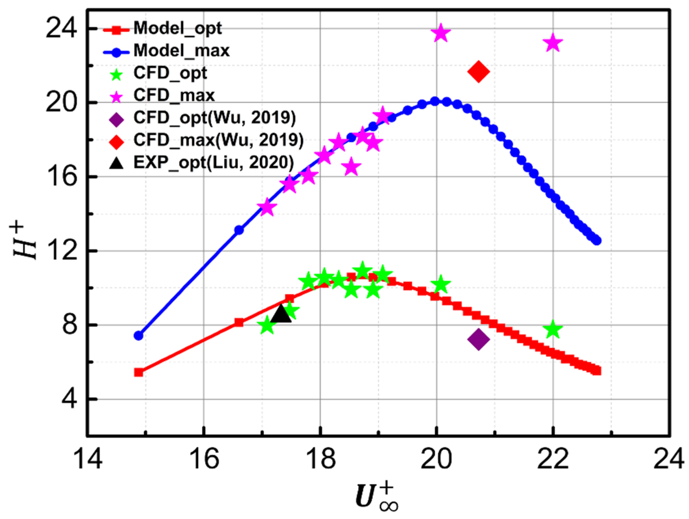
(3) The model results are consistent with the present numerical results and with previous data. For the solution of the optimal depth, the average error of the model is less than 4.35% when $U_{\infty }^{+}<20.07$ (Re < $2.18\times {10}^5$). For the solution of the maximum depth, the average error of the model is less than 4.09% when $U_{\infty }^{+}<19.07$ (Re <$1.31\times {10}^5$).

References

1. Fu, Z.; Liang, X.; Zhang, K. Asymmetrical Velocity Distribution in the Drag-Reducing Channel Flow of Surfactant Solution Caused by an Injected Ultrathin Water Layer. Symmetry 2020, 12, 846. [Google Scholar] [CrossRef]
2. Yu, J.C.; Wahls, R.A.; Esker, B.M.; Lahey, L.T.; Akiyama, D.G.; Drake, M.L.; Christensen, D.P. Total Technolo-gy Readiness Level: Accelerating Technology Readiness for Aircraft Design. In Proceedings of the AIAA AVIATION 2021 FORUM, Online, 2–6 August 2021; p. 2454. [Google Scholar]
3. Zhang, Y.; Chen, H.; Fu, S.; Dong, W. Numerical study of an airfoil with riblets installed based on large eddy simulation. Aerosp. Sci. Technol. 2018, 78, 661–670. [Google Scholar] [CrossRef]
4. Zhang, Y.; Chongyang, Y.; Haixin, C.; Yuhui, Y. Study of riblet drag reduction for an infinite span wing with different sweep angles. Chin. J. Aeronaut. 2020, 33, 3125–3137. [Google Scholar] [CrossRef]
5. Wu, Z.; Li, S.; Liu, M.; Wang, S.; Yang, H.; Liang, X. Numerical research on the turbulent drag reduction mechanism of a transverse groove structure on an airfoil blade. Eng. Appl. Comput. Fluid Mech. 2019, 13, 1024–1035. [Google Scholar] [CrossRef] [Green Version]
6. Walsh, M.J.; Weinstein, L.M. Drag and Heat-Transfer Characteristics of Small Longitudinally Ribbed Surfaces. AIAA J. 1979, 17, 770–771. [Google Scholar] [CrossRef]
7. DeGroot, C.; Wang, C.; Floryan, J.M. Drag Reduction Due to Streamwise Grooves in Turbulent Channel Flow. J. Fluids Eng. 2016, 138, 121201. [Google Scholar] [CrossRef]
8. Wainwright, D.K.; Fish, F.E.; Ingersoll, S.; Williams, T.M.; Leger, J.S.; Smits, A.J.; Lauder, G.V. How smooth is a dolphin? The ridged skin of odontocetes. Biol. Lett. 2019, 15, 20190103. [Google Scholar] [CrossRef]
9. Lang, A.; Afroz, F.; Motta, P.; Wilroy, J.; Wahidi, R.; Elliott, C.; Habegger, M.L. Sharks, Dolphins and Butterflies: Micro-Sized Surfaces Have Macro Effects. In Proceedings of the Fluids Engineering Division Summer Meeting. American Society of Mechanical Engineers, Waikoloa, HI, USA, 30 July–3 August 2017; p. V01CT21A001. [Google Scholar]
10. Abdulbari, H.A.; Mahammed, H.D.; Hassan, Z.B.Y. Bio-Inspired Passive Drag Reduction Techniques: A Review. ChemBioEng Rev. 2015, 2, 185–203. [Google Scholar] [CrossRef]
11. Asadzadeh, H.; Moosavi, A.; Etemadi, A. Numerical simulation of drag reduction in microgrooved substrates using lattice-Boltzmann method. J. Fluids Eng. 2019, 141, 071111. [Google Scholar] [CrossRef]
12. Walsh, M.J. Riblets as a Viscous Drag Reduction Technique. AIAA J. 1983, 21, 485–486. [Google Scholar] [CrossRef]
13. Rastegari, A.; Akhavan, R. The common mechanism of turbulent skin-friction drag reduction with superhydrophobic longitudinal microgrooves and riblets. J. Fluid Mech. 2018, 838, 68–104. [Google Scholar] [CrossRef]
14. Ran, W.; Zare, A.; Jovanović, M.R. Model-based design of riblets for turbulent drag reduction. J. Fluid Mech. 2020, 906, A7. [Google Scholar] [CrossRef]
15. Peet, Y.; Sagaut, P.; Charron, Y. Pressure loss reduction in hydrogen pipelines by surface restructuring. Int. J. Hydrogen Energy 2009, 34, 8964–8973. [Google Scholar] [CrossRef]
16. Li, L.; Zhu, J.; Li, J.; Song, H.; Zeng, Z.; Wang, G.; Zhao, W.; Xue, Q. Effect of vortex frictional drag reduction on ordered microstructures. Surf. Topogr. Metrol. Prop. 2019, 7, 025008. [Google Scholar] [CrossRef]
17. Liu, M.; Li, S.; Wu, Z.; Zhang, K.; Wang, S.; Liang, X. Entropy generation analysis for grooved structure plate flow. Eur. J. Mech.-B/Fluids 2019, 77, 87–97. [Google Scholar] [CrossRef]
18. Wang, L.; Wang, C.; Wang, S.; Sun, G.; You, B. Design and analysis of micro-nano scale nested-grooved surface structure for drag reduction based on ‘Vortex-Driven Design’. Eur. J. Mech.-B/Fluids 2020, 85, 335–350. [Google Scholar] [CrossRef]
19. Wood, D.H.; Antonia, R.A. Measurements in a Turbulent Boundary Layer over Ad-Type Surface Roughness. J. Appl. Mech. 1975, 42, 591–597. [Google Scholar] [CrossRef]
20. Choi, K.-S.; Fujisawa, N. Possibility of drag reduction usingd-type roughness. Flow Turbul. Combust. 1993, 50, 315–324. [Google Scholar] [CrossRef]
21. Bushnell, D. Turbulent drag reduction for external flows. In Proceedings of the 21st Aerospace Sciences Meeting, Reno, NV, USA, 10–13 January 1983. [Google Scholar]
22. Cui, J.; Fu, Y. A numerical study on pressure drop in microchannel flow with different bionic micro-grooved surfaces. J. Bionic Eng. 2012, 9, 99–109. [Google Scholar] [CrossRef]
23. Wang, B.; Wang, J.; Zhou, G.; Chen, D. Drag Reduction by Microvortexes in Transverse Microgrooves. Adv. Mech. Eng. 2014, 6, 734012. [Google Scholar] [CrossRef]
24. Chen, H.; Gao, Y.; Stone, H.A.; Li, J. “Fluid bearing” effect of enclosed liquids in grooves on drag reduction in microchannels. Phys. Rev. Fluids 2016, 1, 083904. [Google Scholar] [CrossRef]
25. Wang, J.; Ma, W.; Li, X.; Bu, W.; Liu, C. Slip theory-based numerical investigation of the fluid transport behavior on a surface with a biomimetic microstructure. Eng. Appl. Comput. Fluid Mech. 2019, 13, 609–622. [Google Scholar] [CrossRef]
26. Davies, J.; Maynes, D.; Webb, B.W.; Woolford, B. Laminar flow in a microchannel with superhydrophobic walls exhibiting transverse ribs. Phys. Fluids 2006, 18, 087110. [Google Scholar] [CrossRef]
27. Rothstein, J.P. Slip on Superhydrophobic Surfaces. Annu. Rev. Fluid Mech. 2010, 42, 89–109. [Google Scholar] [CrossRef]
28. Wang, B.; Wang, J.; Chen, D. A prediction of drag reduction by entrapped gases in hydrophobic transverse grooves. Sci. China Technol. Sci. 2013, 56, 2973–2978. [Google Scholar] [CrossRef]
29. Seo, S.-H.; Nam, C.-D.; Han, J.-Y.; Hong, C.-H. Drag reduction of a bluff body by grooves laid out by design of experiment. J. Fluids Eng. 2013, 135, 111202. [Google Scholar] [CrossRef]
30. Lang, A.W.; Jones, E.M.; Afroz, F. Separation control over a grooved surface inspired by dolphin skin. Bioinspir. Biomim. 2017, 12, 026005. [Google Scholar] [CrossRef] [PubMed]
31. Mariotti, A.; Buresti, G.; Salvetti, M. Separation delay through contoured transverse grooves on a 2D boat-tailed bluff body: Effects on drag reduction and wake flow features. Eur. J. Mech.-B/Fluids 2018, 74, 351–362. [Google Scholar] [CrossRef]
32. Liu, W.; Ni, H.; Wang, P.; Zhou, Y. An investigation on the drag reduction performance of bioinspired pipeline surfaces with transverse microgrooves. Beilstein J. Nanotechnol. 2020, 11, 24–40. [Google Scholar] [CrossRef] [PubMed] [Green Version]
33. Breuer, M.; Jovičić, N. Separated flow around a flat plate at high incidence: An LES investigation. J. Turbul. 2001, 2, N18. [Google Scholar] [CrossRef]
34. Martin, S.; Bhushan, B. Fluid flow analysis of a shark-inspired microstructure. J. Fluid Mech. 2014, 756, 5–29. [Google Scholar] [CrossRef]
35. Hemida, H.; Gil, N.; Baker, C.; Baker, C. LES of the Slipstream of a Rotating Train. J. Fluids Eng. 2010, 132, 051103. [Google Scholar] [CrossRef]
36. Meneveau, C.; Lund, T.S.; Cabot, W.H. A Lagrangian dynamic subgrid-scale model of turbulence. J. Fluid Mech. 1996, 319, 353–385. [Google Scholar] [CrossRef] [Green Version]
37. Rhie, C.M.; Chow, W.L. Numerical study of the turbulent flow past an airfoil with trailing edge separation. AIAA J. 1983, 21, 1525–1532. [Google Scholar] [CrossRef]
38. Zhang, Z.; Zhang, M.; Cai, C.; Kang, K. A general model for riblets simulation in turbulent flows. Int. J. Comput. Fluid Dyn. 2020, 34, 333–345. [Google Scholar] [CrossRef]
39. Ahmadi-Baloutaki, M.; Carriveau, R.; Ting, D.S.-K. Effect of free-stream turbulence on flow characteristics over a transversely-grooved surface. Exp. Therm. Fluid Sci. 2013, 51, 56–70. [Google Scholar] [CrossRef]
40. Song, X.-W.; Zhang, M.-X.; Lin, P.-Z. Skin Friction Reduction Characteristics of Nonsmooth Surfaces Inspired by the Shapes of Barchan Dunes. Math. Probl. Eng. 2017, 2017, 6212605. [Google Scholar] [CrossRef]
41. Currie, I.G. Fundamental Mechanics of Fluids; CRC Press: Boca Raton, FL, USA, 2016. [Google Scholar]
42. Fukagata, K.; Kasagi, N.; Koumoutsakos, P. A theoretical prediction of friction drag reduction in turbulent flow by superhydrophobic surfaces. Phys. Fluids 2006, 18, 051703. [Google Scholar] [CrossRef]
43. Dean, R.B. Reynolds Number Dependence of Skin Friction and Other Bulk Flow Variables in Two-Dimensional Rectangular Duct Flow. J. Fluids Eng. 1978, 100, 215–223. [Google Scholar] [CrossRef]
44. Min, T.; Kim, J. Effects of hydrophobic surface on skin-friction drag. Phys. Fluids 2004, 16, L55–L58. [Google Scholar] [CrossRef]
45. Feng, B.; Chen, D.; Wang, J.; Yang, X. Bionic Research on Bird Feather for Drag Reduction. Adv. Mech. Eng. 2014, 7. [Google Scholar] [CrossRef]
Figure 1. Computational domain and boundary conditions.
Symmetry 14 00342 g001
Figure 2. Mesh distribution around transverse V-grooves.
Symmetry 14 00342 g002
Figure 3. Verification of grid independence.
Symmetry 14 00342 g003
Figure 4. The comparison of numerical and experimental results. Mean velocity profile over the grooved plate when the turbulence intensity is 0.4% (a) and 4.4% (b); The instantaneous velocity vector over the grooved plate of experimental data [40] (c) and numerical result (d).
Symmetry 14 00342 g004aSymmetry 14 00342 g004b
Figure 5. Total drag-reduction rate versus depth (AR = 2).
Symmetry 14 00342 g005
Figure 6. Velocity distribution in grooves.
Symmetry 14 00342 g006
Figure 7. Pressure (left) and wall shear stress (right) distribution in grooves.
Symmetry 14 00342 g007
Figure 8. Drag reduction rate versus (a) slip velocity; (b) local friction velocity; (c) dimensionless slip velocity.
Symmetry 14 00342 g008aSymmetry 14 00342 g008b
Figure 9. Process of model construction.
Symmetry 14 00342 g009
Figure 10. Schematic diagram of velocity profiles within the groove.
Symmetry 14 00342 g010
Figure 11. The position of boundary vortex varies with dimensionless velocity.
Symmetry 14 00342 g011
Figure 12. Boltzmann fitting of K value.
Symmetry 14 00342 g012
Figure 13. Comparison of the results of Equation (12) with CFD data.
Symmetry 14 00342 g013
Figure 14. The velocity profile over the grooved plate is the superposition of slip velocity and no-slip flow velocity profile.
Symmetry 14 00342 g014
Figure 15. The velocity profile of U g and U g s ( U + = 22 ,   h = 0.1 ).
Symmetry 14 00342 g015
Figure 16. Comparison of the results of Equation (18) with CFD data and experimental data.
Symmetry 14 00342 g016
Figure 17. Gauge pressure distribution (the atmospheric pressure is 101,325 pa).
Symmetry 14 00342 g017
Figure 18. Schematic diagram of p ( x ) .
Symmetry 14 00342 g018
Figure 19. Comparison of the results of Equation (25) with CFD data.
Symmetry 14 00342 g019
Figure 20. Steps for solving Equation (26).
Symmetry 14 00342 g020
Figure 21. The dimensionless depths predicted by the model versus dimensionless inflow velocities.
Symmetry 14 00342 g021
Figure 22. The groove depths predicted by the model versus local Reynolds numbers.
Symmetry 14 00342 g022
Figure 23. Schematic diagram of three grooved plates with different groove depths.
Symmetry 14 00342 g023
Figure 24. Time-averaged entropy generation over different plates.
Symmetry 14 00342 g024