Estimation and Testing of Wilcoxon–Mann–Whitney Effects in Factorial Clustered Data Designs

Abstract

Clustered data arise frequently in many practical applications whenever units are repeatedly observed under a certain condition. One typical example for clustered data are animal experiments, where several animals share the same cage and should not be assumed to be completely independent. Standard methods for the analysis of such data are Linear Mixed Models and Generalized Estimating Equations—however, checking their assumptions is not easy, especially in scenarios with small sample sizes, highly skewed, count, and ordinal or binary data. In such situations, Wilcoxon–Mann–Whitney type effects are suitable alternatives to mean-based or other distributional approaches. Hence, no specific data distribution, symmetric or asymmetric, is required. Within this work, we will present different estimation techniques of such effects in clustered factorial designs and discuss quadratic- and multiple contrast type-testing procedures for hypotheses formulated in terms of Wilcoxon–Mann–Whitney effects. Additionally, the framework allows for the occurrence of missing data: estimation and testing hypotheses are based on all-available data instead of complete-cases. An extensive simulation study investigates the precision of the estimators and the behavior of the test procedures in terms of their type-I error control. One real world dataset exemplifies the applicability of the newly proposed procedures.

1. Introduction

Clustered data are commonly encountered in medical research and various disciplines and occur whenever a subject is not only observed once under a certain condition, but multiple times. For instance, animals sharing the same cage, students in classes, skin irritations, etc., are different examples of clustered data. In these situations, subjects provide multiple possibly dependent observations (not necessarily equally sized). Standard methods for the analysis of independent observations (e.g., t-test, linear regression, Analysis of Variance (ANOVA), etc.) are not applicable in such scenarios. Ignoring that structure might result in bias (such as inflated type-I error rates and estimation bias) and therefore appropriate models are necessary for making inference. Reducing the clusters to a single point by, e.g., computing their mean or median, typically results in a loss of power and decreased precision of point estimates [1,2,3]. Furthermore, estimation of treatment effects becomes an issue because of presence of intra-cluster correlations and unequally sized clusters, see, e.g., Gao [4]. Under certain assumptions such as multivariate normality and linear relationships, Linear Mixed Models and Generalized Estimating Equations can be used. However, testing these assumptions is difficult in practice as noted by Fitzmaurice et al. [5] and Johnson and Wichern [6], especially when dealing with small sample sizes. Further, if count, ordinal, or highly skewed data are present, mean-based approaches are not applicable and thus, another type of measure is needed. On the contrary, Wilcoxon–Mann–Whitney-type effects $p=P(X<Y)+\frac{1}{2}P(X=Y)$ [7] are purely non-parametric quantities, which can be used for the definition of a treatment effect for metric, discrete, ordinal, and even dichotomous data in a unified way. Thus, the response variable is not assumed to be symmetrically distributed. Here X and Y represent two independent random variables coming from different populations. In the literature, p is also called relative effect [8] or probabilistic index [9,10], see Brunner et al. [11] for an overview. It is the aim of this paper to discuss different estimation techniques of such effects in factorial repeated measures designs with a clustered structure. We hereby differ between non-informative and informative cluster sizes by presenting weighted and unweighted estimators. Here, informative cluster sizes mean that the cluster sizes might be related to the outcome. In addition to estimation, we further introduce different statistical inference methods for testing hypotheses formulated in terms of these effects. All methods allow for the occurrence of missing data and take all-available data into consideration, which is a novelty since previous methods by Akritas et al. [12], Fong et al. [13], Domhof et al. [14] and Amro et al. [15] can only be used for testing hypotheses in terms of distribution functions in scenarios with missing data and do not allow for clustered data. Akritas and Brunner [16] and Brunner et al. [17] propose ranking procedures for testing hypotheses green formulated in terms of distribution functions in clustered data designs, see Brunner et al. [18] for an excellent overview. Thus, the aim of this work is to provide a framework for estimating Wilcoxon–Mann–Whitney-type effects, as well as to present test procedures for hypotheses formulated in terms of these effects in factorial repeated measures designs with clustered data. The paper is organized as follows. First, a real world example is introduced in Section 2 that motivates the development of the methods. Next, in Section 3 the factorial repeated measures model with a clustered data structure is introduced. Subsequently, point estimators and their asymptotic distributions are derived in Section 4 and Section 5. Further, test procedures and multiple hypotheses in this framework are presented in Section 6 and Section 7. The results of extensive simulation studies are presented in the following Section 8. Finally, the motivating example is analyzed by using the newly proposed methods in Section 9 and a discussion and conclusion about the findings is given in Section 10. All proofs can be found in the Appendix A.

2. Motivating Example

In order to motivate the development of methods for factorial repeated measures data with a clustered structure, we consider the secondary/exploratory outcome analysis of retinal thickness in the ’Sunphenon in progressive forms of multiple sclerosis’ (SUPREMES) trial by Klumbies et al. [19], which was a relatively small clinical trial in progressive multiple sclerosis (MS) patients. MS is the most common autoimmune disorder of the central nervous system, affecting approximately 2.8 million people worldwide [20]. In MS, immune cells attack the myelin sheaths of nerve fibers, often resulting in neurodegeneration and thus permanent disability. In most cases, the disease starts with a relapsing–remitting course, followed by a progressive course around 15–20 years after diagnosis. Around 15% of patients feature a progressive course from onset of the disease [21]. MS is associated with visual impairment caused by optic nerve and posterior visual pathway damage, which can be quantified with optical coherence tomography based thickness measurements of the retinal nerve fiber layer, the combined ganglion cell, and inner plexiform layer (GCIP) and inner nuclear layer (INL) [22]. Retinal thickness analysis has been suggested as an outcome parameter in MS clinical trials [23]. In animal models of MS, epigallocatechin gallate (EGCG), which is an anti-inflammatory agent, indicated neuroprotective properties. The recent paper of Klumbies et al. [19] investigated the effect of EGCG on retinal thickness as an indicator for treatment response in progressive MS. For this motivating example, only the parameter peripapillary retinal nerve fiber layer (pRNFL) will be investigated. Longitudinal OCT data were available from 31 patients, from which 15 patients were assigned to the intervention group and 16 to the control group, respectively. For most patients, both eyes were investigated, thus leading to possibly dependent observations, since assuming independence of the eyes from the same patient would be dubious. Further, missing values occur: From 61 patients in the SUPREMES trial, only 31 contributed to the final analysis and at 3-year follow-up, only 8 patients remained in the study.

Table 1. Number of patients with pRNFL measurements in each group at baseline, 1-year follow-up, 2-year follow-up, and 3-year follow-up.

Group	First OCT	1-Year F/U	2-Year F/U	3-Year F/U
Verum	15	14	7	3
Placebo	16	16	11	5

displays the numbers of patients with pRNFL measurements in each group at each time point. Due to the extremely small number of measurements after 3 years, this time point was discarded from the analysis.

Since the sample size was quite small and many missing values occurred, the authors tested—besides other hypotheses—whether there exists a statistical interaction of treatment and time using non-parametric analysis of longitudinal data in factorial experiments, as proposed by Brunner et al. [18]. One disadvantage of this procedure is that it cannot handle missing values and a clustered data structure. Therefore, Klumbies et al. [19] conducted a complete-case analysis and modeled the eyes as a second sub-plot factor besides the sub-plot factor time. In order to close this methodological gap, a general factorial model with repeated measurements, allowing for possibly correlated dependent replicates will be introduced in the next section.

3. The Factorial Repeated Measures Model with Missing Values

First, we study the general factorial repeated measures model without a clustered structure with independent random vectors

$$\begin{array}{ccc}\hfill {\mathit{X}}_{ik}& =& {\left(\left({\lambda }_{i1k},X_{i1k}\right),\dots ,\left({\lambda }_{idk},X_{idk}\right)\right)}^{\prime },i=1,\dots ,a;k=1,\dots ,n_i,\mathrm{with}\hfill \\ \hfill {\lambda }_{isk}& =& \left\{\begin{array}{cc}1,& X_{isk}\mathrm{is}\mathrm{observed}\\ 0,& X_{isk}\mathrm{is}\mathrm{missing}.\end{array}\right.\hfill \end{array}$$

(1)

Here, the random variable $X_{isk}\sim F_{is},i=1,\dots ,a;s=1,\dots ,d;k=1,\dots ,n_i$ represents the s-th repeated measurement of the k-th subject in group i.

To account for metric, discrete, ordinal and ordered categorical data in a unified way, we use the normalized version of the distribution function

$$F_{is}\left(x\right)=P(X_{isk}<x)+\frac{1}{2}P(X_{isk}=x),$$

which is the average of the left and the right continuous version of the distribution function $F_{is}^{-}=P(X_{is1}<x)$ and $F_{is}^{+}=P(X_{is1}\le x)$, which was first introduced by Ruymgaart [24].

In model (1), the numbers of non-missing observations under time-point s in group i, the overall sample size and the minimal number of observations over all groups and time points are given by

$$\begin{array}{c}\hfill {\lambda }_{is}=\sum _{k=1}^{n_i}{\lambda }_{isk},N=\sum _{i=1}^a{n}_i\mathrm{and}{\lambda }_{min}=min({\lambda }_{11},\cdots ,{\lambda }_{ad}).\end{array}$$

We propose to use unweighted relative effects

$$p_{is}=\int Gd{F}_{is}=P(Z<X_{is1})+\frac{1}{2}P(Z=X_{is1}),i=1,\dots ,a;s=1,\dots ,d,$$

(2)

with $G=\frac{1}{ad}{\sum }_{i=1}^a{\sum }_{s=1}^d{F}_{is}$ being the unweighted mean distribution function and $Z\sim G$, independent of $X_{isk}$. The relative effect $p_{is}$ models the relationship of the distribution $F_{is}$ to the average distribution G. If $p_{is}>p_{jt}$, then data coming from $F_{is}$ tend to be larger than data coming from $F_{jt}$. If $p_{is}=p_{jt}$, then there is no tendency to greenlarger nor smaller values between the two distributions. For more information on unweighted and weighted relative effects, we refer to Brunner et al. [25] and Brunner et al. [26]. In the following, we always refer to unweighted relative effects, if relative effects are mentioned.

General Factorial Model with Clustered Data

In the following we introduce a general factorial longitudinal model with clustered data. In comparison with model (1), we observe random vectors ${\mathit{X}}_{ik}={({\mathit{X}}_{i1k},..,{\mathit{X}}_{idk})}^{\prime }$ with

$$\begin{array}{cc}\hfill & {\mathit{X}}_{isk}={\left({\lambda }_{isk},\left(X_{isk1},\dots ,X_{isk{m}_{isk}}\right)\right)}^{\prime },\mathrm{where}\hfill \\ \hfill & X_{isku}\sim F_{is},u=1,\dots ,m_{isk},\hfill \end{array}$$

(3)

and $m_{isk}$ denotes the number of possibly dependent replicates of subject k in group i at time s and $m_{is}={\sum }_{k=1}^{n_i}{m}_{isk}{\lambda }_{isk}$ denotes the total number of possibly dependent replicates in group i at time s. Thus, the number of dependent replicates may vary for each subject and may not be under experimental control. Note, that we do not assume any correlation structure of the dependent replicates. Similarly as in (2), we define the relative effect as

$$\begin{array}{cc}\hfill p_{is}& =\int Gd{F}_{is}=P(Z<X_{is11})+\frac{1}{2}P(Z=X_{is11})\hfill \end{array}$$

with

$$F_{is}\left(x\right)=P(X_{isku}<x)+\frac{1}{2}P(X_{isku}=x).$$

Note, that model (1) is contained within this model as a special case with $m_{isk}\equiv 1$. In order to derive asymptotic results, we impose the following model assumptions:

Assumption A1.

• A1.1: $\frac{n_i}{N}\to {\kappa }_i\in (0,1]$;
• A1.2: $N\to \infty$ such that $\frac{N}{{\lambda }_{min}}<N_0$, $N_0$ being a fixed constant;
• A1.3: $N\to \infty$ such that $m_{is}<M_0$, $M_0$ being a fixed constant.

Assumption A1.1 ensures that none of the groups vanishes asymptotically, whereas Assumptions A1.2 and A1.3 ensure that the total sample size N and number of clustered observations $m_{is}$ is bounded. In the following section, estimators for the relative effect $\mathbf{p}$ will be derived.

4. Estimators and Their Asymptotic Distributions

We will first study estimators of relative effects in factorial repeated measures designs without clustered data (i.e., $m_{isk}\equiv 1$). In order to account for possible missing values, we define the empirical distribution function of the data under time point s in group i as the average of the all-available data by

$${\widehat{F}}_{isk}\left(x\right)=c(x-X_{isk}){\lambda }_{isk}\mathrm{resulting}\mathrm{in}{\widehat{F}}_{is}\left(x\right)=\frac{1}{{\lambda }_{is}}\sum _{k=1}^{n_i}{\widehat{F}}_{isk}\left(x\right).$$

Here, $c\left(u\right)=0,\frac{1}{2},1$, if $u<,=,>0$. By plugging in the empirical counterparts ${\widehat{F}}_{is}$, we obtain

$$\widehat{G}\left(x\right)=\frac{1}{ad}\sum _{i=1}^a\sum _{s=1}^d{\widehat{F}}_{is}\left(x\right),$$

$${\widehat{p}}_{is}=\int \widehat{G}d{\widehat{F}}_{is}=\frac{1}{{\lambda }_{is}}\sum _{k=1}^{n_i}\frac{{\lambda }_{isk}}{ad}\sum _{j=1}^a\sum _{t=1}^d\sum _{\ell =1}^{n_j}\frac{{\lambda }_{jt\ell }}{{\lambda }_{jt}}c(X_{isk}-X_{jt\ell })$$

(4)

and define

$$\widehat{\mathit{p}}={({\widehat{p}}_{11},\cdots ,{\widehat{p}}_{1d},{\widehat{p}}_{21},\cdots {\widehat{p}}_{ad})}^{\prime }.$$

4.1. Effect Estimation in Factorial Designs with Clustered Data

To generalize the estimation of empirical distribution functions and relative effects to the case of clustered data, we follow the idea of Roy et al. [1] who proposed two different approaches for estimating the distribution functions by using the cluster sizes as weighting schemes. In the first version of the estimator of the relative effect $\mathit{p}$, larger clusters add more weight to the estimation than smaller ones and in the second version, all clusters add the same weight to the estimation, disregarding their size. Analogously to Roy et al. [1] the estimators are called unweighted and weighted estimators, respectively. Note that Obuchowski [27] also used the weighted version in the two-sample case.

The two different versions of the empirical distribution functions (unweighted and weighted) are defined as follows:

$$\begin{array}{cc}\hfill & {\widehat{F}}_{is}^{\left({\upsilon }_1\right)}\left(x\right)=\frac{1}{{\lambda }_{is}}\sum _{k=1}^{n_i}\frac{1}{m_{isk}}\sum _{u=1}^{m_{isk}}c(x-X_{isku}){\lambda }_{isk}\hfill \\ \hfill & {\widehat{F}}_{is}^{\left({\upsilon }_2\right)}\left(x\right)=\frac{1}{m_{is}}\sum _{k=1}^{n_i}\sum _{u=1}^{m_{isk}}c(x-X_{isku}){\lambda }_{isk}.\hfill \end{array}$$

${\widehat{F}}_{is}^{\left({\upsilon }_1\right)}\left(x\right)$ is the unweighted estimator of $F_{is}\left(x\right)$, where the average of the count function is calculated separately for each cluster and these averages are then again averaged. ${\widehat{F}}_{is}^{\left({\upsilon }_2\right)}\left(x\right)$ is the weighted estimator of $F_{is}\left(x\right)$ where the counts are averaged over all observations.

In order to write the estimators in a unified way, we define weights

$$w_{isk}^{{\upsilon }_1}=\frac{1}{{\lambda }_{is}{m}_{isk}}\mathrm{and}{w}_{isk}^{{\upsilon }_2}=\frac{1}{m_{is}},$$

then an estimator for $F_{is}\left(x\right)$ and $G\left(x\right)$ is given by

$${\widehat{F}}_{is}^{*}\left(x\right)=\sum _{k=1}^{n_i}\sum _{u=1}^{m_{isk}}{w}_{isk}^{*}c(x-X_{isku}){\lambda }_{isk},*\in \{{\upsilon }_1,{\upsilon }_2\}$$

and

$${\widehat{G}}^{*}=\frac{1}{ad}\sum _{i=1}^a\sum _{s=1}^d{\widehat{F}}_{is}^{*}=\frac{1}{ad}\sum _{i=1}^a\sum _{s=1}^d\sum _{k=1}^{n_i}{\lambda }_{isk}\sum _{u=1}^{m_{isk}}{w}_{isk}^{*}c(x-X_{isku}).$$

It then follows that an estimator of $p_{is}$ is given by

$$\begin{array}{cc}\hfill {\widehat{p}}_{is}^{*}& =\int {\widehat{G}}^{*}d{\widehat{F}}_{is}^{*}=\frac{1}{ad}\sum _{j=1}^a\sum _{t=1}^d\sum _{k=1}^{n_i}\sum _{u=1}^{m_{isk}}{\lambda }_{isk}{w}_{isk}^{*}{\widehat{F}}_{jt}^{*}\left(X_{isku}\right)\hfill \end{array}$$

(5)

$$\begin{array}{cc}\hfill & =\frac{1}{ad}\sum _{k=1}^{n_i}\sum _{j=1}^a\sum _{t=1}^d\sum _{\ell =1}^{n_j}\sum _{u=1}^{m_{isk}}\sum _{v=1}^{m_{jt\ell }}{\lambda }_{isk}{\lambda }_{jt\ell }{w}_{isk}^{*}{w}_{jt\ell }^{*}c(X_{isku}-X_{jt\ell v}).\hfill \end{array}$$

(6)

Note that in order to derive the theory of these estimators, the weights need to fulfill the following properties

Proposition 1.

If Assumption A1.3 is fulfilled, it holds that

• A2.1: ${\lambda }_{isk}{w}_{isk}^{*}{m}_{isk}\le \mathcal{O}\left(\frac{1}{{\lambda }_{min}}\right)$;
• A2.2: ${\sum }_{k=1}^{n_i}{\lambda }_{isk}{w}_{isk}^{*}{m}_{isk}=1$.

Furthermore note, that the application of all weights which fulfill both properties is theoretically possible. For example, Zou [28] developed an ’optimal’ estimator, which incorporates information on cluster sizes and intra-cluster correlations by a mixed model approach.

First, we will study the asymptotic properties of general estimators for $\mathit{p}$ in the following proposition.

Proposition 2.

The estimator ${\widehat{\mathit{p}}}^{*}={\left({\widehat{p}}_{11}^{*},\cdots ,{\widehat{p}}_{1d}^{*},{\widehat{p}}_{21}^{*},\cdots ,{\widehat{p}}_{ab}^{*}\right)}^{\prime }$ is asymptotically unbiased and strongly consistent, i.e.,

• $E\left({\widehat{\mathit{p}}}^{*}\right)=\mathit{p}+\mathcal{O}\left(\frac{1}{{\lambda }_{min}}\right)$;
• $\widehat{\mathit{p}}-\mathit{p}\stackrel{a.s.}{\to }0,{\lambda }_{min}\to \infty$.

Subsequently, the asymptotic distribution of the statistic $\sqrt{N}\left({\widehat{\mathit{p}}}^{*}-\mathit{p}\right)$ will be derived. It will be indicated in the next theorem that $\sqrt{N}\left({\widehat{\mathit{p}}}^{*}-\mathit{p}\right)$ has asymptotically under A1.1 and A1.2, the same distribution as the random vector $\sqrt{N}{\mathit{B}}^{*}$, with

$$\begin{array}{c}\hfill \sqrt{N}{\mathit{B}}^{*}=\sum _{h=1}^a\sqrt{N}{\mathit{B}}_h^{*}=\sum _{h=1}^a\left(\frac{\sqrt{N}}{n_h}\sum _{k=1}^{n_h}\left({\mathbf{\Psi }}_{hk}^{*}-E\left({\mathbf{\Psi }}_{hk}^{*}\right)\right)\right)\end{array}$$

based on random variables defined as

$${\mathsf{\Psi }}_{is,hk}^{*}:=\left\{\begin{array}{c}-\frac{n_h}{ad}\sum _{t=1}^d\sum _{u=1}^{m_{htk}}{\lambda }_{htk}{w}_{htk}^{*}{F}_{is}\left(X_{htku}\right),\mathrm{for}h\ne i\hfill \\ \frac{n_h}{ad}\sum _{j\ne i}^a\sum _{t=1}^d\sum _{u=1}^{m_{isk}}{\lambda }_{isk}{w}_{isk}^{*}{F}_{jt}\left(X_{isku}\right)\hfill \\ +\frac{n_h}{ad}\sum _{t=1}^d(\sum _{u=1}^{m_{isk}}{\lambda }_{isk}{w}_{isk}^{*}{F}_{it}\left(X_{isku}\right)\hfill \\ -\sum _{u=1}^{m_{itk}}{\lambda }_{itk}{w}_{itk}^{*}{F}_{is}\left(X_{itku}\right)),\mathrm{else}.\hfill \end{array}\right.$$

The expectation of ${\mathbf{\Psi }}_{hk}^{*}$ can be written as

$${\beta }_{is,ik}^{*}:=E\left({\mathsf{\Psi }}_{is,hk}^{*}\right)=\left\{\begin{array}{c}-\frac{n_h}{ad}\sum _{t=1}^d{\lambda }_{htk}{m}_{htk}{w}_{htk}^{*}{p}^{(is,ht)},\mathrm{for}h\ne i\hfill \\ \frac{n_h}{ad}\sum _{j\ne i}^a\sum _{t=1}^d{m}_{isk}{\lambda }_{isk}{w}_{isk}^{*}{p}^{(jt,is)})\hfill \\ +\frac{n_h}{ad}\sum _{t=1}^d(m_{isk}{\lambda }_{isk}{w}_{isk}^{*}{p}^{(it,is)}\hfill \\ -m_{itk}{\lambda }_{itk}{w}_{itk}^{*}{p}^{(is,it)}),\mathrm{else},\hfill \end{array}\right.$$

with $p^{(is,ht)}:=\int F_{is}d{F}_{ht}$ denoting pairwise relative effects between groups i and h and time points s and t.

Theorem 1.

Let $\sqrt{N}{\mathit{B}}^{*}={\sum }_{h=1}^a\sqrt{N}{\mathit{B}}_h^{*}={\sum }_{h=1}^a\sqrt{N}{\left(B_{11,h}^{*},\cdots ,B_{ad,h}^{*}\right)}^{\prime }$ be the vector of the random variables $\sqrt{n}{B}_{is}$, $i=1,\cdots ,d$; $s=1,\cdots ,d$. If A1.1 and A1.2 hold true, then

$$||\sqrt{N}\left({\widehat{\mathit{p}}}^{*}-\mathit{p}\right)-\sqrt{N}{\mathit{B}}^{*}{||}_2^2=\mathcal{O}\left(\frac{1}{N}\right).$$

It follows that the asymptotic covariance matrix of $\sqrt{N}\left({\widehat{\mathit{p}}}^{*}-\mathit{p}\right)$ is given by

$${\mathit{V}}_N^{*}=Cov\left(\sqrt{N}{\mathit{B}}^{*}\right).$$

The asymptotic multivariate normality of the linear statistic $\sqrt{N}\left({\widehat{\mathit{p}}}^{*}-\mathit{p}\right)$ is given in the next theorem.

Theorem 2.

Under Assumptions A1.1 and A1.2, the statistic $\sqrt{N}\left({\widehat{\mathit{p}}}^{*}-\mathit{p}\right)$ follows asymptotically, as $N\to \infty$, a multivariate normal distribution with expectation $\mathbf{0}$ and covariance matrix ${\mathit{V}}_N^{*}$.

However, this covariance matrix is mostly unknown in practical applications and must be estimated in order to be able to make statistical inferences. In Section 5 we will derive a consistent and positive semi-definite estimator of the covariance matrix.

4.2. Informative Cluster Sizes

In many applications, the cluster sizes $m_{isk}$ (might) depend on the outcome of interest, i.e.,

Assumption 2.

$$E\left(X_{isku}\right)\ne E\left(X_{isku}\right|m_{isk}),i=1,\dots ,a;s=1,\dots ,d;k=1,\dots ,n_i;u=1,\dots ,m_{isk}.$$

Which makes them non-ignorable or informative [29]. As an example, consider the periodontal disease (an inflammation of the gums and bone that surround and support the teeth) study [30]. Severe periodontitis ends in the falling out of teeth and, thus, cluster sizes (patient’s teeth) depend on the clinical outcome. Hoffmann et al. [29], among others, suggest a Within-Cluster-Resampling (WCR) method for the analysis of informative clustered binary data. This approach is also applicable in the rather general model considered here and will be described in the following:

A randomly chosen observation $X_{isk}^q$ is sampled from cluster ${\mathit{X}}_{isk}$. This is done for each of all $N*d$ clusters, resulting in a dataset involving single observations only. The latter is repeated Q times, e.g., Q = 10,000, and for each of the Q datasets, the vector of relative effects $\mathbf{p}$ is estimated by adapting Equation (4):

$${\widehat{p}}_{is}^{\mathsf{\Delta },q}=\frac{1}{{\lambda }_{is}}\sum _{k=1}^{n_i}\frac{{\lambda }_{isk}}{ad}\sum _{j=1}^a\sum _{t=1}^d\sum _{\ell =1}^{n_j}\frac{{\lambda }_{jt\ell }}{{\lambda }_{jt}}c(X_{isk}^q-X_{jt\ell }^q).$$

An estimator and its asymptotic distribution is given in the following theorem.

Theorem 3.

Let

$${\widehat{\mathit{p}}}^{\mathsf{\Delta }}=\frac{1}{Q}\sum _{q=1}^Q{\widehat{\mathit{p}}}^{\mathsf{\Delta },q}$$

denote the Within-Cluster-Resampling based estimator. If $N\to \infty$, then

$$\sqrt{N}\left({\widehat{\mathit{p}}}^{\mathsf{\Delta }}-\mathit{p}\right)\to \mathcal{N}(\mathbf{0},{\mathbf{\Sigma }}^{\mathsf{\Delta }}),$$

where ${\mathbf{\Sigma }}^{\mathsf{\Delta }}$ is finite.

A consistent variance is estimator is provided in the next theorem.

Theorem 4.

Let N and ${\widehat{\mathit{p}}}^{\mathsf{\Delta }}$ be defined as in Theorem 3. Then, an estimator of ${\mathbf{\Sigma }}^{\mathsf{\Delta }}$ is given by

$${\widehat{\mathbf{\Sigma }}}^{\mathsf{\Delta }}=\widehat{Var}\left(\sqrt{N}\left({\widehat{\mathit{p}}}^{\mathsf{\Delta }}-\mathit{p}\right)\right)=N\left(\frac{1}{Q}\sum _{q=1}^Q{\widehat{\mathbf{\Sigma }}}_q-\frac{Q-1}{Q}{\mathit{S}}_{\mathit{p}}^2\right),$$

(7)

where ${\widehat{\mathbf{\Sigma }}}_q$ is the estimated covariance matrix from the q-th analysis (see the following chapter for the derivation of an estimator) and

$${\mathit{S}}_{\mathit{p}}^2=\frac{1}{Q-1}\sum _{q=1}^Q\left({\widehat{\mathit{p}}}^{\mathsf{\Delta },q}-{\widehat{\mathit{p}}}^{\mathsf{\Delta }}\right){\left({\widehat{\mathit{p}}}^{\mathsf{\Delta },q}-{\widehat{\mathit{p}}}^{\mathsf{\Delta }}\right)}^{\prime }$$

is the estimated covariance matrix among the Q resample-based estimates ${\widehat{\mathit{p}}}^{\mathsf{\Delta },q}$. Then, ${\widehat{\mathbf{\Sigma }}}^{\mathsf{\Delta }}$ is consistent for $\mathbf{\Sigma }=Var\left(\sqrt{N}\left({\widehat{\mathit{p}}}^{\mathsf{\Delta }}-\mathit{p}\right)\right)$.

The proofs of Theorem 3 and 4 can be found in the appendix of Hoffmann et al. [29]. The WCR-approach proposed by Hoffmann et al. [29] is computationally intensive and could possibly lead to negative variance estimators due to the subtraction in the variance estimation in Equation (7). Hoffmann et al. [29] noted, that this occurs rarely and concluded that in these scenarios, the number of resampled datasets Q or the number of clusters N may be too small for making inferences. However, the WCR-based approach is equivalent to the unweighted estimation of the relative effects $\mathit{p}$ as proposed by Roy et al. [1]—in both analysis all clusters are given equal weight, regardless of their size. Thus, the use of the unweighted estimator should be preferred over the WCR-based approach since its computation is less intensive and always leads to positive variance estimators. However, it should be noted that Assumption 2 of ignorable cluster-sizes is never imposed during the development of the theory in this work. Therefore, all weighting schemes that fulfill Assumptions A2.1 and A2.2 can be applied in case of non-ignorable cluster sizes-however, the resulting estimators have a different interpretation.

5. Estimation of the Covariance Matrix

Now, an estimator of the covariance matrix ${\mathit{V}}_N^{*}$ is derived. Similarly, as in Rubarth et al. [31], the random variables ${\mathsf{\Psi }}_{is,hk}^{*}$ are not observable. Otherwise, an estimator of ${\mathit{V}}_N^{*}$ would be given by

$${\tilde{\mathit{V}}}_N^{*}=\sum _{h=1}^a\frac{N}{n_h}{\tilde{\mathit{V}}}_{N,h}^{*}$$

with ${\tilde{\mathit{V}}}_{N,h}^{*}=\frac{1}{n_h-1}{\sum }_{k=1}^{n_h}\left({\mathbf{\Psi }}_{hk}^{*}-{\mathit{\beta }}_{hk}^{*}\right){\left({\mathbf{\Psi }}_{hk}^{*}-{\mathit{\beta }}_{hk}^{*}\right)}^{\prime }$. Therefore, we replace the unknown ${\mathsf{\Psi }}_{is,hk}^{*}$ with observable random variables. Define the vectors ${\widehat{\mathbf{\Psi }}}_{hk}^{*}={\left({\widehat{\mathsf{\Psi }}}_{11,hk}^{*},\cdots ,{\widehat{\mathsf{\Psi }}}_{ad,hk}^{*}\right)}^{\prime }$ with

$${\widehat{\mathsf{\Psi }}}_{is,hk}^{*}:=\left\{\begin{array}{c}-\frac{n_h}{ad}\sum _{t=1}^d\sum _{u=1}^{m_{htk}}{\lambda }_{htk}{w}_{htk}^{*}{\widehat{F}}_{is}^{*}\left(X_{htku}\right),\mathrm{for}h\ne i\hfill \\ \frac{n_h}{ad}\sum _{j\ne i}^a\sum _{t=1}^d\sum _{u=1}^{m_{isk}}{\lambda }_{isk}{w}_{isk}^{*}{\widehat{F}}_{jt}^{*}\left(X_{isku}\right)\hfill \\ +\frac{n_h}{ad}\sum _{t=1}^d(\sum _{u=1}^{m_{isk}}{\lambda }_{isk}{w}_{isk}^{*}{\widehat{F}}_{it}^{*}\left(X_{isku}\right)\hfill \\ -\sum _{u=1}^{m_{itk}}{\lambda }_{itk}{w}_{itk}^{*}{\widehat{F}}_{is}^{*}\left(X_{itku}\right)),\mathrm{else}\hfill \end{array}\right.$$

and expectation values

$${\widehat{\beta }}_{is,hk}^{*}:=E\left({\widehat{\mathsf{\Psi }}}_{is,hk}^{*}\right)=\left\{\begin{array}{c}-\frac{n_h}{ad}\sum _{t=1}^d{\lambda }_{htk}{m}_{htk}{w}_{htk}^{*}{\widehat{p}}^{*(is,ht)},\mathrm{for}h\ne i\hfill \\ \frac{n_h}{ad}\sum _{j\ne i}^a\sum _{t=1}^d{m}_{isk}{\lambda }_{isk}{w}_{isk}^{*}{\widehat{p}}^{*(jt,is)}\hfill \\ +\frac{n_h}{ad}\sum _{t=1}^d(m_{isk}{\lambda }_{isk}{w}_{isk}^{*}{\widehat{p}}^{*(it,is)}\hfill \\ -m_{itk}{\lambda }_{itk}{w}_{itk}^{*}{\widehat{p}}^{*(is,it)}),\mathrm{else},\hfill \end{array}\right.$$

where ${\widehat{p}}^{*(is,ht)}=\int {\widehat{F}}_{is}^{*}d{\widehat{F}}_{ht}^{*}={\sum }_{k=1}^{n_h}{\sum }_{u=1}^{m_{htk}}{\lambda }_{htk}{w}_{htk}^{*}{\widehat{F}}_{is}^{*}\left(X_{htku}\right)$ denote the estimators of the pairwise relative effects $p^{(is,ht)}$. Finally, an estimator for the unknown covariance matrix ${\mathit{V}}_{N,h}^{*}$ is given by

$${\widehat{\mathit{V}}}_{N,h}^{*}=\frac{1}{n_h-1}\sum _{k=1}^{n_h}\left({\widehat{\mathbf{\Psi }}}_{hk}^{*}-{\widehat{\mathit{\beta }}}_{hk}^{*}\right){\left({\widehat{\mathbf{\Psi }}}_{hk}^{*}-{\widehat{\mathit{\beta }}}_{hk}^{*}\right)}^{\prime }$$

and an estimator for ${\mathit{V}}_N^{*}:={\sum }_{h=1}^a{\kappa }_h^{-1}{\mathit{V}}_{N,h}^{*}$ is given by

$${\widehat{\mathit{V}}}_N^{*}:=\sum _{h=1}^a\frac{N}{n_h}{\widehat{\mathit{V}}}_{N,h}^{*}.$$

Its properties are presented in the next theorem.

Theorem 5.

For $N\to \infty$, such that A1.1 and A1.3 are fulfilled, it holds

• ${\widehat{\mathit{V}}}_{N,h}^{*}$ and ${\widehat{\mathit{V}}}_N^{*}$ are positive semi-definite;
• ${\mathit{V}}_{N,h}^{*}-{\widehat{\mathit{V}}}_{N,h}^{*}\stackrel{a.s.}{\to }\mathbf{0}$;
• ${\mathit{V}}_N^{*}-{\widehat{\mathit{V}}}_N^{*}\stackrel{a.s.}{\to }\mathbf{0}$.

6. Multiple Hypotheses

In this section, the formulation of hypotheses for main- and interaction effects in the factorial repeated measures framework will be outlined. Let $\mathit{C}={({\mathit{c}}_1,\cdots ,{\mathit{c}}_q)}^{\prime }\in {\mathit{R}}^{q\times ad}$ be an arbitrary contrast matrix and let

$$\mathrm{\Omega }=\{H_0^{\ell }:{\mathit{c}}_{\ell }^{\prime }\mathit{p}=0,\ell =1,\cdots ,q\}$$

be a family of hypotheses, where ${\mathit{c}}_{\ell }$ denotes the ℓ-th row vector of $\mathit{C}$. The decision which contrast matrix is appropriate depends on the specific research questions. Well known types of contrast matrices are the Tukey-type contrast matrix, used for all-pairwise comparisons or the Dunnett-type contrast matrix, which is used for the comparison of several groups to one control group. User-specified contrast matrices can also be applied, as long as they have the property of a contrast matrix, which is, that each row of the contrast matrix $\mathit{C}$ sums up to 0 (i.e., ${\sum }_{m=1}^{ad}{\mathit{c}}_{\ell ,m}=0\forall \ell =1,\cdots ,q$).

Since the layout in this paper is multifactorial, it is briefly demonstrated how to define appropriate contrast matrices for testing main effects of group membership and time and interaction effect between group membership and time.

• Main effect group membership G In order to make comparisons in terms of group membership, it is necessary to center and average over the repeated measures. Thus, a contrast matrix to test for no group effect will be defined as

  $${\mathit{C}}_G:={\mathit{C}}_g\left({\mathit{P}}_a\otimes \frac{1}{d}{\mathbf{1}}_d^{\prime }\right)\in {\mathbb{R}}^{q\times ad},$$

  with ${\mathit{C}}_g$ being a contrast matrix for the group effect with a time structure.
• Main effect time T Similarly for the time effect, the measurements across the groups need to be centered and averaged, leading to a contrast matrix to test for no time effect as

  $${\mathit{C}}_T:={\mathit{C}}_t\left(\frac{1}{a}{\mathbf{1}}_a^{\prime }\otimes {\mathit{P}}_d\right)\in {\mathbb{R}}^{q\times ad}.$$
  Again, ${\mathit{C}}_t$ denotes a contrast matrix for the effect over time without the group structure.
• Interaction effect $G\times T$ For the test of no interaction between group membership and time, the centering matrix

  $${\mathit{C}}_{GT}={\mathit{P}}_a\otimes {\mathit{P}}_d\in {\mathbb{R}}^{ad\times ad}$$

  will be used.

7. Test Statistics

In this section, we will present different test procedures for testing global and multiple hypotheses concerning the null hypothesis ${\mathit{H}}_0^{\mathit{p}}:\mathit{C}\mathit{p}=\mathbf{0}$, with $\mathit{C}$ being an appropriate contrast matrix tailored to the specific research question. First, we propose two quadratic test procedures, a Wald-type statistic (WTS) and an ANOVA-type statistic (ATS) as already described by Brunner et al. [17], Domhof et al. [14], and Rubarth et al. [31]. These procedures can only be used to test the global null hypothesis and cannot be inverted to obtain (simultaneous) confidence intervals. Therefore, we will present a Multiple Contrast Test Procedure (MCTP), which has been introduced by Konietschke et al. in a general non-parametric factorial framework [32] and Rubarth et al. [31] for the case of incompletely observed data. Using this procedure, multiple hypotheses can be tested simultaneously and adjusted confidence intervals and p-values are directly obtained.

7.1. Quadratic Test Procedures

Following Konietschke et al. [33] and Rubarth et al. [31], we consider the Wald-type statistic (WTS)

$${\mathit{Q}}_N^{*}=\mathit{N}{\widehat{\mathit{p}}}^{\prime *}{\mathit{C}}^{\prime }{\left[\mathit{C}{\widehat{\mathit{V}}}_N^{*}{\mathit{C}}^{\prime }\right]}^{+}\mathit{C}{\widehat{\mathit{p}}}^{*},$$

which can be approximated by a ${\mathit{\chi }}_{\widehat{\mathit{f}}}^2$ distribution with $\widehat{\mathit{f}}=rank\left(\mathit{C}{\widehat{\mathit{V}}}_N^{*}{\mathit{C}}^{\prime }\right)$ degrees of freedom (see the discussion on further assumptions on ${\mathit{V}}_N^{*}$ in Brunner et al. [25]). Here, ${[.]}^{+}$ denotes the Moore-Penrose inverse of a matrix. However, simulation studies by Konietschke et al. [33], Domhof et al. [14] and Rubarth et al. [31] indicate, that the WTS is very liberal in small or moderate sample size scenarios. Therefore, Akritas et al. [34] and Brunner et al. [25], among others, approximate the (asymptotic) distribution of

$${\mathit{A}}_{\mathit{N}}^{*}=\frac{\mathit{N}}{\mathit{t}\mathit{r}\left(\mathit{M}{\mathit{V}}_{\mathit{N}}^{*}\right)}{\widehat{\mathit{p}}}^{\prime *}\mathit{M}{\widehat{\mathit{p}}}^{*}$$

by a scaled ${\mathit{\chi }}_{\mathit{f}}^2/f$ distribution with

$$\mathit{f}=\frac{{\left[\mathit{t}\mathit{r}\left(\mathit{M}{\mathit{V}}^{*}\right)\right]}^2}{\mathit{t}\mathit{r}\left(\mathit{M}{\mathit{V}}_N^{*}\mathbf{M}{\mathbf{V}}_{\mathit{N}}^{*}\right)}$$

degrees of freedom. Here, $\mathit{M}={\mathit{C}}^{\prime }{\left[\mathit{C}{\mathit{C}}^{\prime }\right]}^{-}\mathit{C}$ and ${\left[\mathit{C}{\mathit{C}}^{\prime }\right]}^{-}$ denotes a generalized inverse of $\mathit{C}{\mathit{C}}^{\prime }$. Since $\mathit{M}$ is a projection matrix, it holds that $\mathit{M}\mathit{p}=\mathbf{0}\iff \mathit{C}\mathit{p}=\mathbf{0}$. The unknown traces $\mathit{t}\mathit{r}\left(\mathit{M}{\mathit{V}}_{\mathit{N}}^{*}\right)$ and $\mathit{t}\mathit{r}\left(\mathit{M}{\mathit{V}}_{\mathit{N}}^{*}\mathit{M}{\mathit{V}}_{\mathit{N}}^{*}\right)$ are estimated by replacing ${\mathit{V}}_{\mathit{N}}^{*}$ with ${\widehat{\mathit{V}}}_{\mathit{N}}^{*}$, see Brunner et al. [17] for the derivation.

7.2. Multiple Contrast Test Procedure

To overcome the above outlined disadvantages of the quadratic test procedures, Konietschke et al. [32] proposed a rank-based MCTP for factorial designs, whereas Rubarth et al. [31] proposed a procedure for repeated measures designs with missing values.

Consider the ℓ-th individual null hypothesis ${\mathit{H}}_0^{(\ell )}:{\mathit{c}}_{\ell }^{\prime }\mathit{p}=0$ and the corresponding test statistic

$${\mathit{T}}_{\ell }^{*}=\sqrt{\mathit{N}}\frac{{\mathit{c}}_{\ell }^{\prime }\left({\widehat{\mathit{p}}}^{*}-\mathit{p}\right)}{\sqrt{{\mathit{c}}_{\ell }^{\prime }{\widehat{\mathit{V}}}_{\mathit{N}}^{*}{\mathit{c}}_{\ell }}}$$

with ${\mathit{c}}_{\ell }^{\prime }$ being the ℓ-th row vector of $\mathit{C}$. All test statistics are collected in the vector

$${\mathit{T}}^{*}={({\mathit{T}}_1^{*},\dots ,{\mathit{T}}_q^{*})}^{\prime }.$$

Note that the test statistics ${\mathit{T}}_{\ell }^{*}$ and ${\mathit{T}}_m^{*}(\ell \ne \mathit{m})$ are not necessarily independent depending on the chosen contrast and the repeated measures.

The distribution of ${\mathit{T}}_{\ell }^{*}$ is asymptotically standard normal. It follows then from Theorem 2 and Slutzky’s theorem that ${\mathit{T}}^{*}$ follows, asymptotically, as $\mathit{N}\to \infty$, a standard multivariate normal distribution with expectation $\mathbf{0}$ and correlation matrix

$${\mathit{R}}^{*}={\mathit{D}}^{*,-1/2}\mathit{C}{\mathit{V}}_{\mathit{N}}^{*}{\mathit{C}}^{\prime }{\mathit{D}}^{*,-1/2},$$

with ${\mathit{D}}^{*}$ being a diagonal matrix of the diagonal elements of $\mathit{C}{\mathit{V}}_{\mathit{N}}^{*}{\mathit{C}}^{\prime }$. For large samples, the local null hypothesis ${\mathit{H}}_0^{(\ell )}:{\mathit{c}}_{\ell }^{\prime }\mathit{p}=0$ will be rejected if $|T_{\ell }^{*}|\ge z_{1-\alpha ,2,{\mathit{R}}^{*}}$. Here, $z_{1-\alpha ,2,{\mathit{R}}^{*}}$ denotes the two-sided $(1-\alpha )$ equicoordinate quantile of the $\mathcal{N}(\mathbf{0},{\mathit{R}}^{*})$ distribution [35]. By inverting the corresponding test statistic, simultaneous confidence intervals for the effects ${\delta }_{\ell }={\mathit{c}}_{\ell }^{\prime }\mathit{p}$ can be obtained by

$$C{I}_{\ell }=\left[{\mathit{c}}_{\ell }^{\prime }{\widehat{\mathit{p}}}^{*}\mp \frac{z_{1-\alpha ,2,{\mathit{R}}^{*}}}{\sqrt{N}}\sqrt{{\mathit{c}}_{\ell }^{\prime }{\widehat{\mathit{V}}}_N^{*}{\mathit{c}}_{\ell }}\right].$$

It follows directly, that the global null hypothesis $H_0^p:\mathit{C}\mathit{p}=\mathbf{0}$ will be rejected, if $T_0=max\left\{\right|T_1^{*}|,\cdots ,|T_q^{*}\left|\right\}\ge z_{1-\alpha ,2,{{R}}^{*}}.$ Analogously as in Konietschke et al. [36] and Rubarth et al. [31], the correlation matrix is unknown but can be consistently estimated by

$${\widehat{R}}_N={\widehat{\mathit{D}}}^{*,-1/2}\mathit{C}{\widehat{\mathit{V}}}_N^{*}{\mathit{C}}^{\prime }{\widehat{\mathit{D}}}^{*,-1/2}.$$

Again, ${\widehat{\mathit{D}}}^{*}$ is denoted as the diagonal matrix obtained from the diagonal elements of $\mathit{C}{\widehat{\mathit{V}}}_N^{*}{\mathit{C}}^{\prime }$. We note that the method controls the family wise error rate $\alpha$ in the strong sense asymptotically. However, the proposed procedure is only valid for large sample sizes and the convergence of ${\mathit{T}}^{*}$ to its asymptotic distribution is rather slow [32]. Therefore, we follow Konieschke et al. [32] who proposed a small sample approximation by using a central multivariate $T(\nu ,\mathbf{0},{\widehat{\mathit{R}}}^{*})$ distribution, with $\nu$ degrees of freedom and correlation matrix ${\widehat{\mathit{R}}}^{*}$. We define for each linear contrast ${\mathit{c}}_{\ell }^{\prime }={(c_{\ell 11},\cdots ,c_{\ell ad})}^{\prime }$, $\ell =1,..,q$ random variables ${\mathrm{\Phi }}_{\ell hk}^{*}={\mathit{c}}_{\ell }^{\prime }{\mathbf{\Psi }}_{hk}^{*}$. It can be directly seen that

$$\begin{array}{c}\hfill \sqrt{N}{\mathit{c}}_{\ell }^{\prime }({\widehat{\mathit{p}}}^{*}-\mathit{p})\sim \sqrt{N}\sum _{h=1}^a\frac{1}{n_h}\sum _{k=1}^{n_h}[{\mathrm{\Phi }}_{\ell hk}^{*}-E\left({\mathrm{\Phi }}_{\ell hk}^{*}\right)]\end{array}$$

and by independence of ${\mathrm{\Phi }}_{\ell hk}^{*}$ and ${\mathrm{\Phi }}_{\ell h{k}^{\prime }}^{*}(k\ne k^{\prime })$ we obtain for the variance

$$\begin{array}{c}\hfill Var\left(\sqrt{N}\sum _{h=1}^a\frac{1}{n_h}\sum _{k=1}^{n_h}[{\mathrm{\Phi }}_{\ell hk}^{*}-E\left({\mathrm{\Phi }}_{\ell hk}^{*}\right)]\right)=N\sum _{h=1}^a\frac{1}{n_h}Var\left({\mathrm{\Phi }}_{\ell h1}^{*}\right)=N\sum _{h=1}^a\frac{1}{n_h}{\omega }_{\ell h}^{2,*}\end{array}$$

with ${\omega }_{\ell h}^{2,*}=Var\left({\mathit{c}}_l^{\prime }{\mathbf{\Psi }}_{h1}^{*}\right)=Var\left({\mathrm{\Phi }}_{\ell h1}^{*}\right)$. The unknown variances ${\omega }_{\ell h}^{2,*}$ can be consistently estimated by ${\widehat{\omega }}_{\ell h}^{2,*}=\frac{1}{n_h-1}{\sum }_{k=1}^{n_h}{({\mathbf{\Phi }}_{\ell hk}^{*}-{\overline{\mathbf{\Phi }}}_{\ell h}^{*})}^2$ with ${\overline{\mathbf{\Phi }}}_{\ell h}^{*}=\frac{1}{n_h}{\sum }_{k=1}^{n_h}{\mathbf{\Phi }}_{\ell hk}^{*}$. We follow Gao et al. [37] and estimate the degree of freedom by

$$\nu =\max \{1,{\min }_{\ell =1,\cdots ,q}\{{\nu }_1,\cdots ,{\nu }_q\}\}$$

with

$${\nu }_l=\frac{{\left({\sum }_{h=1}^a{\widehat{\omega }}_{\ell h}^{2,*}/n_h\right)}^2}{{\sum }_{h=1}^a{\widehat{\omega }}_{\ell h}^{2,*}/\left(n_h^2(n_h-1)\right)},\ell =1,\cdots ,q.$$

8. Simulation Study

Within this section, the precision of the unweighted and weighted estimator and the behavior of the introduced test procedures in terms of their type-I error control are examined. The investigated metrics for the precision are Mean Squared Errors (MSEs) and biases, defined as

$$\begin{array}{cc}\hfill \mathrm{bias}& =\frac{1}{n_{\mathrm{sim}}}\sum _{i_{\mathrm{sim}}=1}^{n_{\mathrm{sim}}}\frac{1}{ad}\sum _{i=1}^a\sum _{s=1}^d\left({\widehat{p}}_{is}^{*}-\frac{1}{2}\right)\hfill \\ \hfill \mathrm{MSE}& =\frac{1}{n_{\mathrm{sim}}}\sum _{i_{\mathrm{sim}}=1}^{n_{\mathrm{sim}}}\frac{1}{ad}\sum _{i=1}^a\sum _{s=1}^d{\left({\widehat{p}}_{is}^{*}-\frac{1}{2}\right)}^2.\hfill \end{array}$$

As already pointed out by Domhof et al. [14], Konietschke et al. [33], and Rubarth et al. [31], the WTS requires large sample sizes to be able to maintain the type-I eror rate. Therefore, only the ATS and the MCTP will be examined.

8.1. Set-Up

The simulation study was conducted in R [38] version R 4.1.0 and for each scenario 10,000 simulation runs were performed. The complete simulation code can be found on https://github.com/KerstinRubarth/Clustered, last accessed on 10 November 2021. Due to the abundance of possible scenarios, the simulation study was restricted to the following parameter constellations: The number of independent groups was set to $a=2$ and the number of repeated measures to $d=3$. The sample sizes $n_1$ and $n_2$ were chosen to model balanced designs with $(n_1,n_2)\in \{(15,15),(30,30)\}$, as well as unbalanced designs with $(n_1,n_2)\in \{(20,10),(40,20)\}$. The number of dependent replicates of subject k at time s in group i ($m_{isk}$) were chosen to be

• $m_{isk}\equiv 1$ (no dependent replicates);
• $m_{isk}\equiv 2$ (two dependent replicates);
• $m_{isk}$ realizations of a Binomial distribution with $Binom(5,0.6)+1$;
• $m_{isk}$ realizations of a Binomial distribution with $Binom(10,0.4)+1$.

The correlation of the dependent replicates within a cluster was set to be

• ${\rho }_{isk}\equiv 0,{\rho }_{isk}\equiv 0.3,{\rho }_{isk}\equiv 0.9$ (same correlation within each cluster);
• ${\rho }_{isk}$ realizations of a Binomial distribution with $Binom(10,0.6)/10$ (different correlations within each cluster).

Data was generated by drawing from multivariate normal distributions having expectation ${\mathit{\mu }}_{ik}={({\mu }_{i1},\cdots ,{\mu }_{i1},\cdots ,{\mu }_{id},\cdots ,{\mu }_{id})}^{\prime }\in {\mathbb{R}}^{m_{ik}}$ ($m_{ik}={\sum }_{s=1}^d{m}_{isk}$) and covariance matrices ${\mathbf{\Sigma }}_{ik}\in {\mathbb{R}}^{m_{ik}\times m_{ik}}$ with

$${\mathbf{\Sigma }}_{ik}=\left(\begin{array}{cccccccccccc}{\sigma }_{i1}^2& {\rho }_{i1k}& \cdots & {\rho }_{i1k}& {\sigma }_{i12}& \cdots & \cdots & {\sigma }_{i12}& {\sigma }_{i13}& \cdots & \cdots & {\sigma }_{i13}\\ {\rho }_{i1k}& \ddots & {\rho }_{i1k}& ⋮& ⋮& \cdots & \cdots & ⋮& ⋮& \cdots & \cdots & ⋮\\ ⋮& {\rho }_{i1k}& \ddots & {\rho }_{i1k}& ⋮& \cdots & \cdots & ⋮& ⋮& \cdots & \cdots & ⋮\\ {\rho }_{i1k}& \cdots & {\rho }_{i1k}& {\sigma }_{i1}^2& {\sigma }_{i12}& ..& \cdots & {\sigma }_{i12}& {\sigma }_{i13}& \cdots & \cdots & {\sigma }_{i13}\\ {\sigma }_{i21}& \cdots & \cdots & {\sigma }_{i21}& {\sigma }_{i2}^2& {\rho }_{i2k}& \cdots & {\rho }_{i2k}& {\sigma }_{i23}& \cdots & \cdots & {\sigma }_{i23}\\ ⋮& \cdots & \cdots & ⋮& {\rho }_{i2k}& \ddots & {\rho }_{i2k}& ⋮& ⋮& \cdots & \cdots & ⋮\\ ⋮& \cdots & \cdots & ⋮& ⋮& {\rho }_{i2k}& \ddots & {\rho }_{i2k}& ⋮& \cdots & \cdots & ⋮\\ {\sigma }_{i21}& ⋮& ⋮& {\sigma }_{i21}& {\rho }_{i2k}& \cdots & {\rho }_{i2}& {\sigma }_{i2}^2& {\sigma }_{i23}& \cdots & \cdots & {\sigma }_{i23}\\ {\sigma }_{i31}& \cdots & \cdots & {\sigma }_{i31}& {\sigma }_{i32}& \cdots & \cdots & {\sigma }_{i32}& {\sigma }_{i3}^2& {\rho }_{i3k}& \cdots & {\rho }_{i3k}\\ ⋮& \cdots & \cdots & ⋮& ⋮& \cdots & \cdots & ⋮& {\rho }_{i3k}& \ddots & {\rho }_{i3k}& ⋮\\ ⋮& \cdots & \cdots & ⋮& ⋮& \cdots & \cdots & ⋮& ⋮& {\rho }_{i3k}& \ddots & {\rho }_{i3k}\\ {\sigma }_{i31}& \cdots & \cdots & {\sigma }_{i31}& {\sigma }_{i32}& \cdots & \cdots & {\sigma }_{i32}& {\rho }_{i3k}& \cdots & {\rho }_{i3k}& {\sigma }_{i3}^2\end{array}\right).$$

The components ${\sigma }_{isk}$ are obtained from the following homo- and heteroscedastic covariance matrices of multivariate normal distributions:

$${\mathbf{\Sigma }}_1\left(\begin{array}{ccc}1& 0.2& 0.2\\ 0.2& 1& 0.2\\ 0.2& 0.2& 1\end{array}\right)\mathrm{and}{\mathbf{\Sigma }}_2=\left(\begin{array}{ccc}1& 0.1& 0.2\\ 0.1& 1.2& 0.3\\ 0.2& 0.3& 1.5\end{array}\right).$$

Since the simulation study of Rubarth et al. [31] indicated that the performance of the procedure is not dependent on the distribution, no other data generating distributions were considered. Analogously, we restricted our simulations to the case of Missing-Completely-At-Random (MCAR) scenarios, since no different behavior of the methods of Rubarth et al. [31] in MAR scenarios compared to MCAR scenarios could be observed. Thus, the indicators ${\lambda }_{isk}$ greenwere generated by drawing from Binomial distributions $B(1-r)$ with r being the percentage of missing values $\mathit{r}=(r_1,r_2)\in \{(0\%,0\%),(0\%,20\%),(10\%,10\%),$$(30\%,30\%)\}$. Since the power of the methods was already investigated in detail by Rubarth et al. [31], the simulation study green of the present paper focused solely on type-I error rates. Further, we additionally investigated the precision of the unweighted and weighted estimators.

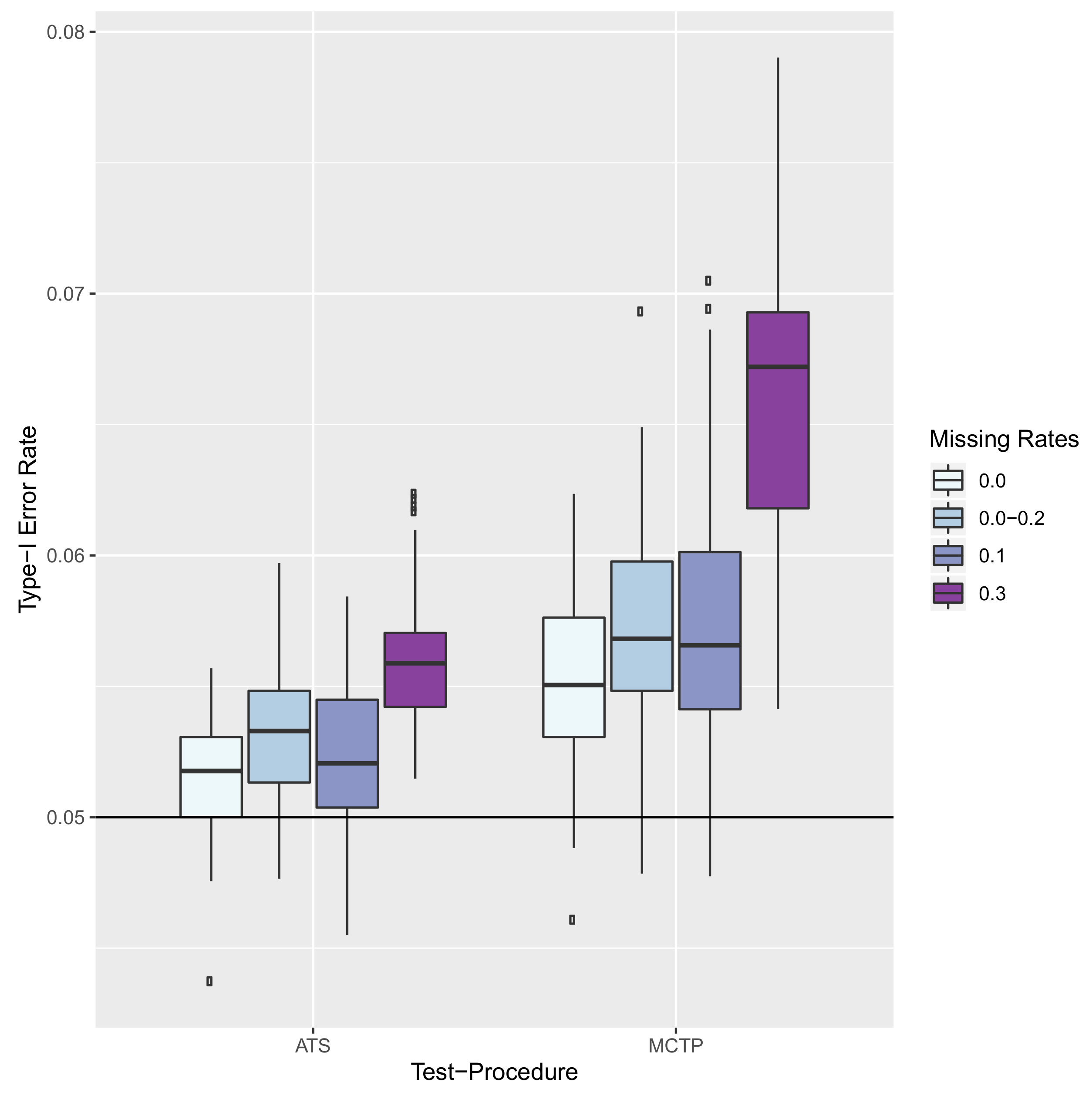
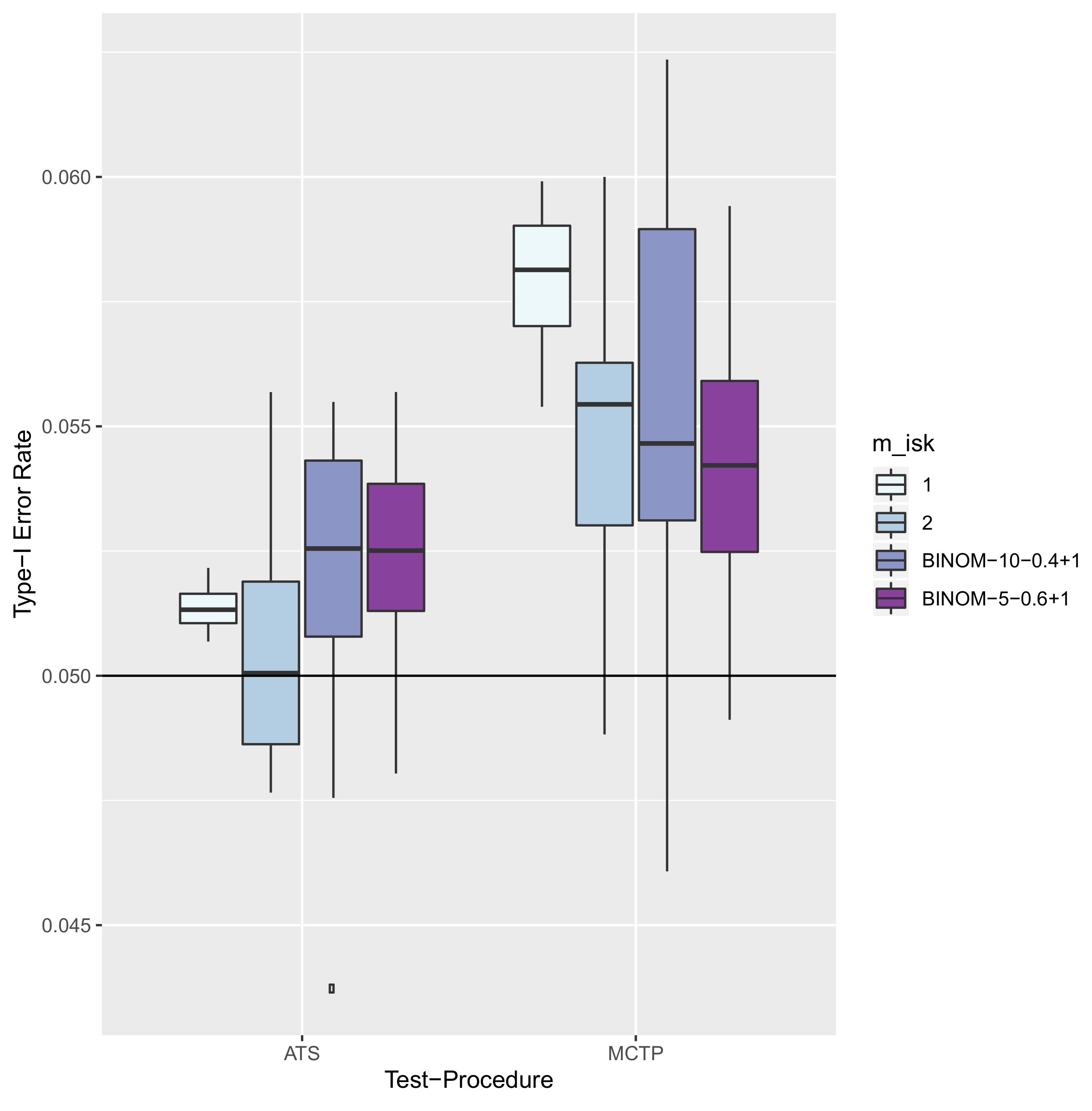
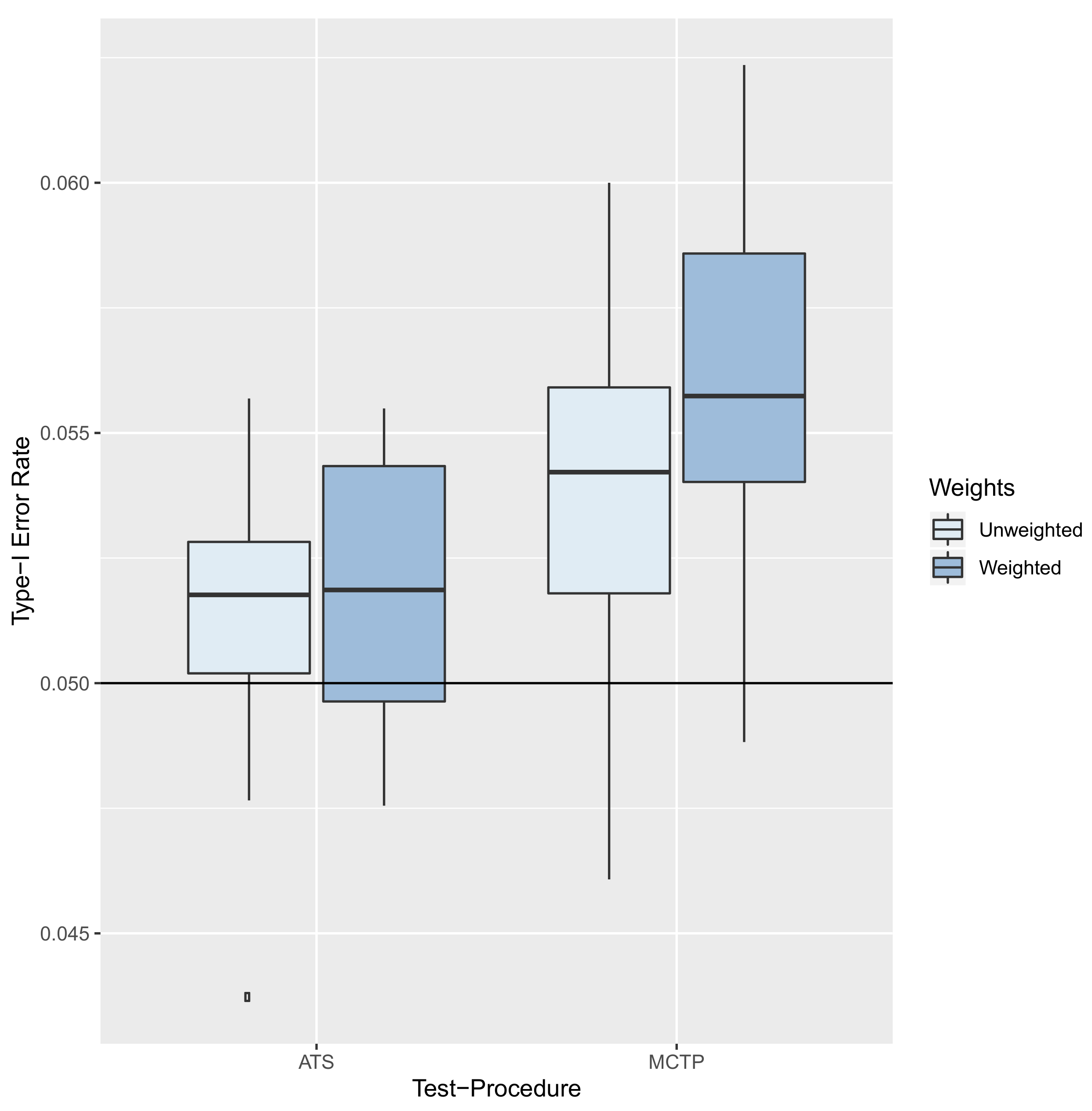
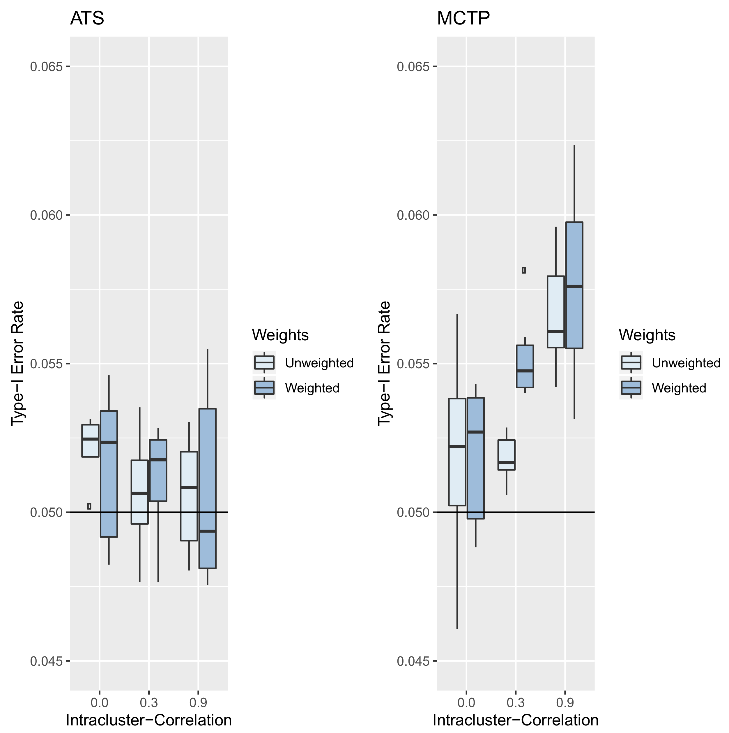
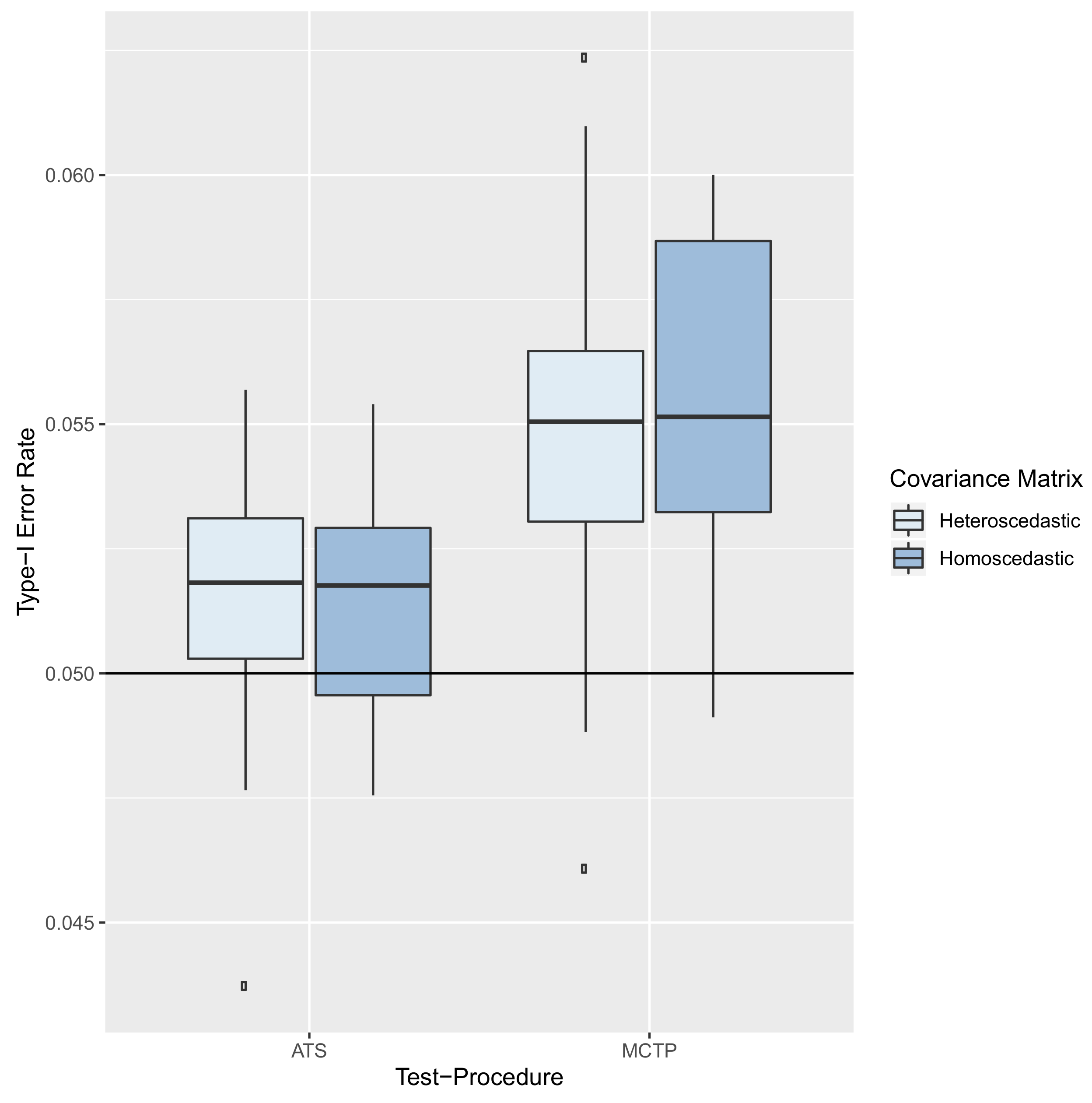
8.2. Results—Type-I Error Rate

First, an overview of the impact of different sample sizes in scenarios with completely observed data is given in Figure 1 if no missing values occur. It can be readily seen that both procedures control the type-I error quite well even if the sample size is quite low with $n_1=n_2=15$. Interestingly, the MCTP works better if sample sizes are unbalanced, whereas the ATS works better in case of balanced sample sizes.

Next, the impact of missing values will be inspected. In Figure 2, the sample sizes were fixed with $n_1=n_2=30$. The empirical type-I error rates of both procedures increase, if missing values occur and the higher the relative frequency of missing values, the higher the type-I error rates. Furthermore, the simulation study indicates that the MCTP is more affected by the occurrence of missing values than the ATS, which was already noted by Rubarth et al. [31].

The relationship between the cluster sizes $m_{isk}$ and the type-I error rates is depicted in Figure 3. For this comparison, the sample sizes were again fixed with $n_1=n_2=30$ and only completely observed data were investigated. It can be readily seen that type-I error rates decrease if two dependent replicates of each subject are present in comparison to a dataset without a clustered structure. However, type-I error rates of the ATS increases if the number of dependent replicates $m_{isk}$ is arbitrary with an expected number of dependent replicates of 5 or 4, respectively. In contrast, the type-I error rates of the MCTP decrease on median in these scenarios.

Next, the influence of intra-cluster correlations ${\rho }_{isk}$ on type-I error rates is investigated in scenarios with sample sizes $n_1=n_2=30$ and green without missing data (Figure 4). The type-I error rates of the ATS decrease if non-arbitrary higher intra-cluster correlations are present, whereas the type-I error rates of the MCTP increase in case of higher (non-arbitrary) intra-cluster correlations ${\rho }_{isk}$. Interestingly, if arbitrary correlations ${\rho }_{isk}$ are present with a mean correlation of 0.6, the type-I error rates of the ATS increase in comparison to scenarios with fixed correlations, whereas the type-I error rates of the MCTP are on the same level as in scenarios with a fixed correlation ${\rho }_{isk}=0.9$.

Figure 5 depicts the impact of homo- and heteroscedastic covariance matrices ${\mathbf{\Sigma }}_1$ and ${\mathbf{\Sigma }}_2$ in settings with $n_1=n_2=30$ and green without missing data. Again, it can be seen that the type-I error rates of the ATS are on median smaller than those of the MCTP for both homo- and heteroscedastic covariance matrices. Type-I error rates of the ATS seem to be a bit smaller in case of homoscedasticity, whereas type-I error rates of the MCTP seem to be slightly larger in homoscedastic scenarios.

Next, the relationship of unweighted and weighted estimation and type-I error rates will be inspected in scenarios with $n_1=n_2=30$ and without missing data (Figure 6). It can be readily seen that the type-I error rates of the ATS do not differ on median in case of weighted and unweighted estimation of the relative effect $\mathit{p}$, only the interquartile range is increased in case of weighted estimation. Contrary, the type-I error rates of the MCTP are on median smaller in case of unweighted estimation of the relative effect $\mathit{p}$ but without an enlargement of the respective interquartile range.

To conclude, an analysis of the impact of unweighted and weighted estimation of the relative effect $\mathit{p}$ and the fixed intracluster correlation${\rho }_{isk}$ is presented in Figure 7 (in scenarios with $n_1=n_2=30$ and without missing data). The type-I error rates of the ATS decrease if the intra-cluster correlations ${\rho }_{isk}$ increase, as already depicted in Figure 4. Interestingly, the medians of the type-I error rates are comparable in case of unweighted and weighted estimation if no intra-cluster correlation is present. However, in these scenarios, the interquartile range of the type-I error rates in case of weighted estimation is very enlarged in comparison to the case of unweighted estimation. If a medium intra-correlation is present, type-I error rates of the unweighted estimator are on median smaller than those of the weighted estimator. Here, the interquartile ranges are quite comparable. In scenarios with high intra-class correlations, the weighted estimator yields smaller type-I error rates on median; as well as a larger interquartile range.

Again, as already outlined in Figure 4, type-I error rates of the MCTP increase with higher intra-cluster correlations. The type-I error rates of the unweighted and weighted estimator are quite comparable if no intracluster-correlation is present. However, they are quite different if a medium correlation is present: type-I error rates by using the unweighted estimator tend to be smaller on median than those obtained from weighted estimation. If high correlations are present, the unweighted estimator yields smaller type-I error rates than the weighted version.

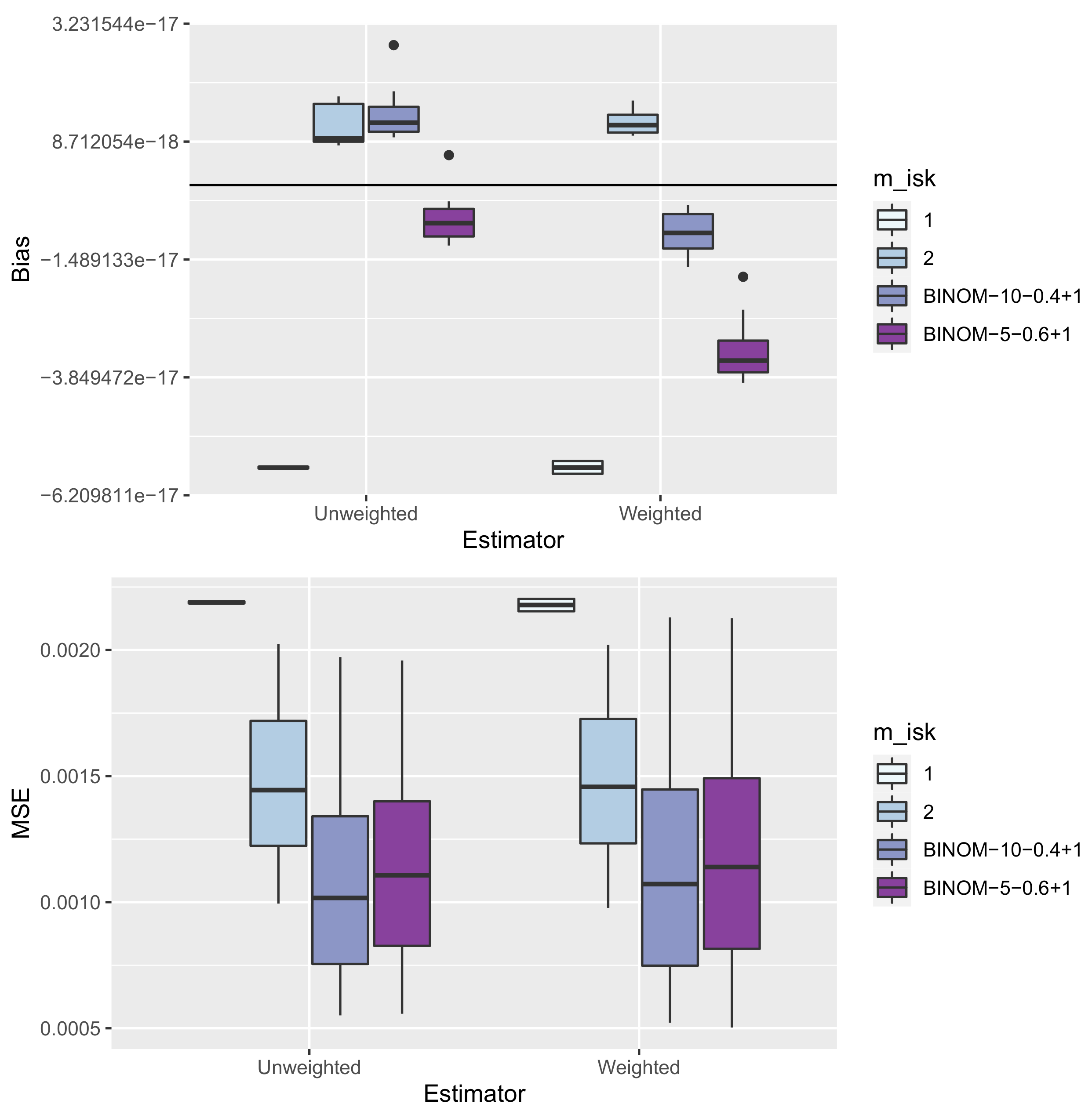
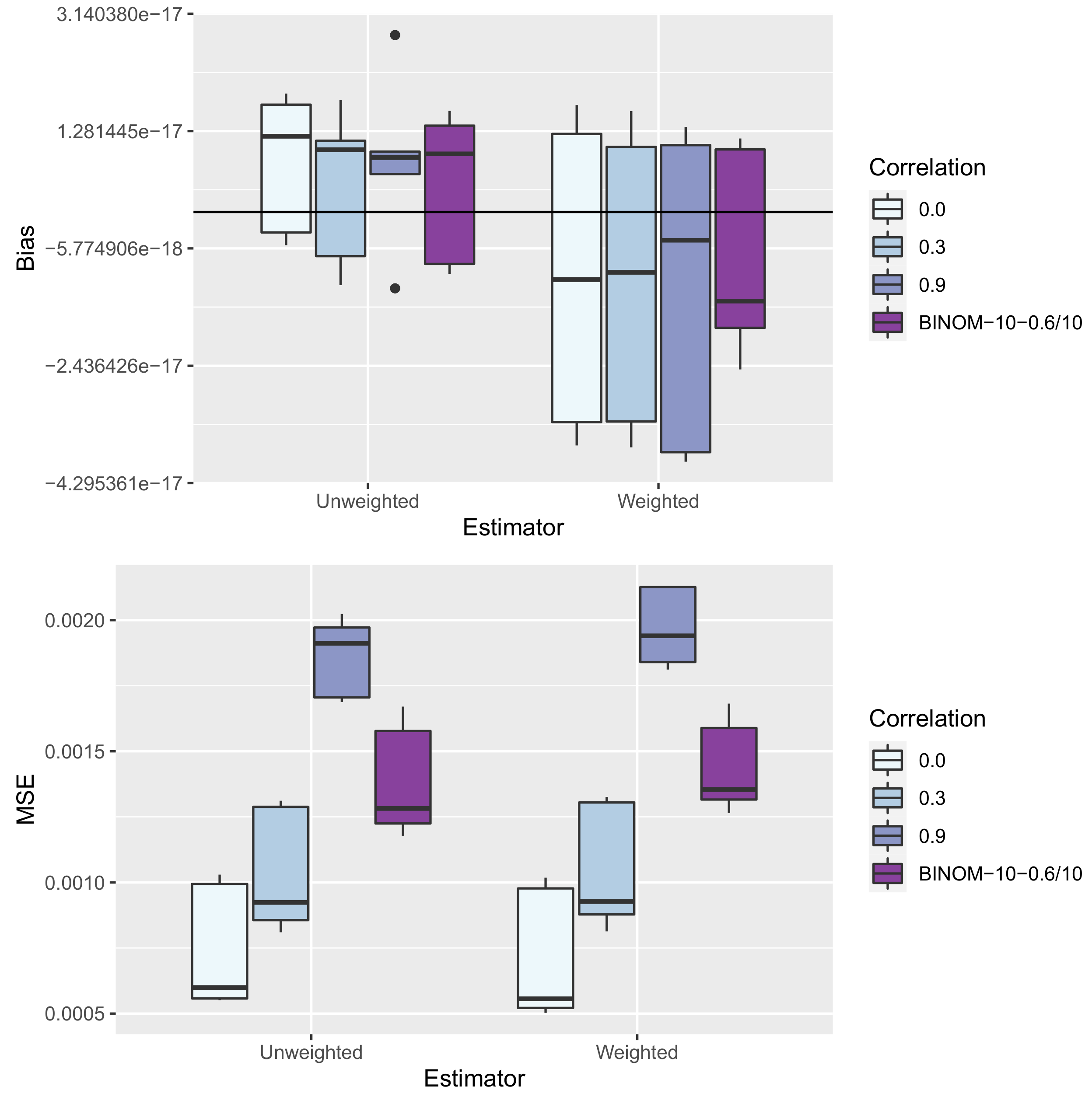
8.3. Results—Precision

Analogously to the previous section, we will first explore the impact of the sample size on the precision of the unweighted and weighted estimators in scenarios with completely observed data. It can be readily seen in Figure 8 that the MSEs of the unweighted and weighted estimators are quite comparable. The MSEs decrease if sample size increase; balanced settings exhibit smaller MSEs than unbalanced settings. Regarding the bias of the estimators, scenarios with smaller sample sizes tend to exhibit biases in the negative direction, whereas scenarios with larger sample sizes exhibit biases in the positive direction. Interestingly, the interquartile range of biases is quite enlarged in scenarios with $n_1=40$ and $n_2=20$.

Next, the impact of missing data on the precision of the estimators is inspected in scenarios with $n_1=n_2=30$ (see Figure 9). As seen before, the MSEs of unweighted and weighted estimators are quite comparable. The MSEs increase with an increasing missing rate. Interestingly, the interquartile ranges of the biases of the two different estimators are quite different; the weighted estimator exhibits a larger interquartile range (especially if 10% of data are missing) than the unweighted estimator. Further, biases of the unweighted estimator tend to be positive (except if the missing rate is 30%). Contrary, the biases of the weighted estimator tend to be negative.

In Figure 10, the influence of the number of dependent replicates $m_{isk}$ on the precision is presented (again in scenarios with $n_1=n_2=30$ and without missing data). As already pointed out, the distribution of MSEs of the unweighted and weighted estimator is very similar. Interestingly, there is very little variation if only one observation per subject and time point is available compared to scenarios with more possibly dependent replicates. Further, the MSEs decrease quite a lot if already two possibly dependent observations are available and the more clustered data are available, the smaller are the MSEs. The same observations can be made regarding the biases of both estimators.

Finally, the relationship between intra-cluster correlations will be inspected (see Figure 11, again scenarios with $n_1=n_2=30$ and without missing data). Again, the MSEs of the unweighted and the weighted estimator do not differ much. It can be readily seen that in scenarios with fixed cluster correlations, the MSEs increase with increased intra-cluster correlations. Contrary, the biases of both estimators approach 0 with increasing fixed intra-cluster correlations but the two estimators exhibit a different behavior: the biases of the unweighted estimator tend to be positive whereas the biases of the weighted estimator tend to be negative.

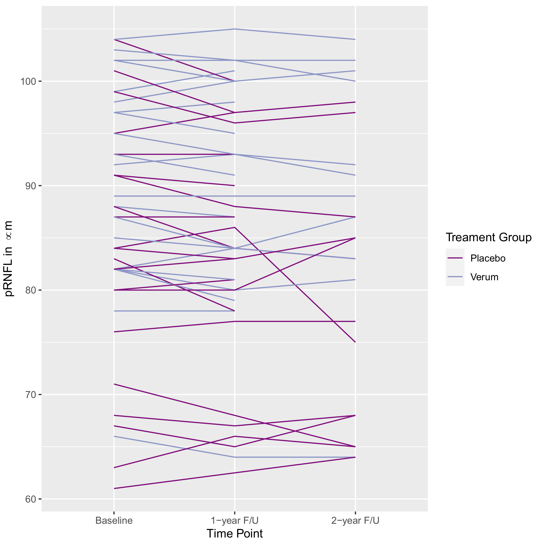
9. Analysis of the Motivating Example

The parameter pRNFL from the SUPREMES study introduced in Section 2 can now be analyzed using the newly proposed methodology for factorial repeated measures designs with dependent replicates. It can be readily seen in Figure 12 and Figure 13 that pRNFL baseline values in the placebo group tend to be smaller than those from the EGCG group.

Further, Figure 13 indicates that pRNFL values seem to increase at 2-year follow-up; however, this needs to be interpreted with caution, since almost 50% of the patients could not be measured at this time point. These were mostly patients with smaller baseline pRNFL values. This could possibly violate the Missing Completely at Random (MCAR) assumption. However, the simulation study of Rubarth et al. [31] indicated that the proposed method is robust against violations of the MCAR assumption. In order to account for the baseline differences between the two groups following Klumbies et al. [19], the analysis is not based on raw pRNFL values but on differences to baseline. In contrast to the analysis of Klumbies et al. [19], the MCTP on baseline differences is applied. The Tukey contrast was chosen to compare all pairwise differences, thus, the contrast matrix for testing the null hypothesis $H_0^p:\mathit{C}\mathit{p}=\mathbf{0}$ is as follows:

$$\mathit{C}=\left(\begin{array}{c}{\mathit{c}}_1^{\prime }\\ {\mathbf{c}}_2^{\prime }\\ {\mathit{c}}_3^{\prime }\\ {\mathit{c}}_4^{\prime }\\ {\mathit{c}}_5^{\prime }\\ {\mathit{c}}_6^{\prime }\end{array}\right)=\left(\begin{array}{cccc}-1& 1& 0& 0\\ -1& 0& 1& 0\\ -1& 0& 0& 1\\ 0& -1& 1& 0\\ 0& -1& 0& 1\\ 0& 0& -1& 1\end{array}\right).$$

The relative effects were estimated by using the unweighted version of the estimator, leading to $\widehat{\mathit{p}}={\left({\widehat{p}}_{11},{\widehat{p}}_{12},{\widehat{p}}_{21},{\widehat{p}}_{22}\right)}^{\prime }={\left(0.525,0.445,0.505,0.525\right)}^{\prime }$, indicating that the differences to baseline are the largest at 1-year follow-up simultaneously in group 1 (intervention group) and group 2 (Placebo group) and the smallest at 2-year follow-up in group 1. The results, including the values of the test statistics $T_{\ell }$, p-values and 95% simultaneous confidence intervals, are displayed in

Table 2. Point estimators of differences $p_{is}-p_{jt}$ ($i,j$: group, $s,t$: time point), simultaneous confidence intervals, t-values and p-values for Tukey-type contrasts in relative effects in the SUPREMES trial.

Comparison	Estimator	95%-Confidence Interval	t-Value	p-Value
${\widehat{p}}_{12}-{\widehat{p}}_{11}$	−0.080	[−0.371, 0.212]	−0.777	0.850
${\widehat{p}}_{21}-{\widehat{p}}_{11}$	−0.020	[−0.344, 0.303]	−0.178	0.998
${\widehat{p}}_{22}-{\widehat{p}}_{11}$	0.000	[−0.468, 0.468]	0.000	1.000
${\widehat{p}}_{21}-{\widehat{p}}_{12}$	0.059	[−0.335, 0.453]	0.429	0.969
${\widehat{p}}_{22}-{\widehat{p}}_{12}$	0.080	[−0.442, 0.601]	0.435	0.968
${\widehat{p}}_{22}-{\widehat{p}}_{21}$	0.020	[−0.306, 0.346]	0.177	0.998

.

Note that no adjustment for multiplicity was necessary, since the same critical value obtained from the MCTP was used for each comparison. It follows that no evidence exists to reject the global null hypothesis $H_0^p:\mathit{C}\mathit{p}=\mathbf{0}$, resulting in the same conclusion as already pointed out by Klumbies et al. [19]: Retinal thickness analysis did not reveal neuroprotective effects of EGCG, especially when considering the contrasts ${\widehat{p}}_{21}-{\widehat{p}}_{11}=0$ and ${\widehat{p}}_{22}-{\widehat{p}}_{12}=0$, which allow a direct comparison of the differences to baseline at 1-year and 2-year follow-up in the two groups.

10. Discussion and Conclusions

In the present paper, we presented different estimation techniques for Wilcoxon–Mann–Whitney effects in factorial repeated measures designs with clustered data. In a first step, the information whether cluster sizes are informative or non-informative is key and plays a major role in precise effect size estimation. Furthermore, as indicated by Zou [28] the use of the intraclass correlation enlarges the precision of the estimators. Anyway, besides estimation, we furthermore discussed how to test global and multiple hypotheses in terms of Wilcoxon–Mann–Whitney effects using any of the aforementioned estimators. Here, no specific data distribution (symmetric or asymmetric) is required. The presented estimators and test procedures should be preferred over standard parametric methods such as Linear Mixed Models or Generalized Estimating Equations in scenarios with small sample sizes, heteroscedastic variances or count, ordinal outcomes. We recommend to use the MCTP instead of quadratic-type test procedures in most practical applications since testing global hypotheses does not usually answer the research questions. However, the MCTP presented in this paper does not precisely hold the nominal type-I error rate in case of very small sample sizes, high correlations, and strong heteroscedasticity between groups or time points. Recently, Friedrich et al. [39] proposed novel resampling methods in purely non-parametric designs. Extending these ideas to such designs will be part of future research to improve especially the MCTP in “extreme“ scenarios.

Although an extensive simulation study was conducted to evaluate the precision and type-I error rates of the procedures in several scenarios, it is advised to conduct further simulation studies in practical applications, e.g., in the planning or data analysis phase of a study for a specific scenario. Further examinations indicate that the methods are applicable even in situations with rather small sample sizes, such as $n=10$. The actual nominal level and accuracy depends, however, on the design of interest.

Furthermore, it is important to note that many scientists in applied research fields, e.g., biomedicine, have a misconception that the Wilcoxon–Mann–Whitney (WMW) test is a test for equality of means or medians, when outcomes are metric and distributions are skewed or ordinal and that this test is the non-parametric equivalent to a classic two-sample t-test [40]. As investigated by Fagerland et al. [41], the true significance level of the WMW test deviates enormously from the nominal level when the test is used for comparing means or medians in scenarios with deviations from a pure shift model (two populations having equal shapes and scales). In practical applications, the pure shift model is rarely present, since skewed distributions with different means have most likely also different variances. Especially in such scenarios, the Brunner–Munzel test [8] should be applied. Another disadvantage of the application of WMW tests as noted by Bergmann et al. [42] is that many versions and implementations in statistical software packages exist, e.g., large sample approximation, exact permutation form, versions with or without correction for continuity or ties and different algorithm variants, all leading to possibly different p-values and eventually to different conclusions. In this work we present a unified approach that does not need a correction for ties nor continuity. Furthermore, the WMW test and its p-value are rarely accompanied with their corresponding effect estimate, the Wilcoxon–Mann–Whitney parameter p and its corresponding confidence interval. As noted by Fay et al. [43], classic confidence interval procedures for the WMW parameter are not compatible with exact WMW tests, meaning, that the tests rejects a hypothesis at significance level $\alpha$ but the confidence interval for p includes $\frac{1}{2}$. Thus, Fay et al. [43] developed compatible confidence intervals for asymptotic WMW tests and for some exact WMW tests. Furthermore, Fay et al. [44] indicate that the WMW parameter p can be framed as a causal parameter (the probability that a randomly chosen subject from one population, e.g., the treatment group in a randomized-controlled trial, will have a larger response than one subject from the other population, e.g., the control group). However, this parameter is not equal to another closely related and non-identifiable causal effect, the probability that a randomly chosen subject will have a larger response under treatment than under control [44]. This paradox was first introduced by Hand et al. [45]. Therefore, caution must be given when interpreting effect estimates from non-parametric procedures. Thus, the literacy of non-parametric statistics of scientists working in applied fields should be fostered. This work aims to accomplish this by first introducing and explaining Wilcoxon–Mann–Whitney parameters p in special designs and then providing a flexible model for the analysis of factorial repeated measure designs with a clustered structure, allowing for missing values in a second step. For user friendly applications of the methods, it is planned to enrich the R software package nparLD [46].

References

1. Roy, A.; Harrar, S.W.; Konietschke, F. The nonparametric Behrens-Fisher problem with dependent replicates. Stat. Med. 2019, 38, 4939–4962. [Google Scholar] [CrossRef] [PubMed]
2. Larocque, D.; Haataja, R.; Nevalainen, J.; Oja, H. Two sample tests for the nonparametric Behrens–Fisher problem with clustered data. J. Nonparametric Stat. 2010, 22, 755–771. [Google Scholar] [CrossRef]
3. Cui, Y.; Konietschke, F.; Harrar, S.W. The nonparametric Behrens–Fisher problem in partially complete clustered data. Biom. J. 2021, 63, 148–167. [Google Scholar] [CrossRef] [PubMed]
4. Gao, X. A Nonparametric Procedure for the Two-Factor Mixed Model with Missing Data. Biom. J. 2007, 49, 774–788. [Google Scholar] [CrossRef] [PubMed]
5. Fitzmaurice, G.; Laird, N.; Ware, J. Applied Longitudinal Analysis; John Wiley & Sons: Hoboken, NJ, USA, 2012. [Google Scholar]
6. Johnson, R.A.; Wichern, D. Applied Multivariate Statistical Analysis; Pearson Education Limited: London, UK, 2007. [Google Scholar]
7. Mann, H.B.; Whitney, D.R. On a Test of Whether one of Two Random Variables is Stochastically Larger than the Other. Ann. Math. Stat. 1947, 18, 50–60. [Google Scholar] [CrossRef]
8. Brunner, E.; Munzel, U. The Nonparametric Behrens-Fisher Problem: Asymptotic Theory and a Small-Sample Approximation. Biom. J. 2000, 42, 17–25. [Google Scholar] [CrossRef]
9. Thas, O.; Neve, J.D.; Clement, L.; Ottoy, J.P. Probabilistic index models. J. R. Stat. Soc. Ser. B 2012, 74, 623–671. [Google Scholar] [CrossRef] [Green Version]
10. Acion, L.; Peterson, J.J.; Temple, S.; Arndt, S. Probabilistic index: An intuitive non-parametric approach to measuring the size of treatment effects. Stat. Med. 2006, 25, 591–602. [Google Scholar] [CrossRef]
11. Brunner, E.; Bathke, A.C.; Konietschke, F. Rank and Pseudo-Rank Procedures for Independent Observations in Factorial Designs; Springer: Berlin/Heidelberg, Germany, 2018. [Google Scholar]
12. Akritas, M.; Kuha, J.; Osgood, W. A Nonparametric Approach to Matched Pairs with Missing Data. Sociol. Methods Res. 2002, 30, 425–454. [Google Scholar] [CrossRef]
13. Fong, Y.; Huang, Y.; Lemos, M.; Mcelrath, J. Rank-based two-sample tests for paired data with missing values. Biostatistics 2018, 19, 281–294. [Google Scholar] [CrossRef]
14. Domhof, S.; Brunner, E.; Osgood, W. Rank Procedures for Repeated Measures with Missing Values. Sociol. Methods Res. 2002, 30, 367–393. [Google Scholar] [CrossRef]
15. Amro, L.; Konietschke, F.; Pauly, M. Incompletely observed nonparametric factorial designs with repeated measurements: A wild bootstrap approach. arXiv 2021, arXiv:2102.02871. [Google Scholar]
16. Akritas, M.; Brunner, E. A unified approach to rank tests for mixed models. J. Stat. Plan. Inference 1997, 61, 249–277. [Google Scholar] [CrossRef]
17. Brunner, E.; Munzel, U.; Puri, M.L. Rank-Score Tests in Factorial Designs with Repeated Measures. J. Multivar. Anal. 1999, 70, 286–317. [Google Scholar] [CrossRef] [Green Version]
18. Brunner, E.; Domhof, S.; Langer, F. Nonparametric Analysis of Longitudinal Data in Factorial Experiments; Wiley-Interscience: Hoboken, NJ, USA, 2002; Volume 373. [Google Scholar]
19. Klumbies, K.; Rust, R.; Dörr, J.; Konietschke, F.; Paul, F.; Bellmann-Strobl, J.; Brandt, A.; Zimmermann, H.G. Retinal Thickness Analysis in Progressive Multiple Sclerosis Patients Treated With Epigallocatechin Gallate: Optical Coherence Tomography Results From the SUPREMES Study. Front. Neurol. 2021, 12, 615790. [Google Scholar] [CrossRef]
20. Walton, C.; King, R.; Rechtman, L.; Kaye, W.; Leray, E.; Marrie, R.A.; Robertson, N.; Rocca, N.L.; Uitdehaag, B.; van der Mei, I.; et al. Rising prevalence of multiple sclerosis worldwide: Insights from the Atlas of MS, third edition. Mult. Scler. J. 2020, 26, 1816–1821. [Google Scholar] [CrossRef]
21. Reich, D.S.; Lucchinetti, C.F.; Calabresi, P.A. Multiple Sclerosis. N. Engl. J. Med. 2018, 378, 169–180. [Google Scholar] [CrossRef]
22. Petzold, A.; Balcer, L.J.; Calabresi, P.A.; Costello, F.; Frohman, T.C.; Frohman, E.M.; Martinez-Lapiscina, E.H.; Green, A.J.; Kardon, R.; Outteryck, O.; et al. Retinal layer segmentation in multiple sclerosis: A systematic review and meta-analysis. Lancet Neurol. 2017, 16, 797–812. [Google Scholar] [CrossRef] [Green Version]
23. Oertel, F.C.; Zimmermann, H.G.; Brandt, A.U.; Paul, F. Optical coherence tomography in neuromyelitis optica spectrum disorders: Potential advantages for individualized monitoring of progression and therapy. Expert Rev. Neurother. 2019, 19, 31–43. [Google Scholar] [CrossRef]
24. Ruymgaart, F. A Unified Approach to the Asymptotic Distribution Theory of Certain Midrank Statistics; Springer: Berlin/Heidelberg, Germany, 2006; Volume 821, pp. 1–18. [Google Scholar]
25. Brunner, E.; Konietschke, F.; Pauly, M.; Puri, M. Rank-Based Procedures in Factorial Designs: Hypotheses about Nonparametric Treatment Effects. J. R. Stat. Soc. Ser. B 2016, 79, 1463–1485. [Google Scholar] [CrossRef] [Green Version]
26. Brunner, E.; Konietschke, F.; Bathke, A.C.; Pauly, M. Ranks and Pseudo-ranks—Surprising Results of Certain Rank Tests in Unbalanced Designs. Int. Stat. Rev. 2020, 89, 349–366. [Google Scholar] [CrossRef]
27. Obuchowski, N.A. Nonparametric analysis of clustered ROC curve data. Biometrics 1997, 53, 567–578. [Google Scholar] [CrossRef]
28. Zou, G. Confidence interval estimation for treatment effects in cluster randomization trials based on ranks. Stat. Med. 2021, 40, 3227–3250. [Google Scholar] [CrossRef]
29. Hoffman, E.; Sen, P.; Weinberg, C. Within-Cluster Resampling. Biometrika 2001, 88, 1121–1134. [Google Scholar] [CrossRef] [Green Version]
30. Williamson, J.; Datta, S.; Satten, G. Marginal Analyses of Clustered Data When Cluster Size Is Informative. Biometrics 2003, 59, 36–42. [Google Scholar] [CrossRef]
31. Rubarth, K.; Pauly, M.; Konietschke, F. Ranking Procedures for Repeated Measures Designs with Missing Data: Estimation, Testing and Asymptotic Theory. Stat. Methods Med. Res. 2022, 31, 105–118. [Google Scholar] [CrossRef] [PubMed]
32. Konietschke, F.; Hothorn, L.; Brunner, E. Rank-based multiple test procedures and simultaneous confidence intervals. Electron. J. Stat. 2012, 6, 738–759. [Google Scholar] [CrossRef] [Green Version]
33. Konietschke, F.; Bathke, A.; Hothorn, L.; Brunner, E. Testing and estimation of purely nonparametric effects in repeated measures designs. Comput. Stat. Data Anal. 2010, 54, 1895–1905. [Google Scholar] [CrossRef]
34. Akritas, M.; Arnold, S.; Brunner, E. Nonparametric Hypotheses and Rank Statistics for Unbalanced Factorial Designs. J. Am. Stat. Assoc. 1997, 92, 258–265. [Google Scholar] [CrossRef]
35. Bretz, F.; Genz, A.; Hothorn, L. On the Numerical Availability of Multiple Comparison Procedures. Biom. J. 2001, 43, 645–656. [Google Scholar] [CrossRef]
36. Konietschke, F.; Harrar, S.W.; Lange, K.; Brunner, E. Ranking procedures for matched pairs with missing data—Asymptotic theory and a small sample approximation. Comput. Stat. Data Anal. 2012, 56, 1090–1102. [Google Scholar] [CrossRef]
37. Gao, X.; Alvo, M.; Chen, J.; Li, G. Nonparametric multiple comparison procedures for unbalanced one-way factorial designs. J. Stat. Plan. Inference 2008, 138, 2574–2591. [Google Scholar] [CrossRef]
38. R Core Team. R: A Language and Environment for Statistical Computing; R Foundation for Statistical Computing: Vienna, Austria, 2013. [Google Scholar]
39. Friedrich, S.; Konietschke, F.; Pauly, M. A wild bootstrap approach for nonparametric repeated measurements. Comput. Stat. Data Anal. 2017, 113, 38–52. [Google Scholar] [CrossRef]
40. Fay, M.P.; Proschan, M.A. Wilcoxon-Mann-Whitney or t-test? On assumptions for hypothesis tests and multiple interpretations of decision rules. Stat. Surv. 2010, 4, 1–39. [Google Scholar] [CrossRef]
41. Fagerland, M.W.; Sandvik, L. The Wilcoxon–Mann–Whitney test under scrutiny. Stat. Med. 2009, 28, 1487–1497. [Google Scholar] [CrossRef]
42. Bergmann, R.; Ludbrook, J.; Spooren, W.P.J.M. Different Outcomes of the Wilcoxon-Mann-Whitney Test from Different Statistics Packages. Am. Stat. 2000, 54, 72–77. [Google Scholar]
43. Fay, M.; Malinovsky, Y. Confidence intervals of the Mann-Whitney parameter that are compatible with the Wilcoxon-Mann-Whitney test: Confidence Intervals on the Mann-Whitney Parameter. Stat. Med. 2018, 37, 3991–4006. [Google Scholar] [CrossRef]
44. Fay, M.; Brittain, E.; Shih, J.; Follmann, D.; Gabriel, E. Causal estimands and confidence intervals associated with Wilcoxon-Mann-Whitney tests in randomized experiments. Stat. Med. 2017, 37, 2923–2937. [Google Scholar] [CrossRef]
45. Hand, D.J. On Comparing Two Treatments. Am. Stat. 1992, 46, 190–192. [Google Scholar] [CrossRef]
46. Noguchi, K.; Gel, Y.R.; Brunner, E.; Konietschke, F. nparLD: An R software package for the nonparametric analysis of longitudinal data in factorial experiments. J. Stat. Softw. 2012, 50, 12. [Google Scholar] [CrossRef] [Green Version]
47. Domhof, S. Nichtparametrische Relative Effekte. Ph.D. Thesis, Niedersächsische Staats-und Universitätsbibliothek Göttingen, Göttingen, Germany, 2001. [Google Scholar]
Figure 1. Boxplots of Type-I error rates in relation to sample sizes n 1 and n 2 in various settings without missing data.
Symmetry 14 00244 g001
Figure 2. Boxplots of Type-I error rates in relation to missing rates r 1 and r 2 in various settings with n 1 = n 2 = 30 .
Symmetry 14 00244 g002
Figure 3. Boxplots of Type-I error rates in relation to cluster sizes m i s k in various settings with n 1 = n 2 = 30 and green without missing data.
Symmetry 14 00244 g003
Figure 4. Boxplots of Type-I error rates in relation to intra-cluster correlation ρ i s k in various settings with n 1 = n 2 = 30 and green without missing data.
Symmetry 14 00244 g004
Figure 5. Boxplots of Type-I error rates in relation to covariance matrices Σ 1 and Σ 2 in various settings with n 1 = n 2 = 30 and without missing data.
Symmetry 14 00244 g005
Figure 6. Boxplots of Type-I error rates in relation to unweighted and weighted estimation of the relative effect p in various settings with n 1 = n 2 = 30 and without missing data.
Symmetry 14 00244 g006
Figure 7. Boxplots of Type-I error rates in relation to unweighted and weighted estimation of the relative effect p and fixed intra-cluster correlations ρ i s k in various settings with n 1 = n 2 = 30 and without missing data.
Symmetry 14 00244 g007
Figure 8. Boxplots of biases and MSEs of estimators p ^ i s * in Equation (5) in relation to different sample sizes n 1 and n 2 .
Symmetry 14 00244 g008
Figure 9. Boxplots of biases and MSEs of estimators p ^ i s * in Equation (5) in relation to the amount of missing data in scenarios with n 1 = n 2 = 30 .
Symmetry 14 00244 g009
Figure 10. Boxplots of biases and MSEs of estimators p ^ i s * in Equation (5) in relation to cluster sizes m i s k in scenarios with n 1 = n 2 = 30 and without missing data.
Symmetry 14 00244 g010
Figure 11. Boxplots of biases and MSEs of estimators p ^ i s * in Equation (5) in relation to intra-cluster correlations ρ i s k in scenarios with n 1 = n 2 = 30 and without missing data.
Symmetry 14 00244 g011
Figure 12. Lineplot of pRNFL values in both groups at baseline, 1-year follow-up and 2-year follow-up of the SUPREMES trial.
Symmetry 14 00244 g012
Figure 13. Boxplot of pRNFL values in both groups at baseline, 1-year follow-up and 2-year follow-up of the SUPREMES trial.
Symmetry 14 00244 g013