New Localized and Periodic Solutions to a Korteweg–de Vries Equation with Power Law Nonlinearity: Applications to Some Plasma Models

Abstract

Traveling wave solutions, including localized and periodic structures (e.g., solitary waves, cnoidal waves, and periodic waves), to a symmetry Korteweg–de Vries equation (KdV) with integer and rational power law nonlinearity are reported using several approaches. In the case of the localized wave solutions, i.e., solitary waves, to the evolution equation, two different methods are devoted for this purpose. In the first one, new hypotheses with Cole–Hopf transformation are employed to find general solitary wave solutions. In the second one, the ansatz method with hyperbolic sech algorithm are utilized to obtain a general solitary wave solution. The obtained solutions recover the solitary wave solutions to all one-dimensional KdV equations with a power law nonlinearity, such as the KdV equation with quadratic nonlinearity, the modified KdV (mKdV) equation with cubic nonlinearity, the super KdV equation with quartic nonlinearity, and so on. Furthermore, two different approaches with two different formulas for the Weierstrass elliptic functions (WSEFs) are adopted for deriving some general periodic wave solutions to the evolution equation. Additionally, in the form of Jacobi elliptic functions (JEFs), the cnoidal wave solutions to the KdV-, mKdV-, and SKdV equations are obtained. These results help many authors to understand the mystery of several nonlinear phenomena in different branches of sciences, such as plasma physics, fluid mechanics, nonlinear optics, Bose Einstein condensates, and so on.

1. Introduction

Mathematical modeling of most real-life problems usually yields functional equations, such as ordinary differential equations (ODEs), partial differential equations (PDEs), fractional equations, integral equations, and so on. Many nonlinear realistic physical phenomena can be described by integrodifferential equations. These equations arise in several fields of science, such as fluid dynamics, physics of plasmas, biological models, nonlinear optics, chemical kinetics, quantum mechanics, ecological systems, electricity, ocean, and sea, and many others. Ordinary and partial differential equations have both been shown as effective tools for modeling natural phenomena in different branches of science and engineering. Therefore, it is important to be familiar with all recent analytical and numerical methods for modeling any natural and physical problem and solving it [1,2,3,4,5,6]. The following Korteweg–De Vries equation (KdV) equation is one of the most famous PDEs that has gained fame during the more than 50 years since its creation due to its ability for modeling many physical and natural phenomena in various fields of science [2,7]

$${\partial }_t\phi +\alpha \phi {\partial }_x\phi +\beta {\partial }_x^3\phi =0,$$

(1)

where $\phi \equiv \phi \left(x,t\right)$ and $\alpha$ represents the coefficient of the nonlinear term, while $\beta$ refers to the coefficient of the dispersion term. The coefficients $\left(\alpha ,\beta \right)$ are the function of physical parameters related to the model under consideration. Equation (1) serves as a model for describing the evolution of long one-dimensional structures (solitary and cnoidal waves) that can propagate in the ocean, water tanks, in different plasma models, as well as in nonlinear optics [2,3]. There is a large group of fluid mechanics and plasma physicists researchers who have worked a lot on this equation and many related equations in multi-dimensional (Kadomtsev–Petviashvili (KP) equation, Zakharov–Kuznetsov (ZK) equation, etc.) to investigate the propagation of many nonlinear structures in different models of plasmas [8,9,10,11,12]. It is known that solitary waves can be created and propagated in any system if the balance between the wave dispersion and nonlinearity is fulfilled. The solitary wave are created/generated in a laboratory and observed in astrophysical plasma, such as in the Earth’s magnetosphere, the Jovian atmosphere, the auroral zone, and in many others [13,14,15]. In addition, the solitary waves have been investigated theoretically in various plasma models [16,17,18,19].

On the other side, at some critical plasma compositions, the coefficient of the nonlinear term $\alpha$ disappears, and here the balancing condition is broken down, and Equation (1) becomes not suitable/valid for describing the solitary or cnoidal waves. Consequently, a higher order nonlinearity must be considered which leads to the following modified KdV (mKdV) equation [20,21]

$${\partial }_t\phi +\alpha {\phi }^2{\partial }_x\phi +\beta {\partial }_x^3\phi =0.$$

(2)

Studying the propagation of ion acoustic waves (IAWs), such as solitary waves in different plasma models with negative ions has been extensively made both experimentally [22,23,24] and theoretically [24,25,26,27,28,29,30] by using the family of KdV equation, mostly the KdV Equation (1) and mKdV Equation (2). Recently, the mKdV/super KdV solitons at supercritical densities in a plasma having two electrons with different temperatures has been investigated [31]. The authors in [31] used the reductive perturbation technique for reducing the basic equation of the plasma model to a super mKdV with a quartic nonlinear term at supercritical densities of the plasma compositions

$${\partial }_t\phi +\alpha {\phi }^3{\partial }_x\phi +\beta {\partial }_x^3\phi =0.$$

(3)

On the other hand, if one of the plasma components is subject to Schamel/non-isothermal distribution, then the basic equations of a plasma model can be reduced to the family of the following Schamel–KdV (SKdV) equation [32,33,34,35,36]

$${\partial }_t\phi +\alpha \sqrt{\delta \phi }{\partial }_x\phi +\beta {\partial }_x^3\phi =0,$$

(4)

where $\delta =\pm 1$ depends on the distributed particles charge which $\delta =1\left(-1\right)$ for positive (negative) charged particles.

There are various analytical and numerical methods that have been devoted to solving this family of PDEs and many other nonlinear related equations, such as the inverse scattering transform method [37], Adomian method [38,39], homotopy perturbation method [40], $G^{\prime }/G$ method [41], tanh method [2,3,42], exp function method [43], variational iteration methods [44], Bäcklund and Darboux transforms [45], sn–ns expansion method [46], the Hirota’s bilinear method [47], elliptic functions expansion method [48], and many others [2]. Motivated by these studies, in this work, we consider the generalized KdV equation

$${\partial }_t\phi +\alpha {\phi }^p{\partial }_{x}u+\beta {\partial }_{xxx}\phi =0,$$

(5)

where p is any real (integer or rational) number, such that $(p+1)(p+2)\ne 0.$ Now, our main goal is to obtain some traveling wave solutions to Equation (5) for any value to “p”. At this end, several approaches can be employed for this purpose. For deriving some general exact solitary wave solutions to Equation (5), two different approaches are reported. In the first one, the ansatz method with the Cole–Hopf transformation are introduced to find a general solitary wave solution to Equation (5). In the second scheme, the ansatz method with hypotheses “sech” are used to obtain a general formula for the solitary wave solution. In the case of the periodic solutions, two different ansatz for the Weierstrass elliptic functions (WSEFs) are presented. Moreover, we use some different ansatz in the form of Jacobi elliptic functions (JEFs) to check if they will give us a general solution to Equation (5) or not. Furthermore, the solutions for some particular cases related to Equation (5) such as the KdV Equation (1), mKdV Equation (2), super mKdV Equation (3), SKdV Equation (4), and so on, are obtained.

2. Soliton Solutions

To find a general soliton solution to the evolution Equation (5), two different approaches are introduced. In the first approach, new hypotheses with Cole–Hopf transformation are employed to find solitary wave solutions. In the second one, the ansatz method is used to obtain a solitary wave solution to Equation (5).

2.1. First Approach for the Solitary Wave Solution

Let us introduce the following hypotheses:

$$\phi (x,t)=\sqrt[p]{f(x,t)}\equiv \sqrt[p]{f}.$$

(6)

Using this hypotheses in Equation (5), we have:

$$\begin{array}{cc}\hfill & \alpha p^2{f}^3{\partial }_{x}f+p^2{f}^2\left(\beta {\partial }_x^{3}f+{\partial }_{t}f\right)-3\beta pf(p-1){\partial }_{x}f{\partial }_x^{2}f\hfill \\ \hfill & +\beta (p-1)(2p-1){\left({\partial }_{x}f\right)}^3=0,\hfill \end{array}$$

(7)

To find a general solution to Equation (7), the following Cole–Hopf transformation is employed [1]

$$f=A{\partial }_{xx}log(1+exp(kx+wt+{\xi }_0)),$$

(8)

where A and w are undetermined parameters.

Inserting ansatz (8) into (7), we have

$$-\frac{A^3{k}^6(\xi -1){\xi }^3}{{(\xi +1)}^9}\left(\left(p^{2}w+k^3\beta \right)\left(1+{\xi }^2\right)+\left(\begin{array}{c}2p^{2}w+A{k}^3{p}^2\alpha -2k^3\beta \\ -6k^{3}p\beta -2k^3{p}^2\beta \end{array}\right)\xi \right)=0,$$

(9)

where $\xi =\left(kx+wt\right).$

Equating to zero the coefficients of ${\xi }^j$ and solving the obtained system of algebraic equations, we have

$$A=\frac{2\beta \left(2+3p+p^2\right)}{\alpha p^2}\&w=-\frac{\beta k^3}{p^2}.$$

(10)

Accordingly, one-soliton solution to Equation (7) is obtained as

$$\phi (x,t)={\left(\frac{k^2\beta \left(p+1\right)\left(p+2\right)}{\alpha p^2\left(1+cosh\left(kx-\frac{\beta k^3}{p^2}t\right)\right)}\right)}^{\frac{1}{p}}.$$

(11)

Solution (11) fulfills Equation (5) for all integer values to “p”. Additionally, this solution recovers the solitary wave solutions to the KdV Equation (1), mKdV Equation (2), and super mKdV Equation (3), and so on.

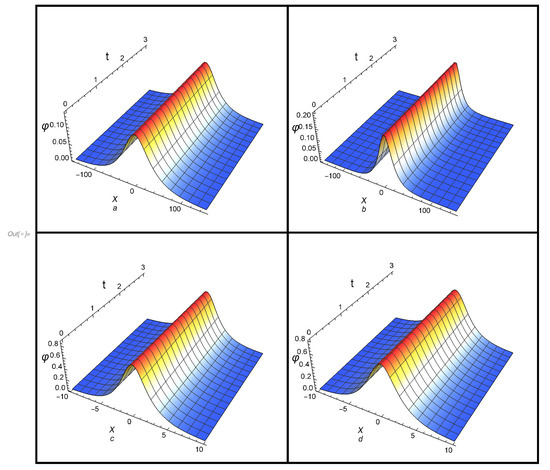
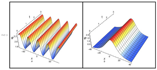
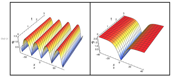
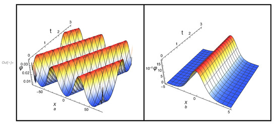
As an application to the obtained solutions, we can apply the obtained solutions for studying the behavior of solitary and cnoidal waves in different plasma models. For instance, El-Tantawy and Moslem [28] used the extended Poincaré–Lighthill–Kuo (PLK) perturbation technique for reducing the fluid equations of electron–positron–ion plasmas have non-Maxwellian electrons and positrons to two coupled KdV equations, as well as two coupled mKdV equations for investigating the solitons collisions. We can pick up some information from Ref. [28] in order to analyze our results. At certain values of the physical parameters related the plasma model in Ref. [28], the values of $\left(\alpha ,\beta \right)$ can be obtained. For the KdV Equation (1) and mKdV Equation (2) we can use ${\left(\alpha ,\beta \right)}_{\mathrm{KdV}}=\left(1.34262,0.936775\right)$ at $\left(\nu ,{\sigma }_i,{\sigma }_p,q\right)=\left(0.1,0.1,1,0.6\right)$ and ${\left(\alpha ,\beta \right)}_{\mathrm{mKdV}}=\left(0.0182189,1.65342\right)$ at $\left(\nu ,{\sigma }_i,{\sigma }_p,q\right)=\left(0.025,0.1,0.9,q_c\right)$. All papermakers mentioned here can be can be found in Ref. [28]. Moreover, we can follow the work of Verhesst et al. [31] to describe the solitary wave solution of the super KdV Equation (4). The authors reduced the fluid equations of a collisionless and unmagnetized cold plasma which consists of cold positive ions and two electrons with different temperatures that follow Maxwellian distribution, to the super KdV Equation (4) with ${\left(\alpha ,\beta \right)}_{\mathrm{Super}\mathrm{KdV}}=\left(2,1\right)$. Furthermore, for SKdV Equation (4), we can use the same data of Figure 1 in Ref. [36]: $\left(\alpha ,\beta \right)=\left(4.3,0.00285\right)$. Based on the mentioned plasma models, the profile of the solitary wave solution (11) according to $p=1$, $p=2$, and $p=3$ are presented in Figure 1a–c. Additionally, solitary wave solution for $p=4$ is considered in Figure 1d for random values to $\left(\alpha ,\beta \right)$, such as $\left(\alpha ,\beta \right)=\left(3,1\right)$. In all cases, we took $k=0.1.$

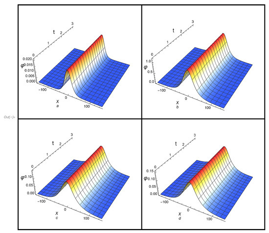
Figure 1. The profile of the solitary wave solution (11) according to $p=1$, $p=2$, $p=3$, and $p=4$ is plotted in $\left(x,t\right)-$plane.

2.2. Second Approach for the Solitary Wave Solution

Here, two hypotheses in the form of hyperbolic sech are presented.

(B-I) In this approach, the solution of Equation (5) is assumed to be

$$\left\{\begin{array}{c}\phi (x,t)=f^{\frac{2}{p}}\left(\xi \right),\\ f\left(\xi \right)=A+Bsech\left(\xi \right)\end{array}\right.$$

(12)

where $\xi =\left(kx+\lambda t+{\xi }_0\right).$

Inserting Equation (12) into Equation (5), and several simplifications the following system of algebraic equation are obtained

$$F_0=0,F_1=0,\cdots ,F_8=0,$$

(13)

where the values $F_j\left(j=0,1,\cdots ,7\right)$ are given in Appendix A and by solving system (13) in $\left(A,B,\lambda \right)$, we obtain

$$A=0,B=\pm \frac{k\sqrt{2\beta }}{p\sqrt{\alpha }}\sqrt{2+3p+p^2},\lambda =-\frac{4k^3\beta }{p^2}.$$

(14)

Substituting the values of the coefficients $\left(A,B,\lambda \right)$ given in Equation (14) into relation (12), the following soliton solution is obtained

$$\phi =2^{\frac{1}{p}}{\left(\frac{k\sqrt{\beta }\sqrt{2+3p+p^2}}{p\sqrt{\alpha }}sech\left(kx-\frac{4k^3\beta }{p^2}t\right)\right)}^{\frac{2}{p}}.$$

(15)

If the system (13) is solved in $\left(A,B,k\right)$, one obtains

$$A=0,B=\pm \frac{1}{2^{\frac{1}{6}}p\sqrt{\alpha }}\sqrt{\sqrt[3]{p^4\beta {\lambda }^2}\left(p+1\right)\left(p+2\right)},k=-\sqrt[3]{\frac{p^2\lambda }{2^2\beta }}.$$

(16)

According to the values of the coefficients $\left(A,B,k\right)$ given (16), the solitary wave solutions of Equation (5) reads

$$\phi ={\left(\pm \frac{1}{2^{\frac{1}{6}}p\sqrt{\alpha }}\sqrt{\sqrt[3]{p^4\beta {\lambda }^2}\left(p+1\right)\left(p+2\right)}sech\left(\sqrt[3]{\frac{p^2\lambda }{2^2\beta }}x-\lambda t\right)\right)}^{\frac{2}{p}}.$$

(17)

(B-II) The solution of Equation (5) can be presented in the following form

$$\left\{\begin{array}{c}\phi (x,t)=f^{\frac{2}{p}}\left(x,t\right),\\ f\left(x,t\right)=A+Bsech\left(\xi \right),\end{array}\right.$$

(18)

note here $\xi =\sqrt{k}\left(x-\lambda t\right)+{\xi }_0.$

By following the same procedure above for obtaining the solutions (15) and (17), we get:

$$A=0,B=\pm \sqrt{\frac{\lambda }{2\alpha }}\sqrt{\left(p+1\right)\left(p+2\right)},k=\frac{p^2\lambda }{4\beta }.$$

(19)

which lead to

$$\phi ={\left(\pm \sqrt{\frac{\lambda }{2\alpha }}\sqrt{\left(p+1\right)\left(p+2\right)}sech\left(\sqrt{\frac{p^2\lambda }{4\beta }}(x-\lambda t)\right)\right)}^{\frac{2}{p}}.$$

(20)

The solutions (15), (17), and (20) satisfy Equation (5) for any integer value to $p.$ Moreover, these solutions recover all solitary wave solutions to the KdV Equation (1), mKdV Equation (2), super mKdV Equation (3), and so on.

Recently, Verhesst et al. [31] derived the super mKdV Equation (3) $\left(p=3\right)$ for studying the super solitary waves in a plasma at super critical compositions. Motivated by Verheest et al. [31] investigation, the solitary wave solutions to Equation (3) according to the above relations (9), (17), and (20) are summarized in the following manner for $p=3$,

$$\begin{array}{cc}\hfill \phi & =\frac{2\times 5^{\frac{1}{3}}}{3^{\frac{2}{3}}}{\left(k\sqrt{\frac{\beta }{\alpha }}sech\left(kx-\frac{4}{9}{k}^3\beta t\right)\right)}^{\frac{2}{3}},\hfill \end{array}$$

(21)

$$\begin{array}{cc}\hfill \phi & =\frac{2^{\frac{5}{9}}\times 5^{\frac{1}{3}}}{3^{\frac{2}{9}}}{\left(\pm \sqrt{\frac{\sqrt[3]{\beta {\lambda }^2}}{\alpha }}sech\left(\sqrt[3]{\frac{9\lambda }{4\beta }}x-\lambda t\right)\right)}^{\frac{2}{3}},\hfill \end{array}$$

(22)

$$\begin{array}{cc}\hfill \phi & ={\left(\pm \sqrt{\frac{10\lambda }{\alpha }}\right)}^{\frac{2}{3}}{sech}^{\frac{2}{3}}\left(\frac{3}{2}\sqrt{\frac{\lambda }{\beta }}(x-\lambda t)\right).\hfill \end{array}$$

(23)

Note that the solutions (21)–(23) fulfill Equation (3).

The profile of the solitary wave solutions (11), (21)–(23), according to $p=3$, is graphically mapped as shown in Figure 2a–d, respectively, for $\left(\alpha ,\beta \right)=\left(2,1/2\right)$. Here, $k=0.1$ for Figure 2a,b and $\lambda =0.1$ for Figure 2c,d.

Figure 2. The profile of the solitary wave solutions (11), (21)–(23) according to $p=3$, i.e., for super mKdV Equation (3) is plotted in $\left(x,t\right)-$plane.

3. Periodic Solutions in Terms of WSEFs and JEFs

Inserting the following traveling wave transformation

$$\phi =v^{\frac{1}{p}},$$

(24)

into Equation (5), we get

$$\begin{array}{cc}\hfill & p^{2}v{\left(\xi \right)}^2\left(\beta k^3{v}^{\left(3\right)}\left(\xi \right)+\lambda v^{\prime }\left(\xi \right)\right)+\beta k^3(p-1)(2p-1)v^{\prime }{\left(\xi \right)}^3\hfill \\ \hfill & -3\beta k^3(p-1)pv\left(\xi \right)v^{\prime }\left(\xi \right)v^{″}\left(\xi \right)+\alpha k{p}^{2}v{\left(\xi \right)}^3{v}^{\prime }\left(\xi \right)=0,\hfill \end{array}$$

(25)

where $\xi =kx+\lambda t$.

Here, the main goal is to obtain some general periodic wave solutions to Equation (25). To end this, in the below sub-sections, some different formulas for the periodic wave solutions are introduced.

3.1. First Formula in Terms of WSEFs

We seek for solutions to the ODE (25) in the ansatz form

$$v\left(\xi \right)=A+B\wp (\xi +C;g_2,g_3),$$

(26)

where $\wp \equiv \wp (\xi +C;g_2,g_3)$ indicates WSEFs and $\left(g_2,g_3\right)$ are called the invariants. This function obeys the following ODE

$${\wp }^{\prime }=\sqrt{4{\wp }^3-g_2\wp -g_3},$$

(27)

Inserting the ansatz (26) into Equation (25) taking Equation (27) into account, we get

$${\wp }^{\prime }\frac{B}{2}{\displaystyle \sum _{j=0}^3}{S}_j{\wp }^j=0,$$

(28)

where the values of $S_j\left(j=0,1,2,3\right)$ are defined in the Appendix B,

Equating the coefficients $S_i$ to zero, solving the system: $S_0=0$,$\cdots ,S_3=0,$ we finally obtain the values of $\left(B,\lambda ,g_2,g_3\right)$

$$\begin{array}{cc}\hfill B& =-\frac{2\beta k^2(p+1)(p+2)}{\alpha p^2},\lambda =-\frac{6\alpha Ak}{(p+1)(p+2)},\hfill \\ \hfill g_2& =\frac{3{\alpha }^2{A}^2{p}^4}{{\beta }^2{k}^4{(p+1)}^2{(p+2)}^2},g_3=-\frac{{\alpha }^3{A}^3{p}^6}{{\beta }^3{k}^6{(p+1)}^3{(p+2)}^3}\hfill \end{array}$$

(29)

The values of the constants A, $C,$ and k can be estimated from the following initial conditions

$$v\left(0\right)=v_0,v^{\prime }\left(0\right)={\dot{v}}_0,v^{″}\left(0\right)={\ddot{v}}_0.$$

(30)

Applying the conditions (30), we obtain

$$\begin{array}{cc}\hfill A& =\frac{2v_0{\ddot{v}}_0-3{\dot{v}}_0^2}{6(v_0{\ddot{v}}_0-{\dot{v}}_0^2)}{v}_0,\hfill \\ \hfill C& ={\wp }^{-1}\left(\frac{4v_0{\ddot{v}}_0-3{\dot{v}}_0^2}{12v_0^2};\frac{\left(3{\dot{v}}_0^2-2v_0{\ddot{v}}_0\right){}^2}{12v_0^4},\frac{\left(2v_0{\ddot{v}}_0-3{\dot{v}}_0^2\right){}^3}{216v_0^6}\right),\hfill \\ \hfill k& =\frac{\sqrt{\alpha }p{v}_0^{3/2}}{\sqrt{\beta (p+1)(p+2)\left({\dot{v}}_0^2-v_0{\ddot{v}}_0\right)}}.\hfill \end{array}$$

(31)

Substituting the values of the coefficients given in Equations (29) and (31), the traveling wave solutions of the generalized third-order KdV (5) are obtained

$$\phi =\sqrt[p]{\frac{v_0}{6\left(v_0{\ddot{v}}_0-{\dot{v}}_0^2\right)}\left[\begin{array}{c}2v_0{\ddot{v}}_0-3{\dot{v}}_0^2\\ +12v_0^2\wp \left(\frac{\sqrt{\alpha }p{v}_0^{3/2}}{\sqrt{\beta (p+1)(p+2)\left({\dot{v}}_0^2-v_0{\ddot{v}}_0\right)}}x-\frac{6\alpha Ak}{(p+1)(p+2)}t+C;g_2,g_3\right)\end{array}\right]},$$

(32)

where the values of $v_0$,${\dot{v}}_0,$ and ${\ddot{v}}_0$ are arbitrary.

3.2. Second Formula in Terms of WSEFs

We proceed to obtain a solution to the ODE (25) in the ansatz form

$$v\left(\xi \right)=A+\frac{B}{1+C\wp (\xi +D;g_2,g_3)}.$$

(33)

Inserting ansatz (33) into Equation (25), we finally get

$${\displaystyle \sum _{j=0}^4}{Z}_j{w}^4=0,$$

where $w=\wp (\xi +D;g_2,g_3)$ and in the Appendix C, the values of $Z_j\left(j=0,1,\cdots ,4\right)$ are defined.

The solution of system: $Z_0=0,\cdots$, $Z_4=0,$ will give us

$$\begin{array}{cc}\hfill B& =-\frac{3A}{2},C=\frac{3\beta k^2(p+1)(p+2)}{\alpha A{p}^2},\lambda =-\frac{2\alpha Ak}{(p+1)(p+2)},\hfill \\ \hfill g_2& =\frac{{\alpha }^2{A}^2{p}^4}{3{\beta }^2{k}^4{(p+1)}^2{(p+2)}^2},g_3=-\frac{{\alpha }^3{A}^3{p}^6}{27{\beta }^3{k}^6{(p+1)}^3{(p+2)}^3}\hfill \end{array}$$

(34)

where the values of A, $k,$ and D are obtained from the initial conditions given in Equation (30).

3.3. Third Formula in Terms of JEFs

In this part, we start our analysis by an important question: does Equation (5) has a cnoidal wave solution for any value to “p”?. To check that, two hypotheses in the form of JEFs are presented.

(I) Introducing the first ansatz

$$\left\{\begin{array}{c}\phi (x,t)=f^{\frac{1}{p}}\left(x,t\right),\\ f\left(x,t\right)=A+Bc{n}^2\left(\left.\sqrt{k}(x-\lambda t)\right|m\right)\end{array}\right.$$

(35)

into Equation (5) and after several sequential arithmetic calculations, we have

$$A=0,B=\frac{\left(2+3p+p^2\right)\lambda }{2\alpha },k=\frac{p^2\lambda }{4\beta },m=1.$$

(36)

The substitution of the values $\left(A,k,m\right)$ into solution (35), give us the soliton solution

$$\phi (x,t)={\left(\frac{\left(2+3p+p^2\right)\lambda }{2\alpha }\right)}^{\frac{1}{p}}{\sec \mathrm{h}}^{\frac{2}{p}}\left(\sqrt{\frac{p^2\lambda }{4\beta }}\left(x-\lambda t\right)\right).$$

(37)

(II) Using the following second-ansatz into Equation (5)

$$\left\{\begin{array}{c}\phi (x,t)=f^{\frac{1}{p}}\left(x,t\right),\\ f\left(x,t\right)=A+\frac{B}{1+Ccn\left(\left.\sqrt{k}(x-\lambda t)\right|m\right)},\end{array}\right.$$

(38)

and after several sequential but tedious calculations, one gets

$$B=-A,C=\mp 1,\lambda =\frac{A\alpha }{\left(2+3p+p^2\right)},k=\frac{A\alpha p^2}{\beta \left(2+3p+p^2\right)},m=1,$$

(39)

where A is a non-zero arbitrary constant. From Equations (38) and (39), the solitons solutions are obtained

$$\phi (x,t)={\left(A-\frac{A}{1\pm \sec \mathrm{h}\left(\sqrt{\frac{A\alpha p^2}{\beta \left(2+3p+p^2\right)}}\left(x-\frac{A\alpha t}{\left(2+3p+p^2\right)}\right)\right)}\right)}^{\frac{1}{p}},$$

this solution satisfies Equation (5) for any integer values for $p.$

In the two cases, it is clear that the value of modulus m equals “1” which means that there is no cnoidal wave solution to the Equation (5) using the two hypotheses (35) and (38) (maybe exist cnoidal wave solution via another ansatz), but there is a cnoidal wave solution for some special cases, such as $p=1,1/2,2$. These cases will be discussed in the below sub-sections. We consider three important particular cases to $p\left(=1,2,1/2\right)$ which equivalent, the KdV Equation (1), mKdV Equation (2), and SKdV Equation (4), respectively.

4. Periodic and Localized Solutions for Some Particular Cases

4.1. Cnoidal Wave Solution to a KdV Equation

For $p=1$, Equation (5) reduces to the third order KdV Equation (1)

$${\partial }_t\phi +\alpha \phi {\partial }_x\phi +\beta {\partial }_x^3\phi =0.$$

(40)

According to the ansatz $\phi (x,t)=A+Bc{n}^2(kx-\lambda t),m)$, the cnoidal wave solutions to Equation (40) reads

$$\phi (x,t)=\frac{4\beta k^2}{\alpha }-\frac{8\beta k^{2}m}{\alpha }+\frac{\lambda }{\alpha k}+\frac{12\beta k^{2}m}{\alpha }\mathrm{cn}{\left(\left.kx-t\lambda \right|m\right)}^2,$$

(41)

and for limiting $m\to 1$, solution (41) recovers the solitary wave solution

$$\phi (x,t)=-\frac{4\beta k^2}{\alpha }+\frac{\lambda }{\alpha k}+\frac{12\beta k^2}{\alpha }{\sec \mathrm{h}}^2(kx-\lambda t).$$

(42)

Both solutions (41) and (42) satisfy Equation (54). The profiles of both cnoidal and solitary wave solutions (41) and (42) are, respectively, plotted in Figure 3a,b.

Figure 3. The profiles of both cnoidal and solitary wave solutions (41) and (42) to KdV Equation (40) are plotted in $\left(x,t\right)-$plane for $\left(\alpha ,\beta ,\lambda ,k\right)=\left(1.34262,0.936775,0.01,0.1\right)$.

4.2. Cnoidal Wave Solution to a mKdV Equation

The mKdV Equation (2) describes the critical case for vanishing the quadratic nonlinearity of the KdV Equation (1) which Equation (5) could be reduced to the mKdV Equation (2) for $p=2$ as

$${\partial }_t\phi +\alpha {\phi }^2{\partial }_x\phi +\beta {\partial }_x^3\phi =0.$$

(43)

By substituting the following ansatz into Equation (43)

$$\phi (x,t)=A+Bc{n}^2\left(\left.kx-\lambda t\right|m\right),$$

(44)

the following cases are obtained:

$$\begin{array}{cc}\hfill \mathrm{Case}\left(\mathrm{I}\right):& A=0,B=\frac{6\beta k^{2}m}{\alpha },\lambda =\beta k^3(2m-1),\hfill \end{array}$$

(45)

$$\begin{array}{cc}\hfill \mathrm{Case}\left(\mathrm{II}\right):& A=-\frac{6\beta k^2(m-1)}{\alpha },B=\frac{6\beta k^{2}m}{\alpha },\lambda =2\beta k^3-\beta k^{3}m,\hfill \end{array}$$

(46)

$$\begin{array}{cc}\hfill \mathrm{Case}\left(\mathrm{III}\right):& A=-\frac{6\beta k^{2}m}{\alpha },B=\frac{6\beta k^{2}m}{\alpha },\lambda =\beta k^3(-m)-\beta k^3,\hfill \end{array}$$

(47)

which lead to the following

For case (I), the following cnoidal and solitory ($m\to 1)$ wave solutions are obtained

$$\begin{array}{cc}\hfill \phi (x,t)& =\sqrt{\frac{6\beta k^{2}m}{\alpha }}\sqrt{\mathrm{cn}{\left(\left.kx-k^3(2m-1)t\beta \right|m\right)}^2},\hfill \end{array}$$

(48)

$$\begin{array}{cc}\hfill \phi (x,t)& =\sqrt{\frac{6\beta k^2}{\alpha }}\sqrt{{\sec \mathrm{h}}^2\left(kx-\beta k^{3}t\right)}.\hfill \end{array}$$

(49)

For case (II), the following cnoidal and solitory ($m\to 1)$ wave solutions are recovered

$$\begin{array}{cc}\hfill \phi (x,t)& =\sqrt{\frac{6\beta k^{2}m\mathrm{cn}{\left(\left.kx-t\left(2k^3\beta -k^{3}m\beta \right)\right|m\right)}^2}{\alpha }-\frac{6\beta k^2(m-1)}{\alpha }},\hfill \end{array}$$

(50)

$$\begin{array}{cc}\hfill \phi (x,t)& =\sqrt{\frac{6\beta k^2}{\alpha }}\sqrt{{\sec \mathrm{h}}^2\left(kx-\beta k^{3}t\right)}.\hfill \end{array}$$

(51)

For the case (III), we finally get the cnoidal and solitory ($m\to 1)$ wave solutions

$$\begin{array}{cc}\hfill \phi (x,t)& =\sqrt{\frac{6\beta k^{2}m\mathrm{cn}{\left(\left.kx-t\left(-m\beta k^3-\beta k^3\right)\right|m\right)}^2}{\alpha }-\frac{6\beta k^{2}m}{\alpha }},\hfill \end{array}$$

(52)

$$\begin{array}{cc}\hfill \phi (x,t)& =\sqrt{\frac{6\beta k^2{\sec \mathrm{h}}^2\left(2\beta k^{3}t+kx\right)}{\alpha }-\frac{6\beta k^2}{\alpha }}.\hfill \end{array}$$

(53)

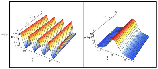
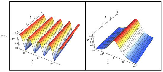
The solutions of all cases (48)–(53) satisfy Equation (43). Note that in case (III), the condition $\alpha \beta <0$ must be fulfilled. The profiles of both cnoidal and solitary waves according to the solutions of case (I): (48) and (49), case (II): (50) and (51), and case (III): (52) and (53), are, respectively, plotted in Figure 4a,b, Figure 5a,b and Figure 6a,b.

Figure 4. The profiles of both cnoidal and solitary wave solutions (48) and (49) to mKdV Equation (43) are plotted in $\left(x,t\right)-$plane for $\left(\alpha ,\beta ,k\right)=\left(0.0182189,1.65342,0.1\right)$.

Figure 5. The profiles of both cnoidal and solitary wave solutions (50) and (51) to mKdV Equation (43) are plotted in $\left(x,t\right)-$plane for $\left(\alpha ,\beta ,k\right)=\left(0.0182189,1.65342,0.1\right)$.

Figure 6. The profiles of both cnoidal and solitary wave solutions (52) and (53) to mKdV Equation (43) are plotted in $\left(x,t\right)-$plane for $\left(\alpha ,\beta ,k\right)=\left(-0.0182189,1.65342,0.1\right)$.

4.3. Cnoidal Wave Solution to a SKdV Equation

The following Schamel–KdV (SKdV) equation is obtained for $p=1/2$,

$${\partial }_t\phi +\alpha \sqrt{\delta u}{\partial }_x\phi +\beta {\partial }_{xxx}\phi =0,\delta =\pm 1.$$

(54)

Inserting the following traveling wave transformation

$$\left\{\begin{array}{c}\phi =\delta {\left(A+Bc{n}^2\left(\xi ,m\right)\right)}^2,\\ \xi =\sqrt{k}\left(x-\lambda t\right).\end{array}\right.$$

(55)

into Equation (54), the following system is obtained

$$\begin{array}{cc}\hfill -\alpha A^2\delta +4A\beta k-8A\beta km+A\lambda -6\beta Bk+6\beta Bkm& =0,\hfill \\ \hfill -2\alpha AB\delta +12A\beta km+16\beta Bk-32\beta Bkm+B\lambda & =0,\hfill \\ \hfill -B(\alpha B\delta -30\beta km)& =0.\hfill \end{array}$$

(56)

By solving system (56), we have

$$\begin{array}{cc}\hfill A& =-\frac{5}{8\alpha \delta }\left(-16k\beta +32k\beta m-\lambda \right),\hfill \\ \hfill B& =\frac{30k\beta m}{\alpha \delta },k=\frac{\lambda }{16\beta \sqrt{1+m^2-m}},\hfill \end{array}$$

which lead to

$$\phi ={\left[-\frac{5}{8\alpha }\left(-\lambda +\frac{\lambda \left(2m-1\right)}{\sqrt{1-m+m^2}}\right)+\frac{15\lambda m}{8\alpha \sqrt{1-m+m^2}}cn{\left(\frac{1}{4}\sqrt{\frac{\lambda }{\beta \sqrt{m^2-m+1}}}(x-t\lambda ),m\right)}^2\right]}^2.$$

(57)

A soliton solution is obtained for limiting $m\to 1$ as follows

$$\phi =\frac{225{\lambda }^2}{64{\alpha }^2}sech{}^4\left(\frac{1}{4}\sqrt{\frac{\lambda }{\sqrt{{\beta }^2}}}(x-\lambda t)\right).$$

(58)

Both solutions (57) and (58) satisfy Equation (54). The profiles of both cnoidal and solitary wave solutions (57) and (58) are, respectively, plotted in Figure 7a,b.

Figure 7. The profiles of both cnoidal and solitary wave solutions (57) and (58) to SKdV Equation (54) are plotted in $\left(x,t\right)-$plane for $\left(\alpha ,\beta ,\lambda \right) = \left(4.3,0.00285,0.1\right)$.

5. Conclusions

In this paper, both localized and periodic nonlinear structures solutions to a Korteweg–de Vries equation with integer and rational power law nonlinearity have been investigated analytically using several approaches. Consequently, the objectives of this paper are divided into two parts: in the first part, the general solitary wave solutions to the evolution equation using two different schemes have been obtained. In the second part, several general periodic solutions in the form of WSEFs to the evolution equation have been derived using different hypotheses. In the first, a general formula for the solitary wave solution has been obtained using the Cole–Hopf transformation. In addition, the ansatz method has been devoted to obtain another formula for the solitary solutions. It has been verified that both formulas of the solitary wave solutions for any integer and rational power law nonlinearity fulfill the evolution equation. On the other side, two different ansatz in the form of WSEFs have been presented for getting some general periodic solutions to the evolution equation. Furthermore, the solutions to some particular cases related to the evolution Equation (5) in the form of JEFs, such as the KdV Equation (1), mKdV Equation (2), Schamel KdV Equation (4), and so on, have been derived in detail. Since this family of the KdV equation has many applications in several branches of science, such as plasma physics, fluid mechanics, nonlinear optics, optical fibers, Bose Einstein condensates, etc. Therefore, the obtained solutions can help a large segment of researchers interested in the field of fluids in general, and plasma physics in particular [28,29,30,31,32,33,34,35,36,37].

References

- Wazwaz, A.M. The Cole–Hopf transformation and multiple soliton solutions for the integrable sixth-order Drinfeld–Sokolov–Satsuma–Hirota equation. Appl. Math. Comput. 2009, 207, 248. [Google Scholar] [CrossRef]
- Wazwaz, A.M. Partial Differential Equations and Solitary Waves Theory; Higher Education Press: Beijing, China, 2009. [Google Scholar]
- Wazwaz, A.M. Partial Differential Equations: Methods and Applications; Balkema, Cop.: Lisse, The Netherlands, 2002. [Google Scholar]
- Wazwaz, A.M. New (3+1)-dimensional Painlevé integrable fifth-order equation with third-order temporal dispersion. Nonlinear Dyn. 2021, 106, 891. [Google Scholar] [CrossRef]
- Kumar, V.; Wazwaz, A.M. Lie symmetry analysis for complex soliton solutions of coupled complex short pulse equation. Math. Methods Appl. Sci. 2021, 44, 5238. [Google Scholar] [CrossRef]
- Ray, S.S.; Agrawal, O.P.; Bera, R.K.; Das, S.; Raja Sekhar, T. Analytical and Numerical Methods for Solving Partial Differential Equations and Integral Equations Arising in Physical Models. Abstr. Appl. Anal. 2013, 2014, 635235. [Google Scholar] [CrossRef]
- Albalawi, W.; El-Tantawy, S.A.; Salas, A.H. On the rogue wave solution in the framework of a Korteweg–de Vries equation. Resultsin Phys. 2021, 30, 104847. [Google Scholar] [CrossRef]
- Mamun, A.A.; Eliasson, B.; Shukla, P.K. Dust-acoustic solitary and shock waves in a strongly coupled liquid state dusty plasma with a vortex-like ion distribution. Phys. Lett. A 2004, 332, 412. [Google Scholar] [CrossRef]
- Faraz, N.; Sadaf, M.; Akram, G.; Zainab, I.; Khan, Y. Effects of fractional order time derivative on the solitary wave dynamics of the generalized ZK–Burgers equation. Results Phys. 2021, 25, 104217. [Google Scholar] [CrossRef]
- El-Tantawy, S.A.; Salas, A.H.; Alharthi, M.R. Novel analytical cnoidal and solitary wave solutions of the Extended Kawahara equation. Chaos Solitons Fractals 2021, 147, 110965. [Google Scholar] [CrossRef]
- Ruderman, M.S. Freak waves in laboratory and space plasmas. Eur. Phys. J. Spec. Top. 2010, 185, 57. [Google Scholar] [CrossRef] [Green Version]
- Ruderman, M.S.; Talipova, T.; Pelinovsky, E. Dynamics of modulationally unstable ion-acoustic wavepackets in plasmas with negative ions. J. Plasma Phys. 2008, 74, 639. [Google Scholar] [CrossRef] [Green Version]
- Sharma, S.K.; Bailung, H. Observation of hole Peregrine soliton in a multicomponent plasma with critical density of negative ions. J. Geophys. Res. 2013, 118, 919–924. [Google Scholar] [CrossRef]
- Sheridan, T.E.; Nosenko, V.; Goree, J. Experimental study of nonlinear solitary waves in two-dimensional dusty plasma. Phys. Plasmas 2008, 15, 073703. [Google Scholar] [CrossRef] [Green Version]
- Bandyopadhyay, P.; Prasad, G.; Sen, A.; Kaw, P.K. Experimental Study of Nonlinear Dust Acoustic Solitary Waves in a Dusty Plasma. Phys. Rev. Lett. 2008, 101, 065006. [Google Scholar] [CrossRef] [Green Version]
- Lakhina, G.S.; Singh, S.V.; Kakad, A.P. Ion- and electron-acoustic solitons and double layers in multi-component space plasmas. Adv. Space Res. 2011, 47, 1558. [Google Scholar] [CrossRef]
- Khalid, M.; El-Tantawy, S.A.; Rahman, A.U. Oblique ion acoustic excitations in a magnetoplasma having κ-deformed Kaniadakis distributed electrons. Astrophys. Space Sci. 2020, 365, 75. [Google Scholar] [CrossRef]
- Kashkari, B.S.; El-Tantawy, S.A.; Salas, A.H.; El-Sherif, L.S. Homotopy perturbation method for studying dissipative nonplanar solitons in an electronegative complex plasma. Chaos Solitons Fractals 2020, 130, 109457. [Google Scholar] [CrossRef]
- L-Awady, E.I.E.; El-Tantawy, S.A.; Abdikian, A. Dissipative Cylindrical Magnetosonic Solitary Waves in a Magnetized quantum dusty plasma. Rom. Rep. Phys. 2019, 71, 105. [Google Scholar]
- El-Tantawy, S.A.; Wazwaz, A.M. Anatomy of modified Korteweg–de Vries equation for studying the modulated envelope structures in non-Maxwellian dusty plasmas: Freak waves and dark soliton collisions. Phys. Plasmas 2018, 25, 092105. [Google Scholar] [CrossRef]
- El-Tantawy, S.A.; Aboelenen, T.; Ismaeel, S.M.E. Local discontinuous Galerkin method for modeling the nonplanar structures (solitons and shocks) in an electronegative plasma. Phys. Plasmas 2019, 26, 022115. [Google Scholar] [CrossRef]
- Ludwig, G.O.; Ferreira, J.L.; Nakamura, Y. Observation of ionacoustic rarefaction solitons in a multicomponent plasma with negative ions. Phys. Rev. Lett. 1984, 52, 275. [Google Scholar] [CrossRef]
- Sharma, S.K.; Devi, K.; Adhikary, N.C.; Bailung, H. Transition of ion-acoustic perturbations in multicomponent plasma with negative ions. Phys. Plasmas 2008, 15, 082111. [Google Scholar] [CrossRef]
- Nakamura, Y.; Tsukabayashi, I. Observation of modified Korteweg-de Vries solitons in a multicomponent plasma with negative ions. Phys. Rev. Lett. 1984, 52, 2356. [Google Scholar] [CrossRef]
- Tagare, S.G. Effect of ion temperature on ion-acoustic soliton in a two ion warm plasma with adiabatic positive and negative ions and isothermal electrons. J. Plasma Phys. 1986, 36, 301. [Google Scholar] [CrossRef]
- Washimi, H.; Taniuti, T. Propagation of ion-acoustic solitary waves of small amplitude. Phys. Rev. Lett. 1966, 17, 996. [Google Scholar] [CrossRef]
- Watanabe, S. Ion acoustic soliton in plasma with negative ion. J. Phys. Soc. Jpn. 1984, 53, 950. [Google Scholar] [CrossRef]
- El-Tantawy, S.A.; Moslem, W.M. Nonlinear structures of the Korteweg-de Vries and modified Korteweg-de Vries equations in non-Maxwellian electron-positron-ion plasma: Solitons collision and rogue waves. Phys. Plasmas 2014, 21, 052112. [Google Scholar] [CrossRef]
- El-Tantawy, S.A. Rogue waves in electronegative space plasmas: The link between the family of the KdV equations and the nonlinear Schrödinger equation. Astrophys. Space Sci. 2016, 361, 164. [Google Scholar] [CrossRef]
- El-Tantawy, S.A. Nonlinear dynamics of soliton collisions in electronegative plasmas: The phase shifts of the planar KdV-and mkdV-soliton collisions. Chaos Solitons Fractals 2016, 93, 162. [Google Scholar] [CrossRef]
- Verheest, F.; Olivier, C.P.; Hereman, W.A. Modified Korteweg-de Vries solitons at supercritical densities in two-electron temperature plasmas. J. Plasma Phys. 2016, 82, 905820208. [Google Scholar] [CrossRef] [Green Version]
- Ghosh, S.; Sarkar, S.; Khan, M.; Gupta, M.R. Effect of nonadiabatic dust charge variations on nonlinear dust acoustic waves with nonisothermal ions. Phys. Plasmas 2002, 9, 1150. [Google Scholar] [CrossRef]
- Kakati, M.; Goswami, K.S. Solitary wave structures in presence of nonisothermal ions in a dusty plasma. Phys. Plasmas 1998, 5, 4508. [Google Scholar] [CrossRef]
- Gill, T.S.; Kaur, H.; Saini, N.S. Ion-acoustic solitons in a plasma consisting of positive and negative ions with nonisothermal electrons. Phys. Plasmas 2003, 10, 3927. [Google Scholar] [CrossRef]
- Almutlak, S.A.; El-Tantawy, S.A. On the approximate solutions of a damped nonplanar modified Korteweg–de Vries equation for studying dissipative cylindrical and spherical solitons in plasmas. Results Phys. 2021, 23, 104034. [Google Scholar] [CrossRef]
- El-Tantawy, S.A.; Salas, A.H.; Alharthi, M.R. On the analytical and numerical solutions of the damped nonplanar Shamel Korteweg–de Vries Burgers equation for modeling nonlinear structures in strongly coupled dusty plasmas: Multistage homotopy perturbation method. Phys. Fluids 2021, 33, 043106. [Google Scholar] [CrossRef]
- Shailaja, R.; Vedan, M.J. Inverse Scattering Transform (IST) analysis of KdV-burgers’ equation. Int. J. Nonlinear Mech. 1995, 30, 617. [Google Scholar] [CrossRef]
- Akdi, M. Numerical KDV Equation by the Adomian Decomposition Method. Am. J. Mod. Phys. 2013, 2, 111. [Google Scholar] [CrossRef]
- Ismail, H.N.; Raslan, K.R.; Salem, G.S. Solitary wave solutions for the general KDV equation by Adomian decomposition method. Appl. Math. Comput. 2004, 154, 17. [Google Scholar] [CrossRef]
- Küçxuxkarslan, S. Homotopy perturbation method for coupled Schrödinger–KdV equation. Nonlinear Anal. Real World Appl. 2009, 10, 2264. [Google Scholar] [CrossRef]
- Naher, H.; Abdullah, F.A. New generalized and improved (G’/G)-expansion method for nonlinear evolution equations in mathematical physics. J. Egypt. Math. Soc. 2014, 22, 390–395. [Google Scholar] [CrossRef] [Green Version]
- Malfliet, W. The tanh method: A tool for solving certain classes of nonlinear evolution and wave equations. J. Comput. Appl. Math. 2004, 529, 164–165. [Google Scholar] [CrossRef] [Green Version]
- Gurefe, Y.; Misirli, E. Exp-function method for solving nonlinear evolution equations with higher order nonlinearity. Comput. Math. Appl. 2011, 61, 2025. [Google Scholar] [CrossRef] [Green Version]
- Assas, L.M. Variational iteration method for solving coupled-KdV equations. Chaos Solitons Fractals 2008, 38, 1225. [Google Scholar] [CrossRef]
- Mao, H. Bäcklund–Darboux transformations and discretizations of N = 2 a = -2 supersymmetric KdV equation. Phys. Lett. A 2018, 382, 253. [Google Scholar] [CrossRef] [Green Version]
- Alvaro, S. Solving Nonlinear Partial Differential Equations by the sn-ns Method, Hindawi. Math. Probl. Eng. 2012, 2012, 340824. [Google Scholar]
- Alvaro, S. Computing solutions to a forced KdV equation. Nonlinear Anal. Real World Appl. 2011, 12, 1314. [Google Scholar]
- Kumar, V.S.; Rezazadeh, H.; Eslami, M.; Izadi, F.; Osman, M.S. Jacobi Elliptic Function Expansion Method for Solving KdV Equation with Conformable Derivative and Dual-Power Law Nonlinearity. Int. J. Appl. Comput. Math. 2019, 5, 127. [Google Scholar] [CrossRef]
Publisher’s Note: MDPI stays neutral with regard to jurisdictional claims in published maps and institutional affiliations. |
© 2022 by the authors. Licensee MDPI, Basel, Switzerland. This article is an open access article distributed under the terms and conditions of the Creative Commons Attribution (CC BY) license (https://creativecommons.org/licenses/by/4.0/).