Explicitly Modeling Stress Softening and Thermal Recovery for Rubber-like Materials

Abstract

Rubber-like materials exhibit stress softening when subject to loading–unloading cycles, i.e., the Mullins effect. However, this phenomenon can be recovered after annealing the previously stretched sample under a stress-free state. The aim of this paper is to establish a constitutive model with thermodynamic consistency to account for the stress softening and thermal recovery. Towards this goal, (i) an explicit form of Helmholtz free energy can be found such that the restrictions from thermodynamic law can be satisfied; (ii) a compressible, multi-axial strain-energy function considering energy dissipation is proposed by introducing specific invariants; (iii) a unified shape function based on the symmetry property of the test data in a one-dimensional case with stress softening and thermal recovery is provided by introducing a weight variant; (iv) it is proven that the new potential can automatically reduce to the one-dimensional case, i.e., uniaxial tension, equal biaxial, or plane strain; (v) numerical results for model validation are exactly matched with classical experimental data.

1. Introduction

It is widely known that rubber-like materials show stress softening from previous extension, known as the Mullins effect [1]. In order to explain this behavior, Mullins and Tobin [2], and Mullins [3] proposed the two-phase theory. They assumed that there were two phases in the rubber, i.e., the hard phase and the soft phase. Stress softening happens when the hard phase transforms into the soft phase. A strain amplification factor was introduced to explain the enhanced softening phenomenon in filled rubber; Qi and Boyce [4] accepted the two-phase theory and came up with an evolution law for the volume fraction of the soft domains depending on stretch based on the eight-chain model for rubber-like materials [5]. A simpler evolution rule may be found in [6]; Simo [7] proposed a penalized elastic strain energy density with the Kachanov form [8]. A parameter representing damage was introduced to account for the physical phenomenon during stress softening. Two different definitions of evolution of damage were proposed, one was accepted by Li et al. [9], Beatty and Krishnaswamy [10], and Laiarinandrasana et al. [11], and another one was accepted by Dorfmann and Ogden [12], Ogden and Roxburgh [13], and Horgan et al. [14]. The latest research about the Mullins effect is shown in Sreejith et al. [15], Trentadue et al. [16], and Fazekas and Goda [17].

Despite a good performance on simulating stress softening, many models are not able to account for the recovery of the Mullins effect in a stress-free state. In fact, many experimental results show that the Mullins effect may be partially or fully recovered at different temperatures. Mullins [1] discovered that a filled rubber sample may recover roughly 20% of its virgin state at 20 ${}^{\circ }$C for 100 h, 40% of its virgin state at 60 ${}^{\circ }$C for 100 h, and 100% of its virgin state at 100 ${}^{\circ }$C for 48 h; Rigbi [18] showed that stress softening can be partially recovered in a reinforced rubber sample after 4 weeks of relaxation at room temperature; Laraba-Abbes et al. [19] found that it was sufficient for rubber samples to restore their original stress–strain property after two days at 95 ${}^{\circ }$C in a vacuum. Other evidence regarding the thermal recovery of the Mullins effect can be found in Yan et al. [20], Harwood and Payne [21], and Hanson et al. [22].

Few papers in the literature may account for the thermal recovery of the Mullins effect except Drozdov and Dorfmann [23], and Wang and Chester [24]. Drozdov and Dorfmann [23] introduced a parameter that characterized a mechanically induced increase in the average size of globules formed by long chains, to account for stress softening and thermal annealing. Recently, Wang and Chester [24] presented a temperature-dependent reversible evolution equation for the hard/soft phase volume fraction to quantitatively capture the thermal recovery of the Mullins effect. These models may roughly fit the experimental data in Harwood and Payne [21]. However, there remain some issues that need to be addressed:

• The compressible condition should be incorporated into the model to simplify calculations in the nonlinear elastic behavior at large deformation.
• All parameters incorporated into the model should be explicit so that the undue complexities of computation can be avoided.
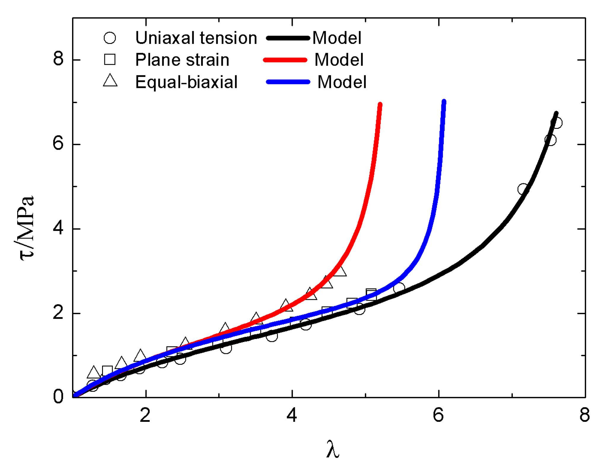
• A robust model should not only simulate one kind of experiment, for instance, uniaxial tension, but also others.
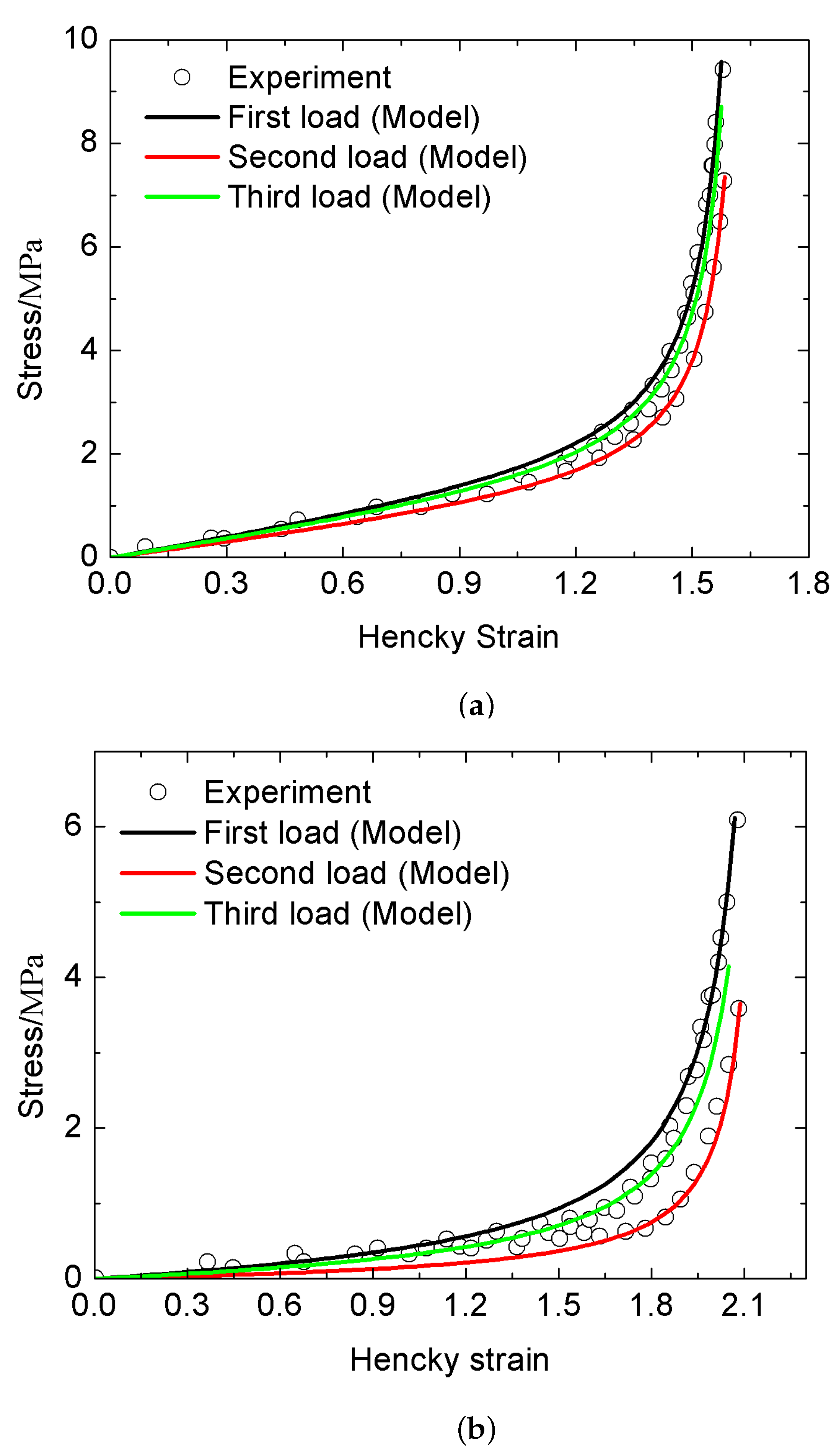
• A unified form should be given out to exactly match the test data under first loading, second loading, and third loading after thermal annealing.

The purpose of this article is to establish a compressible multi-axial potential with thermodynamic consistency to model the three benchmark tests of uniaxial tension/compression, equal-biaxial tension/compression, and plane strain tension/compression in the processes of first loading, second loading, and third loading after thermal annealing. A departure from the previous studies in [25,26], Wang et al. [27], Yuan et al. [28], and Xiao et al. [29] is that two new parameters are introduced into the new model: one parameter characterizing energy dissipation to account for stress softening in the second loading, and another one called weight factor that represents the percentage of recovery of the Mullins effect.

The paper is arranged as follows: First, a compressible multi-axial strain energy function is established using three specific invariants based on the stress–strain curves in the three benchmark tests. Second, it is demonstrated that the new model satisfies thermodynamic laws by giving out the explicit formulations of the Helmholtz free energy and the entropy. Third, a unified shape function with energy dissipation and weight factor is proposed to capture the properties of stress softening and thermal recovery of the Mullins effect. Finally, numerical results are obtained to compare with the test data. Finally, concluding remarks are given out.

2. New Potential

The definitions of the symbols used in this article are shown in

Table 1. Definitions for symbols.

Symbol	Definition	Symbol	Definition
$\mathit{F}$	Deformation gradient	$\mathit{B}$	Left Cauchy–Green tension
$\mathbf{\tau }$	Kirchhoff Stress	$\mathbf{\sigma }$	Cauchy–Green tension
J	Volumetirc ratio	$\nu$	Poisson ratio
W	Potential	$\mathit{h}$	Hencky strain
$\tilde{\mathbf{h}}$	Deriatoric Hencky strain	$\mathit{I}$	Second-order identity tensor
T	Temperature	$\mathit{D}$	Stretching
$\phi$	Internal energy per unit	$\mathit{q}$	Heat flowing
r	Heat supply	$\eta$	Specific entropy
$\psi$	Helmholtz free energy	℘	Internal dissipation

.

It is widely accepted that the strain with Hencky type is more direct for deducing the Kirchhoff stress than any other types, as shown in Fitzjerald [30], Xiao [31], and Hill [32]. Kirchhoff stress can be derived from an elastic potential in terms of the Hencky strain $\mathit{h}$ in a broad sense to consider the temperature as follows:

$$\dot{\mathbf{\tau }}=\frac{\partial {\mathit{W}}^{\mathit{2}}}{\partial {\mathit{h}}^2}:\dot{\mathit{h}}+\frac{\partial {\mathit{W}}^{\mathit{2}}}{\partial \mathit{h}\partial T}\dot{T}.$$

(1)

When the temperature is constant, we have

$$\mathbf{\tau }=\frac{\partial \mathit{W}}{\partial \mathit{h}}.$$

(2)

Here, the Hencky strain $\mathit{h}$ is expressed by

$$\mathit{h}=\sum _{r=1}^3(\ln {\lambda }_r){\mathit{n}}_r\otimes {\mathit{n}}_r,$$

(3)

${\lambda }_1,{\lambda }_2,{\lambda }_3$ are the three principal stretches and ${\mathit{n}}_1,{\mathit{n}}_2,{\mathit{n}}_3$ are the three corresponding orthonormal principal axis vectors (Eulerian triad); W is the compressible multi-axial strain energy potential, which depends on the Hencky strain $\mathit{h}$ and the dissipation energy $\kappa$,

$$W=W(\mathit{h},\kappa ).$$

(4)

It is assumed that the variants $\mathbf{\tau }$ and $\kappa$ are independent. The relationship between the Cauchy stress $\mathbf{\sigma }$ and Kirthhoff stress $\mathbf{\tau }$ is

$$\mathbf{\tau }=\mathit{J}\mathbf{\sigma }.$$

(5)

Towards the goal of establishing compressible multi-axial potential, three steps need to be completed:

• One-dimensional potentials in three benchmark tests need to be derived from the their corresponding stress–strain relationships.
• Three specific invariants need to be introduced to capture the compressible condition, and to expand the one-dimensional potentials into a unified, multi-axial potential.
• It needs to be proven that the new potential can automatically reduce to the one-dimensional case.

2.1. One-Dimensional Potentials

Let the one-dimensional stress–strain relationships in uniaxial, and equal-biaxial be separately given by:

$${\tau }_u=f_u(h,\kappa ).$$

(6)

$${\tau }_e=f_e(h,\kappa ).$$

(7)

In the case of plane strain, the stress–strain relationship in the loaded direction is given by:

$${\tau }_p=g(h,\kappa ),$$

(8)

and in the fixed direction, we have:

$${\overline{\tau }}_p=\widehat{g}(h,\kappa ),$$

(9)

The explicit formulations of Equations (6), (8) and (9) may be determined by the test data by means of rational interpolation, which will be explained in the following context. Additionally, Equation (7) can be deduced from Equation (6), as shown in Xiao et al. [29].

Three one-dimensional potentials may be separately derived from Equations (6)–(8), and we obtain

$$w_u(h,\kappa )={\int }_0^h(f_u(h,\kappa ))dh,$$

(10)

$$w_e(h,\kappa )={\int }_0^h(f_e(h,\kappa ))dh,$$

(11)

$$w_p(h,\kappa )={\int }_0^h(g(h,\kappa ))dh.$$

(12)

2.2. Specific Invariants

In order to account for the compressible condition and expand one-dimensional potentials into a unified multi-axial potential, three specific invariants based on the Hencky stress are introduced by

$${\gamma }_1=i_1=ln(J),$$

(13)

$${\gamma }_2=\sqrt{\frac{2}{3}{j}_2},$$

(14)

$${\gamma }_3=\sqrt{6}\frac{j_3}{j_2^{1.5}},$$

(15)

where,

$$i_s=tr({\mathit{h}}^s),$$

(16)

$$j_s=tr({\tilde{\mathit{h}}}^s),$$

(17)

$s=1,2,3$. $j_s$ can be derived from $i_s$ as follows:

$$j_2=i_2-\frac{1}{3}{i}_1^2,$$

(18)

and

$$j_3=i_3-i_1{i}_2+\frac{2}{9}{i}_1^3.$$

(19)

We briefly describe the three invariants as follows:

• ${\gamma }_1$ is introduced to account for how the volume changes. If the rubber-like material is incompressible, we have ${\gamma }_1=0$.
• ${\gamma }_2$ is introduced to bridge the one-dimensional case and the multi-axial case. ${\gamma }_2$ becomes the Hencky strain h at the one-dimensional case.
• ${\gamma }_3$ is introduced to combine the one-dimension potentials into a unified multi-axial potential. We separately have ${\gamma }_3=-1$, 0, and 1 in the case of uniaxial compression, plane strain, and uniaxial tension.

By using the three specific invariants ${\gamma }_1,{\gamma }_2,$, and ${\gamma }_3,$ instead of the Hencky stress $\mathit{h}$, Equation (2) may be expressed as

$$\mathbf{\tau }=\frac{\partial \mathit{W}}{\partial {\gamma }_1}\mathit{I}+\frac{2}{3}\frac{\partial \mathit{W}}{\partial {\gamma }_2}{\gamma }_2^{-1}\tilde{\mathit{h}}+\frac{\partial \mathit{W}}{\partial {\gamma }_3}\check{\mathit{h}},$$

(20)

where,

$$\check{\mathit{h}}=4{\gamma }_2^{-3}\tilde{\mathit{h}}-2{\gamma }_2^{-2}\tilde{\mathit{h}}-2{\gamma }_2^{-1}\mathit{I}.$$

(21)

The three tensors $\mathit{I},\tilde{\mathit{h}},\check{\mathit{h}}$ are mutually orthogonal in the sense of:

$$\left\{\begin{array}{c}\mathit{I}:\tilde{\mathit{h}}=\mathbf{0},\hfill \\ \mathit{I}:\check{\mathit{h}}=\mathbf{0},\hfill \\ \check{\mathit{h}}:\tilde{\mathit{h}}=\mathbf{0}.\hfill \end{array}\right.$$

(22)

Therefore, the three tensors $\mathit{I},\tilde{\mathit{h}},\check{\mathit{h}}$ form an orthogonal basis for the isotropic tensor function of the Hencky strain $\mathit{h}$.

2.3. Compressible Multi-Axial Potential

A compressible multi-axial potential may be derived from the one-dimensional potentials and the specific invariants by using a generalized procedure of Hermite interpolation, as shown in Yuan et al. [28] and Xiao et al. [29], which accounts for the energy dissipation. The new unified potential is expressed as follows:

$$W=\frac{1-2\nu }{3}{w}_u(\frac{{\gamma }_1}{1-2\nu },\kappa )+\frac{1+\nu }{6}[Z_{+}{(1+{\gamma }_3)}^2+Z_{-}{(1-{\gamma }_3)}^2],$$

(23)

with $Z_{+}$ and $Z_{-}$ taking the forms of:

$$Z_{+}=(2-{\gamma }_3)w_u(\frac{3/2{\gamma }_2}{1+\nu },\kappa )+({\gamma }_3-1)Y_{+},$$

(24)

$$Z_{-}=(2+{\gamma }_3)w_u(\frac{-3/2{\gamma }_2}{1+\nu },\kappa )+({\gamma }_3+1)Y_{-},$$

(25)

and $Y_{+}$ and $Y_{-}$ taking the forms of:

$$\left\{\begin{array}{c}{Y}_{+}=\frac{5}{2}{w}_u(\frac{3/2{\gamma }_2}{1+\nu },\kappa )-\frac{1}{2}{w}_u(-\frac{3/2{\gamma }_2}{1+\nu },\kappa )-2w_p(\frac{3\sqrt{3}{\gamma }_2}{4(1+\nu )},\kappa )-G,\hfill \end{array}\right.$$

(26)

$$\left\{\begin{array}{c}{Y}_{-}=\frac{1}{2}{w}_u(\frac{3/2{\gamma }_2}{1+\nu },\kappa )-\frac{5}{2}{w}_u(-\frac{3/2{\gamma }_2}{1+\nu },\kappa )+2w_p(\frac{3\sqrt{3}{\gamma }_2}{4(1+\nu )},\kappa )-G,\hfill \end{array}\right.$$

(27)

with

$$G=\frac{\sqrt{3}{\gamma }_2}{4(1+\nu )}(g(\frac{3\sqrt{3}{\gamma }_2}{4(1+\nu )},\kappa )-2\widehat{g}(\frac{3\sqrt{3}{\gamma }_2}{4(1+\nu )},\kappa )).$$

(28)

$\nu$ is the Poisson ratio, which can be expressed by

$$\nu =-\frac{\overline{h}}{h}$$

(29)

where $\overline{h}$ is the lateral Hencky strain. Equations (23)–(28) form the compressible multi-axial potential in the sense of capturing the property of strain softening and thermal recovery of the Mullins effect.

2.4. Predictions for One-Dimensional Cases

Predictions for the three benchmark tests should be given to ensure the effectiveness of the new potential. Three specific invariants, ${\gamma }_1,{\gamma }_2$, and ${\gamma }_3$ in the one-dimensional case are presented in

Table 2. Prediction for the benchmark tests (“t/c” means “tension/compression”).

Quantity	Uniaxial t/c	Biaxial t/c	Plane Strain
${\gamma }_1$	$(1-2\nu )h$	$(2-1/\nu )h$	$\frac{1-2\nu }{1-\nu }h$
${\gamma }_2$	$\frac{2}{3}(1+\nu )h$	$\frac{2}{3}(1+1/\nu )h$	$\frac{2}{\sqrt{3}}h$
${\gamma }_3$	1/−1	−1/1	0

.

Substituting the values ${\gamma }_1,{\gamma }_2$, and ${\gamma }_3$ into Equations (23)–(28), we obtain the one-dimensional potential, volume ratio, and stress–strain relationship in each benchmark test, as shown in

Table 3. Prediction for the benchmark tests (“t/c” means “tension/compression”).

Quantity	Uniaxial t/c	Biaxial t/c	Plane Strain
W	$w_u(h,\kappa )$	$w_e(h,\kappa )$	$w_p(h,\kappa )$
J	${\lambda }^{1-2\nu }$	${\lambda }^{\frac{2\nu -1}{\nu }}$	${\lambda }^{\frac{1-2\nu }{1-\nu }}$
$\tau$	$f_u(h,\kappa )$	$f_e(h,\kappa )$	$g(h,\kappa )$ and $\widehat{g}(h,\kappa )$

.

The stress–stain relationship in the equal-axial case can be determined from Equation (6); as shown in Xiao et al. [29], we obtain the stress in the loaded direction of the equal-axial case as follows:

$$\tau =f_e(h,\kappa )=-\frac{{\nu }^{-1}}{2}{f}_u(-{\nu }^{-1}h,\kappa )$$

(30)

We may conclude from Table 3 that the new potential can automatically reduce to Equation (6) in the uniaxial case, Equation (7) in the equal-axial case, and Equations (8) and (9) in the plane strain case. All the stress–strain relationships in the three benchmark tests may be determined by Equations (6), (8) and (9), whose explicit formulations will be given according to the test data in the following sections.

3. Thermodynamic Consistency

Explicit formulations for the Helmholtz free energy and the entropy are given to ensure that the new model satisfies thermodynamic conditions. We follow the steps in Xiao et al. [33]. Substituting

$$\dot{\mathit{h}}=\mathit{D}$$

(31)

into the thermodynamic laws, we have

$$\dot{\phi }=\mathbf{\tau }:\dot{\mathit{h}}-J▽·\mathit{q}+r$$

(32)

and

$$\dot{\eta }\ge -J▽\frac{\mathit{q}}{T}+\frac{r}{T}$$

(33)

where, $\mathit{D}$ is the stretching, defined by

$$\mathit{D}=\frac{1}{2}(\dot{\mathit{F}}·{\mathit{F}}^{-1}+{(\dot{\mathit{F}}·{\mathit{F}}^{-1})}^T)$$

(34)

Moreover, ▽ is used to designate the formal differentiation vector with respect to the current position vector x, namely,

$$▽=\frac{\partial }{\partial x}$$

(35)

$\phi$ represents the internal energy per unit, $\mathit{q}$ is the heat flow, r is the heat supply, and $\eta$ is the specific entropy. The internal dissipation ℘ is defined by

$$\wp =T\dot{\eta }-(r-J▽·\mathit{q}).$$

(36)

The Helmholtz free energy $\psi$ is given by

$$\psi =\phi -T\eta .$$

(37)

According to Equations (32)–(35), we have

$$\wp =\mathbf{\tau }:\dot{\mathit{h}}-(\dot{\psi }+\eta \dot{T}).$$

(38)

The thermodynamic laws require that

$$\wp \ge 0.$$

(39)

Towards this goal, the explicit formulations for the Helmholtz free energy and the entropy are given as follows

$$\psi ={\psi }_0+\frac{\partial W}{\partial \mathit{h}}:\mathit{h}-W+\kappa +{\int }_0^{\kappa }(-\frac{{\partial }^{2}W}{\partial \mathit{h}\partial \kappa }:\mathit{h}+\frac{\partial W}{\partial \kappa })d\kappa$$

(40)

$$\eta =-{\psi }_0^{\prime }+\frac{\partial W}{\partial T}$$

(41)

where the term ${\psi }_0={\psi }_0(T)$ characterizes the specific heat capacity of the material. The demonstration for Equations (40) and (41) fulfil the thermodynamic laws, shown as follows: Taking the derivative of $\psi$ with respect to time, we obtain

$$\dot{\psi }=\frac{\partial \psi }{\partial \mathit{h}}:\dot{\mathit{h}}+\frac{\partial \psi }{\partial T}\dot{T}+\frac{\partial \psi }{\partial \kappa }\dot{\kappa }$$

(42)

The formulations of $\frac{\partial \psi }{\partial \mathit{h}}$, $\frac{\partial \psi }{\partial T}$, and $\frac{\partial \psi }{\partial \kappa }$ can be determined from Equation (40),

$$\frac{\partial \psi }{\partial \mathit{h}}=\frac{{\partial }^{2}W}{\partial {\mathit{h}}^2}:\mathit{h}$$

(43)

$$\frac{\partial \psi }{\partial T}={\psi }_0^{\prime }+\frac{{\partial }^{2}W}{\partial \mathit{h}\partial T}:\mathit{h}-\frac{\partial W}{\partial T}$$

(44)

and

$$\frac{\partial \psi }{\partial \kappa }=1$$

(45)

Substituting Equations (43)–(45) into Equation (42), we have

$$\dot{\psi }=\frac{{\partial }^{2}W}{\partial {\mathit{h}}^2}:\mathit{h}:\dot{\mathit{h}}+({\psi }_0^{\prime }+\frac{{\partial }^{2}W}{\partial \mathit{h}\partial T}:\mathit{h}-\frac{\partial W}{\partial T})\dot{T}+\dot{\kappa }$$

(46)

Substituting Equations (46) and (41) into Equation (38), and combing Equation (1), we have

$$\wp =\dot{\kappa }$$

(47)

This is because $\dot{\kappa }$ is always greater than or equal to 0, we obtain $\wp \ge 0$. The proof is completed.

4. Shape Functions with Stress Softening and Thermal Recovery

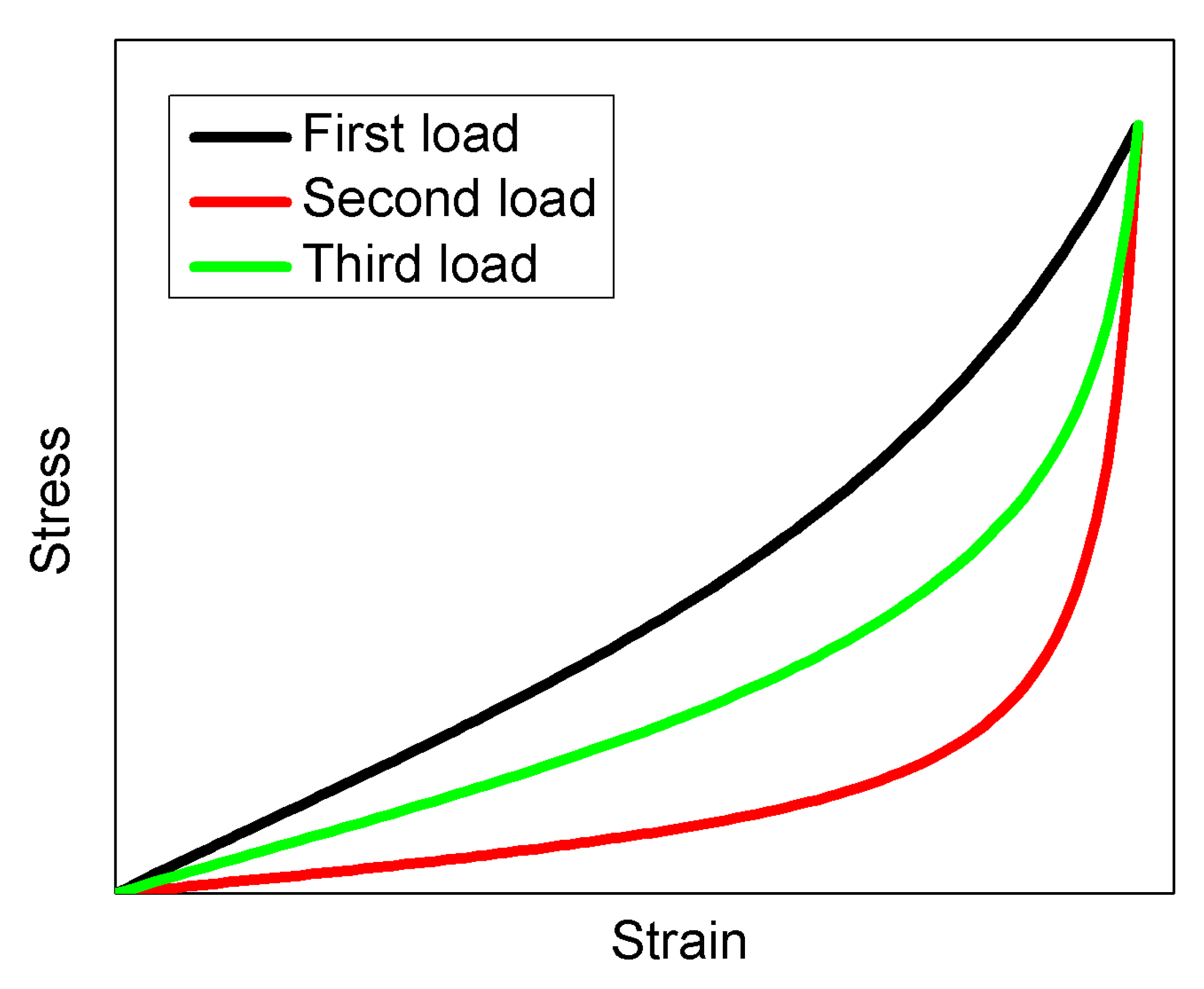
Towards our goal, the one-dimensional shape functions $\tau =f_u(h,\kappa )$, $\tau =g(h,\kappa )$, and $\tau =\widehat{g}(h,\kappa )$ need to be given based on the test data. Additionally, the dissipation energy $\kappa$ is introduced to account for stress softening, and the weight factors ${\beta }_i$, $i=1,2,3$, are introduced to explain the thermal recovery of the Mullins effect. The shape functions are given by

$$f_u(h,\kappa )={\beta }_1{f}_1(h)+(1-{\beta }_1)f_2(h,\kappa ),$$

(48)

$$g(h,\kappa )={\beta }_2{g}_1(h)+(1-{\beta }_2)g_2(h,\kappa ),$$

(49)

and

$$\widehat{g}(h,\kappa )={\beta }_3{\widehat{g}}_1(h)+(1-{\beta }_3){\widehat{g}}_2(h,\kappa ).$$

(50)

According to Equations (27) and (48), we have

$$f_e(h,\kappa )=-\frac{{\nu }^{-1}}{2}[{\beta }_1{f}_1(-{\nu }^{-1}h)+(1-{\beta }_1)f_2(-{\nu }^{-1}h,\kappa )].$$

(51)

As shown in Figure 1, when a rubber bar first loads, the stress–strain curve moves along the black line, which is denoted by $f_1(h)$ in the uniaxial case, $g_1(h)$ in the loaded direction in the plane strain case, or ${\widehat{g}}_1(h)$ in the fixed direction in the plane strain case. When the stress reaches a certain value, the unloading process begins until the stress reaches zero. After that, the bar reloads and the stress–strain curve moves along the red line, which is denoted by $f_2(h,\kappa )$ in the uniaxial case, $g_2(h,\kappa )$ in the loaded direction in the plane strain case, or ${\widehat{g}}_2(h,\kappa )$ in the fixed direction in the plane strain case. When the bar reloads again after the thermal recovery of the Mullins effect, the stress–strain curve moves along the green line, which lies between the black line and the red line.

The meanings of the weight factors ${\beta }_i$, $i=1,2,3$ are as follows:

• When ${\beta }_i=1$, $i=1,2,3$, the shape functions become $f_u(h,\kappa )=f_1(h)$, $g(h,\kappa )=g_1(h)$, $\widehat{g}(h,\kappa )={\widehat{g}}_1(h)$, and $f_e(h,\kappa )=-\frac{{\nu }^{-1}}{2}{f}_1(-{\nu }^{-1}h)$, which means that the stress–strain curve moves along the black line on the virgin specimen.
• When ${\beta }_i=0$, $i=1,2,3$, the shape functions become $f_u(h,\kappa )=f_2(h,\kappa )$, $g(h,\kappa )=g_2(h,\kappa )$, $\widehat{g}(h,\kappa )={\widehat{g}}_2(h,\kappa )$, and $f_e(h,\kappa )=-\frac{{\nu }^{-1}}{2}{f}_2(-{\nu }^{-1}h,\kappa )$, which means the stress–strain curve moves along the red line for the specimen with stress softening.
• When $0<{\beta }_i<1$, $i=1,2,3$, and the shape functions are represented by (36)–(39), and they move along the green line for the specimen after the treatment of thermal recovery.
• The weight factors ${\beta }_i=1$, $i=1,2,3$ in the range from 0 to 1 represent the percentage of recovery, which means the larger the weight factor, the higher the percentage of recovery of the Mullins effect.

The expression of $\kappa$ can be provided by analyzing the experimental results of the Mullins effect in Mullins [3], Diani et al. [34], and Dorfmann and Ogden [12]. The following observation results are obtained from the Mullins effect. First, the stress–strain curve is lower than the primary loading path during the process of unloading, i.e., strain softening. This phenomenon becomes more obvious in the case of a large unloading stress. Second, we pay direct attention to one cycle; the area of the hysteresis loop only represents the energy dissipation, and it will accumulate during the process of the loading–unloading cycles. Third, the permanent set may be ignored for some specific rubber samples.

Based on the above analysis, the explicit formulation for $\kappa$ may be given by

$$\kappa =\frac{{\kappa }_m}{2}[\tan \mathrm{h}(m({\tau }_m-{\tau }_r))+1].$$

(52)

Here,

$${\kappa }_m={\int }_0^{{\overline{f}}^{-1}({\tau }_m)}\overline{f}(h)dh,$$

(53)

is the work performed by the primary path flow (virgin stress–strain curve). m and ${\tau }_r$ are parameters whose values can be determined from test data. ${\tau }_m$ is the unloading stress. If ${\tau }_m={\tau }_c$, we have $\kappa =\frac{1}{2}{\kappa }_m$. $h={\overline{f}}^{-1}(\tau )$ is the inverse function of $\tau =\overline{f}(h)$. With $\tau ={\tau }_m$, we obtain the value of ${\overline{f}}^{-1}({\tau }_m)$. $\overline{f}(h)$ becomes $f_1(h)$ in the case of uniaxial, and $g_1(h)$ in the case of plane strain.

According to Equation (52), when the unloading stress is small enough, for example, ${\tau }_m\approx 0$, we obtain $\kappa \approx 0$, and the subsequent path and the primary path almost coincide. When the unloading stress is large enough, for example, ${\tau }_m>>{\tau }_r$, we obtain $\kappa \approx {\kappa }_m$, and the materials are extremely softened.

5. Numerical Results

According to the symmetry property of the test data, the explicit formulations for the shape functions of Equations (48)–(50) may be given by using the method of rational interpolation. Two kinds of experiments are chosen for model validation, which are three benchmark tests for one rubber-like sample, as shown in Treloar [35], Jones and Treloar [36], and Yohsuke et al. [37], and experiments with stress softening and thermal recovery, as shown in Harwood and Payne [21].

5.1. Explicit Shape Functions via Rational Interpolation

Based on the method of rational interpolation, the explicit formulations of $f_1(h)$, $f_2(h,\kappa )$, $g_1(h)$, $g_2(h,\kappa )$, ${\widehat{g}}_1(h)$, and ${\widehat{g}}_2(h,\kappa )$ in Equations (48)–(50) may be given by:

$$f_1(h)=E_{0}h(\frac{{\alpha }_{u0}}{(1-\frac{h}{h_{e0}})(1+\frac{h}{h_{c0}})}+1-{\alpha }_{u0}),$$

(54)

$$f_2(h,\kappa )=E(\kappa )h[\frac{{\alpha }_u(\kappa )}{(1-\frac{h}{h_e(\kappa )})(1+\frac{h}{h_c(\kappa )})}+1-{\alpha }_u(\kappa )],$$

(55)

$$g_1(h)=\frac{2}{3}{E}_{0}h(\frac{{\alpha }_{p0}}{1-\frac{h^2}{h_{p0}^2}}+1-{\alpha }_{p0}),$$

(56)

$$g_2(h,\kappa )=\frac{2}{3}E(\kappa )h[\frac{{\alpha }_p(\kappa )}{1-\frac{h^2}{{(h_p(\kappa ))}^2}}+1-{\alpha }_p(\kappa )],$$

(57)

$${\widehat{g}}_1(h)=\frac{1}{3}{E}_{0}h(\frac{{\widehat{\alpha }}_{p0}}{1-\frac{h^2}{h_{p0}^2}}+1-{\widehat{\alpha }}_{p0}),$$

(58)

and

$${\widehat{g}}_2(h,\kappa )=\frac{1}{3}E(\kappa )h[\frac{{\widehat{\alpha }}_p(\kappa )}{1-\frac{h^2}{{(h_p(\kappa ))}^2}}+1-{\widehat{\alpha }}_p(\kappa )].$$

(59)

When the material first loads, ${\beta }_i=1$, $i=1,2,3$, and the shape functions of Equations (49)–(52) may separately reduce to $f_1(h)$, $g_1(h)$, ${\widehat{g}}_1(h)$, and $-\frac{{\nu }^{-1}}{2}{f}_1(-{\nu }^{-1}h)$, which can be determined from Equations (54), (56) and (58). Therefore, the parameters of $E_0$, ${\alpha }_{u0}$, $\nu ,h_{e0}$, $h_{c0}$, ${\alpha }_{p0}$, $h_{p0}$, and ${\widehat{\alpha }}_{p0}$ in these equations need to be determined. When the second material loads after stress softening, ${\beta }_i=0$, $i=1,2,3$, the shape functions of Equations (49)–(52) may separately reduce to $f_2(h,\kappa )$, $g_2(h,\kappa )$, ${\widehat{g}}_2(h,\kappa )$, and $-\frac{{\nu }^{-1}}{2}{f}_2(-{\nu }^{-1}h,\kappa )$, which can be determined from Equations (55), (57) and (59). Therefore, the parameter functions $E(\kappa )$, ${\alpha }_u(\kappa )$, $h_e(\kappa )$, $h_c(\kappa )$, ${\alpha }_p(\kappa )$, $h_p(\kappa )$, ${\widehat{\alpha }}_p(\kappa )$ in these equations need to be provided according to the value of $\kappa$, which can be determined from Equation (52) by choosing the appropriate values of m and ${\tau }_c$. When the third material loads after the thermal recovery, $0<{\beta }_i<1$, $i=1,2,3$, the shape functions in Equations (48)–(52) need to be determined by choosing the appropriate values of $E_0$, ${\alpha }_{u0}$, $\nu ,h_{e0}$, $h_{c0}$, ${\alpha }_{p0}$, $h_{p0}$, and ${\widehat{\alpha }}_{p0}$ in Equations (54), (56) and (58), suitable formulations of $E(\kappa )$, ${\alpha }_u(\kappa )$, $h_e(\kappa )$, $h_c(\kappa )$, ${\alpha }_p(\kappa )$, $h_p(\kappa )$, ${\widehat{\alpha }}_p(\kappa )$ in Equations (55), (57) and (59) according to the value of $\kappa$, which can be deduced from Equation (49) using the appropriate parameters of m and ${\tau }_c$. Furthermore, an appropriate value of ${\beta }_i$, $i=1,2,3$ in the range from 0 to 1 is necessary.

5.2. Results for the Benchmark Tests

The values of the parameters $E_0$, ${\alpha }_{u0}$, $h_{e0}$, $h_{c0}$, ${\alpha }_{p0}$, $h_{p0}$, ${\widehat{\alpha }}_{p0}$ are given in

Table 4. Parameter value for matching benchmark tests.

Experiment	${\mathit{E}}_0/$MPa	$\mathit{\nu }$	${\mathit{h}}_{\mathit{e}0}$	${\mathit{h}}_{\mathit{c}0}$	${\mathit{\alpha }}_{\mathit{u}0}$	${\mathit{\alpha }}_{\mathit{p}0}$	${\widehat{\mathit{\alpha }}}_{\mathit{p}0}$	${\mathit{h}}_{\mathit{p}0}$
Treloar [35]	1	$0.499$	$2.14$	$3.66$	2	$1.5$	/	$1.95$
Jones and Treloar [36]	$1.3$	$0.499$	$2.4$	$3.74$	3	13	$-10$	$4.7$
Yohsuke et al. [37]	$2.3\times {10}^{-3}$	$0.499$	$1.92$	$3.22$	2	5	$8.5$	$2.71$

to fit the three benchmark test data of Treloar (1975), Jones and Treloar (1975), and Yohsuke et al. (2011).

Putting $h=ln(\lambda )$ into the specific functions, the comparisons between the model and the test data are shown in Figure 2, Figure 3 and Figure 4.

Here, ${\tau }_p$ and ${\overline{\tau }}_p$ are separately the stress in the loading direction and fixed direction in the case of plane strain.

5.3. Results for Tests with Stress Softening and Thermal Recovery

In what follows, the experiment of Harwood and Payne [21] with stress softening and thermal recovery of the Mullins effect is chosen for model validation. The samples include three type A vulcanizates (polysulfide crosslinks with 4.17% sulfur, 2.5% sulfur, and 1.25% sulfur), three type B vulcanizates (monosulfide crosslinks with 0.6% sulfur, 0.4% sulfur, and 0.2% sulfur), and two type C vulcanizates (carbon–carbon crosslinks with 3.5% dicumyl peroxide and 0.5% dicumyl peroxide). The following steps are adopted for each sample:

• The parameters $E_0$, ${\alpha }_{u0}$, $h_{e0}$, and $h_{c0}$, are determined by the first load curve.
• The appropriate parameters of m, and ${\tau }_c$ in Equation (49) are given to determined the value of $\kappa$ using the unloading stress in the test.
• The values for the parameter functions of $E(\kappa )$, ${\alpha }_u(\kappa )$, $h_e(\kappa )$, and $h_c(\kappa )$ are determined by the second load curve. Conversely, formulations of these parameter functions can be deduced by the method of interpolation with the initial values of $E_0$, ${\alpha }_{u0}$, $h_{e0}$, and $h_{c0}$, respectively.
• The weight factors ${\beta }_i$, $i=1,2,3$ in each sample can be determined by the third load curve.

The parameters $E_0$, ${\alpha }_{u0}$, $h_{e0}$, and $h_{c0}$ are shown in

Table 5. Parameter values for a matching test of type A vulcanizates in Harwood and Payne [21] in virgin load.

Vulcanizates	${\mathit{E}}_0/$MPa	${\mathit{h}}_{\mathit{e}0}$	${\mathit{h}}_{\mathit{c}0}$	${\mathit{\alpha }}_{\mathit{u}0}$
$4.17\%$ sulfur	$1.83$	$1.59$	10	$0.28$
$2.5\%$ sulfur	$1.02$	$1.75$	10	$0.45$
$1.25\%$ sulfur	$0.7$	$1.9$	10	$0.3$

,

Table 6. Parameter values for matching test of type B vulcanizates in Harwood and Payne [21] in virgin load.

Vulcanizates	${\mathit{E}}_0/$MPa	${\mathit{h}}_{\mathit{e}0}$	${\mathit{h}}_{\mathit{c}0}$	${\mathit{\alpha }}_{\mathit{u}0}$
$0.6\%$ sulfur	$1.77$	$1.6$	10	$0.13$
$0.4\%$ sulfur	$0.92$	$1.74$	10	$0.38$
$0.2\%$ sulfur	$0.66$	$1.9$	10	$0.3$

and

Table 7. Parameter values for matching test of type C vulcanizates in Harwood and Payne [21] in virgin load.

Vulcanizates	${\mathit{E}}_0/$MPa	${\mathit{h}}_{\mathit{e}0}$	${\mathit{h}}_{\mathit{c}0}$	${\mathit{\alpha }}_{\mathit{u}0}$
$3.5\%$ dicup	$1.3$	$1.64$	10	$0.18$
$0.5\%$ dicup	$0.28$	$2.194$	10	$0.7$

for vulcanizates of types A, B, and C in Harwood and Payne [21].

${\tau }_m$ is the unloading stress and needs to be determined from the experimental data. Appropriate values of m and ${\tau }_c$ are chosen to determine the ${\kappa }_1$ after stress softening. The values of the shape functions $E({\kappa }_1)$, ${\alpha }_u({\kappa }_1)$, $h_e({\kappa }_1)$, and $h_c({\kappa }_1)$ can be determined from the test data. Then, the explicit formulations of these functions need to be determined by using the method of interpolation with the initial values given in Table 5, Table 6 and Table 7. Finally, ${\beta }_1$ can be determined from the test data after thermal recovery. The values of ${\tau }_m$, m, ${\tau }_c$, ${\kappa }_1$, $E({\kappa }_1)$, ${\alpha }_u({\kappa }_1)$, $h_e({\kappa }_1)$, $h_c({\kappa }_1)$, and ${\beta }_1$ are given in

Table 8. Parameter values for matching test of type A vulcanizates in Harwood and Payne [21] with stress softening and thermal recovery.

Vulcanizates	${\mathit{\tau }}_{\mathit{m}}$	m	${\mathit{\tau }}_{\mathit{c}}$	${\mathit{\kappa }}_1$	$\mathit{E}({\mathit{\kappa }}_1)$	${\mathit{h}}_{\mathit{e}}({\mathit{\kappa }}_1)$	${\mathit{h}}_{\mathit{c}}({\mathit{\kappa }}_1)$	${\mathit{\alpha }}_{\mathit{u}}({\mathit{\kappa }}_1)$	${\mathit{\beta }}_1$
$4.17\%$ sulfur	$10.26$	$0.2$	$11.72$	$1.188$	$1.30$	$1.58$	10	$0.20$	$0.25$
$2.5\%$ sulfur	$10.26$	$0.2$	$10.53$	$1.481$	$0.88$	$1.75$	10	$0.18$	$0.34$
$1.25\%$ sulfur	$10.26$	$0.2$	$9.98$	$1.280$	$0.20$	$1.98$	10	$1.00$	$0.40$

,

Table 9. Parameter values for matching test of type B vulcanizates in Harwood and Payne [21] with stress softening and thermal recovery.

Vulcanizates	${\mathit{\tau }}_{\mathit{m}}$	m	${\mathit{\tau }}_{\mathit{c}}$	${\mathit{\kappa }}_1$	$\mathit{E}({\mathit{\kappa }}_1)$	${\mathit{h}}_{\mathit{e}}({\mathit{\kappa }}_1)$	${\mathit{h}}_{\mathit{c}}({\mathit{\kappa }}_1)$	${\mathit{\alpha }}_{\mathit{u}}({\mathit{\kappa }}_1)$	${\mathit{\beta }}_1$
$0.6\%$ sulfur	$9.78$	$0.2$	$11.68$	$0.950$	$1.20$	$1.65$	10	$0.17$	$0.75$
$0.4\%$ sulfur	$9.78$	$0.2$	$11.63$	$0.835$	$0.88$	$1.72$	10	$0.15$	$0.55$
$0.2\%$ sulfur	$9.78$	$0.2$	$9.85$	$1.150$	$0.30$	$1.93$	10	$0.50$	$0.60$

and

Table 10. Parameter values for matching test of type C vulcanizates in Harwood and Payne [21] with stress softening and thermal recovery.

Vulcanizates	${\mathit{\tau }}_{\mathit{m}}$	m	${\mathit{\tau }}_{\mathit{c}}$	${\mathit{\kappa }}_1$	$\mathit{E}({\mathit{\kappa }}_1)$	${\mathit{h}}_{\mathit{e}}({\mathit{\kappa }}_1)$	${\mathit{h}}_{\mathit{c}}({\mathit{\kappa }}_1)$	${\mathit{\alpha }}_{\mathit{u}}({\mathit{\kappa }}_1)$	${\mathit{\beta }}_1$
$0.35\%$ dicup	$9.84$	$0.2$	$12.59$	$0.66$	$1.0$	$1.65$	10	$0.18$	$0.67$
$0.50\%$ dicup	$6.12$	$0.2$	$5.69$	$0.96$	$0.1$	$2.17$	10	$0.8$	$0.60$

separately for the vulcanizates of types A, B, and C.

Comparison between experimental data and model result are shown in Figure 5, Figure 6 and Figure 7.

6. Concluding Remarks

A compressible, multi-axial potential is proposed to exactly match the three benchmark tests for rubber-like materials, considering the stress softening and thermal recovery of the Mullins effect. We conclude the article as follows:

(1)

The specific invariant ${\gamma }_1$ is introduced to account for the general compressible deformation mode. Actually, the compressible condition can not be ignored under some deformation modes, such as the hydrostatic pressure. Additionally, the constraint of incompressibility may also give rise to convergence problems in finite element code, as shown in Biscoff et al. [38]. Therefore, it is necessary to establish a new model considering compressible deformation.

(2)

The new model is multi-axial and can fit all of the three benchmark tests, i.e., uniaxial, equal-biaxial, and plane strain, by introducing another two invariants of ${\gamma }_2$ and ${\gamma }_3$.

(3)

The thermodynamic laws are fulfilled by explicitly providing the appropriate formulations of the Helmholtz free energy in Equation (40) and the specific entropy in Equation (41).

(4)

All of the parameters in the new model are explicitly decided, instead of being implicitly provided via complex iterative calculation.

(5)

Both stress softening and thermal recovery can be accounted for in the new model by the dissipation energy $\kappa$ and the weight factors ${\beta }_i$, $i=1,2,3$.

References

1. Mullins, L. Effect of stretching on the properties of rubber. J. Rubber. Res. 1948, 21, 281–300. [Google Scholar] [CrossRef]
2. Mullins, L. Softening of rubber by deformation. Rubber Chem. Technol. 1969, 42, 339–362. [Google Scholar] [CrossRef]
3. Mullins, L.; Tobin, N.R. Theoretical model for the elastic behaviour of filler-reinforced vulcanized rubbers. Rubber Chem. Technol. 1957, 30, 551–571. [Google Scholar] [CrossRef]
4. Qi, H.J.; Boyce, M.C. Constitutive model for stretch-induced softening of the stress-stretch behavior of elastomeric. J. Mech. Phys. Solids 2004, 52, 2187–2205. [Google Scholar] [CrossRef]
5. Arruda, E.M.; Boyce, M.C. A three-dimensional constitutive model for the large stretch behavior of elastomers. J. Mech. Phys. Solids 1993, 41, 389–412. [Google Scholar] [CrossRef] [Green Version]
6. Miehe, C.; Keck, J. Superimposed fnite elastic-viscoelastic-plastoelastic response with damage in filled rubbery polymers. Experiments, modeling and algorithmic implementation. J. Mech. Phys. Solids 2000, 48, 323–365. [Google Scholar] [CrossRef]
7. Simo, J.C. On a fully three-dimensional finite-strain viscoelastic damage model: Formulation and computational aspects. Comput. Methods Appl. Mech. Engrg. 1987, 60, 153–173. [Google Scholar] [CrossRef]
8. Kachanov, L.M. Time of the rupture process under creep conditions, Izy Akad. Nauk. Ssr Otd Tekh Nauk. 1958, 58, 26–31. [Google Scholar]
9. Li, J.; Mayau, D.; Lagarrigue, V. A constitutive model dealing with damage due to cavity growth and the Mullins effect in rubber-like materials under triaxial loading. J. Mech. Phys. Solids 2008, 56, 953–973. [Google Scholar] [CrossRef]
10. Beatty, M.F.; Krishnaswamy, S. A theory of stress-softening in incompressible isotropic materials. J. Mech. Phys. Solids 2000, 48, 1931–1965. [Google Scholar] [CrossRef]
11. Laiarinandrasana, L.; Piques, R.; Robisson, A. Visco-hyperelastic model with internal state variable coupled with discontinuous damage concept under total Lagrangian formulation. Int. J. Plast. 2003, 19, 977–1000. [Google Scholar] [CrossRef]
12. Dorfmann, A.; Ogden, R.W. A constitutive model for the Mullins effect with permanent set in particle-reinforced rubber. Int. J. Solids Struct. 2004, 41, 1855–1878. [Google Scholar] [CrossRef]
13. Ogden, R.W.; Roxburgh, D.G. A pseudo-elastic model for the Mullins effect in filled rubber. Proc. R Soc. Lond A 1999, 455, 2861–2877. [Google Scholar] [CrossRef]
14. Horgan, C.O.; Ogden, R.W.; Saccomandi, G. A theory of stress softening of elastomers based on finite chain extensibility. Proc. R Soc. Lond A 2004, 460, 1737–1754. [Google Scholar] [CrossRef]
15. Sreejith, P.; Kannan, K.; Rajagopal, K.R. A thermodynamic framework for additive manufacturing, using amorphous polymers, capable of predicting residual stress, warpage and shrinkage. Int. J. Eng. Sci. 2021, 159, 103412. [Google Scholar] [CrossRef]
16. Trentadue, F.; De Tommasi, D.; Puglisi, G. A predictive micromechanically-based model for damage and permanent deformations in copolymer sutures. J. Mech. Behav. Biomed. Mater. 2021, 115, 104277. [Google Scholar] [CrossRef]
17. Fazekas, B.; Goda, T.J. Constitutive modelling of rubbers: Mullins effect, residual strain, time-temperature dependence. Int. J. Mech. Sci. 2021, 210, 106735. [Google Scholar] [CrossRef]
18. Rigbi, Z. Reinforcement of rubber by carbon black. Prop. Polym. 1980, 55, 21–68. [Google Scholar]
19. Laraba-Abbes, F.; Ienny, P.; Piques, R. A new ’tailor-made’ methodology for the mechanical behaviour analysis of rubber-like materials: II. application to the hyperelastic behaviour characterization of a carbon-black filled natural rubber vulcanizate. Polymer 2003, 44, 821–840. [Google Scholar] [CrossRef]
20. Yan, L.; Dillard, D.A.; West, R.L.; Lower, L.D.; Gordon, G.V. Mullins effect recovery of a nanoparticle-filled polymer. J. Polym. Sci. Part Polym. Physics 2010, 48, 2208–2214. [Google Scholar] [CrossRef]
21. Harwood, J.; Payne, A. Stress softening in natural rubber vulcanizates. iv. unfilled vulcanizates. Rubber Chem. Technol. 1967, 40, 840–848. [Google Scholar] [CrossRef]
22. Hanson, D.E.; Hawley, M.; Houlton, R.; Chitanvis, K.; Rae, P.; Orler, E.B.; Wrobleski, D.A. Stress softening experiments in silica-filled polydimethylsiloxane provide insight into a mechanism for the Mullins effect. Polymer 2005, 46, 10989–10995. [Google Scholar] [CrossRef]
23. Drozdov, A.D.; Dorfmann, A. Stress-softening and recovery of elastomers. arXiv 2001, arXiv:0102052. [Google Scholar]
24. Wang, S.L.; Chester, S.A. Modeling thermal recovery of the Mullins effect. Mech. Mater. 2018, 126, 88–98. [Google Scholar] [CrossRef]
25. Xiao, H. An explicit, direct approach to obtaining multi-axial elastic potentials that exactly match data of four benchmark tests for rubberlike materials-part 1: Incompressible deformations. Acta Mech. 2012, 223, 2039–2063. [Google Scholar] [CrossRef]
26. Xiao, H. An explicit, direct approach to obtain multi-axial elastic potentials which accurately match data of four benchmark tests for rubbery materials part 2: General deformations. Acta Mech. 2013, 224, 479–498. [Google Scholar] [CrossRef]
27. Wang, X.M.; Li, H.; Yin, Z.N.; Xiao, H. Multiaxial strain energy functions of rubberlike materials: An explicit approach based on polynomial interpolation. Rubber Chem. Technol. 2014, 87, 168–183. [Google Scholar] [CrossRef]
28. Yuan, L.; Gu, Z.X.; Yin, Z.N.; Xiao, H. New compressible hyperelastic models for rubberlike matereials. Acta Mech. 2015, 226, 4059–4072. [Google Scholar] [CrossRef]
29. Xiao, H.; Ding, X.F.; Cao, J.; Yin, Z.N. New multi-axial constitutive models for large elastic deformation behaviors of soft solids up to breaking. Int. J. Solids Struct. 2017, 109, 123–130. [Google Scholar] [CrossRef]
30. Fitzjerald, S. A tensorial Hencky measure of strain and strain rate for finite deformation. J. Appl. Phys. 1980, 51, 5111–5115. [Google Scholar] [CrossRef]
31. Xiao, H. Hencky strain and Hencky model: Extending history and ongoing tradition. Multidiscip. Model. Mater. Struct. 2005, 1, 1–52. [Google Scholar] [CrossRef]
32. Hill, R. Constitutive inequalities for isotropic elastic solids under finite strain. Proc. R. Soc. Lond. A 1970, 326, 131–147. [Google Scholar]
33. Xiao, H.; Bruhns, O.T.; Meyers, A. Thermodynamic laws and consistent Eulerian formulation of finite elastoplasticity with thermal effects. J. Mech. Phys. Solids 2007, 55, 338–365. [Google Scholar] [CrossRef]
34. Diani, J.; Brieu, M.; Vacherand, J.M. A damage directional constitutive model for Mullins effect with permanent set and induced anisotropy. Eur. J. Mech. A/Solids 2006, 25, 483–496. [Google Scholar] [CrossRef]
35. Treloar, L.R.G. The Physics of Rubber Elasticity; Oxford University Press: Oxford, UK, 1975. [Google Scholar]
36. Jones, D.F.; Treloar, L.R.G. The properties of rubber in pure homogeneous strain. J. Phys. D 1975, 8, 1285–1304. [Google Scholar] [CrossRef]
37. Yohsuke, B.; Urayama, K.; Takigawa, T.; Ito, K. Biaxial strain testing of extremely soft polymer gels. Soft Matter 2011, 7, 2632–2638. [Google Scholar] [CrossRef]
38. Biscoff, J.E.; Arrude, E.M.; Grosh, K.A. A new constitutive model for the compressibility of elastomers at finite deformation. Rubber Chem. Technol. 2001, 74, 541–559. [Google Scholar] [CrossRef]
Figure 1. Schematic description for tress softening and thermal recovery.
Symmetry 14 02663 g001
Figure 2. Comparison between model result and the experimental data in Treloar [35], x axis represents the stretch ratio λ , and y axis represents the Kirchhoff stress τ .
Symmetry 14 02663 g002
Figure 3. Comparison between model result and the experimental data in Jones and Treloar [36], x axis represents the stretch ratio λ , and y axis represents the Kirchhoff stress τ .
Symmetry 14 02663 g003
Figure 4. Comparison between model result and experimental data in Yohsuke et al. [37], x axis represents the stretch ratio λ , and y axis represents the Kirchhoff stress τ .
Symmetry 14 02663 g004
Figure 5. Model calibration of Type A vulcanizate with different amounts of crosslinker in Harwood and Payne [21]. (a) Vulcanizate with 4.17% sulfur; (b) Vulcanizate with 2.5% sulfur; (c) Vulcanizate with 1.25% sulfur.
Symmetry 14 02663 g005
Figure 6. Model calibration of Type B vulcanizate with different amounts of crosslinker in Harwood and Payne [21]. (a) Vulcanizate with 0.6% sulfur; (b) Vulcanizate with 0.4% sulfur; (c) Vulcanizate with 0.2% sulfur.
Symmetry 14 02663 g006
Figure 7. Model calibration of Type C vulcanizate with different amounts of crosslinker in Harwood and Payne [21]. (a) Vulcanizate with 3.5% dicumyl peroxide; (b) Vulcanizate with 0.5% dicumyl peroxide.
Symmetry 14 02663 g007