A Domain-Adversarial Multi-Graph Convolutional Network for Unsupervised Domain Adaptation Rolling Bearing Fault Diagnosis

Abstract

The transfer learning method, based on unsupervised domain adaptation (UDA), has been broadly utilized in research on fault diagnosis under variable working conditions with certain results. However, traditional UDA methods pay more attention to extracting information for the class labels and domain labels of data, ignoring the influence of data structure information on the extracted features. Therefore, we propose a domain-adversarial multi-graph convolutional network (DAMGCN) for UDA. A multi-graph convolutional network (MGCN), integrating three graph convolutional layers (multi-receptive field graph convolutional (MRFConv) layer, local extreme value convolutional (LEConv) layer, and graph attention convolutional (GATConv) layer) was used to mine data structure information. The domain discriminators and classifiers were utilized to model domain labels and class labels, respectively, and align the data structure differences through the correlation alignment (CORAL) index. The classification and feature extraction ability of the DAMGCN was significantly enhanced compared with other UDA algorithms by two example validation results, which can effectively achieve rolling bearing cross-domain fault diagnosis.

1. Introduction

With the booming machine manufacturing industry, rotating machinery has been extensively used in various industries. As an indispensable, core component of rotating machinery, the run status of the rolling bearing has considerable influence on the safety of rotating machinery [1]. In order to avoid major disasters, safety incidents, and economic losses that may result from the failure of rotating machinery, the timely diagnosis of failing technology is of particular relevance, and we should pay close attention to the running conditions of rotating machinery [2,3].

There are usually two types of bearing fault diagnosis models: the model-driven diagnosis method and the data-driven diagnosis method. The model-driven method needs to establish an accurate diagnosis model based on acquired prior knowledge for fault diagnosis and identification. For relatively small datasets, traditional model-driven diagnosis technology can achieve good results. Lee et al. [4] proposed an asymmetric intradomain alignment (AIIDA) fault diagnosis method under different domain displacement conditions and verified the effectiveness and superiority of the proposed model through various scenarios in three bearing datasets. Qiu et al. [5] proposed a weak feature detection method based on wavelet filtering for rolling bearing fault prediction, which has a good prediction effect on bearing defect signals and smooth signals. Yuan et al. [6] proposed a semi-supervised multi-graph joint embedding (SMGJE) model to better characterize the structural relationship of data in high-dimensional spaces and successfully applied it to the field of rotor fault diagnosis.

Conventional fault diagnosis methods based on machine learning (ML) perform well in processing small datasets but perform poorly when dealing with large batches of data [7,8,9]. Moreover, traditional methods rely heavily on feature engineering background knowledge and expert experience, and they extract features mainly via manual operations, which makes them very limited when dealing with relatively large datasets. The deep learning (DL) method has gradually turned into one of the most prevalent fault diagnosis technologies at present [10,11]. In contrast, the deep learning method has the capability of learning deeper feature representations from large-scale data and can effectively mine the complex mapping relationship between features and data, thus heightening the performance of fault diagnosis methods [12]. For instance, many methods, such as convolutional neural networks (CNN) [13], deep belief networks (DBN) [14], recurrent neural networks (RNN) [15], and long short-term memory networks (LSTM) [16] can achieve excellent diagnosis results for the different fault types of rolling bearings.

Although the study of fault diagnosis models based on DL is in full swing, the fact that these methods still have some defects cannot be ignored. There are, mainly, two aspects: (1) Most DL-based methods default to the probability distribution of the data in the source and target domain being identical. However, in the real industrial environment, the machine-running conditions change in real-time on account of factors such as equipment health and the inevitable presence of external interference [17]. This may lead to some distribution differences among the obtained data, so the above assumption does not hold. (2) The DL model often relies on a great deal of labeled data in order to perform training. However, in various industrial applications, the proportion of labeled samples in large-scale data is quite small, and it is nearly impossible to label all data due to cost and expertise constraints. If abundant labeled data are not provided for training, these methods are undoubtedly useless, which largely restricts the application of DL-based intelligent fault diagnosis methods in related industries [18].

To overcome these shortcomings, unsupervised domain adaptation (UDA) [19] techniques have been proposed as a solution, which can adjust data distribution through acquired domain-invariant features and shared discriminative features and transfer the data mapping relationship derived from the source domain labeled data to the unlabeled target domain, so as to use the source domain’s operating conditions to assist in diagnosing the unknown types of faults in the target domain operating conditions. UDA technologies have been widely used in recent years, and they can be roughly divided into the following four categories: network-based methods, mapping-based methods, instance-based methods, and adversarial-based methods [20]. For example, Deng et al. [21] proposed the relative maximum mean difference (RMMD) distance criterion to align source and target domain data more precisely to construct an unsupervised fault diagnosis model. Wang et al. [22] designed a deep domain-adversarial network integrating Wasserstein distance to achieve fault diagnosis under changing operational conditions. Che et al. [23] developed a novel domain-adaptive DBN framework with an improved maximum mean difference (MMD) in order to achieve domain adaptation alignment.

Understanding the structural information in data contributes to reducing data distribution discrepancies and keeping data attributes in the original space for the better construction of migration relationships between source and target domains [24]. Many current UDA methods only take into account the influence of class labels and domain labels but ignore the fact that data structure is also a crucial class of information, so it is also necessary to integrate the data structure information model into UDA-based fault diagnosis methods. Traditional deep neural networks (DNN) have difficulty modeling data structure information, so graph convolutional networks (GCN) are introduced to map data geometric structure information relationships and implement model construction [25,26]. Li et al. [27] proposed the multi-receptive field graph convolutional network (MRF-GCN) for fault classification, which achieved information aggregation for different sensory fields. Yang et al. [28] designed a feature extraction method called Super Graph and successfully applied it to fault diagnosis.

For the sake of improving the mining of deep structure information in data, we have designed a multi-graph convolutional network (MGCN) that integrates three graph convolutional layers: a multi-receptive field graph convolutional (MRFConv) layer [27], a local extreme value convolutional (LEConv) layer [29], and a graph attention convolutional (GATConv) layer [30]. This effectively allows us to extract information from different numbers of nodes and their local extremum information, where the introduction of GATConv can ascertain the importance of different neighbor nodes in order to avoid losing important information during the above convolution. Based on the above work, a domain-adversarial multi-graph convolutional network (DAMGCN) for UDA is developed to construct a rolling bearing variable condition fault diagnosis model. Firstly, the fault features are extracted from the original input signal by using ResNet-18. Second, the graph model is formed by excavating the relationship between the sample structural features. Finally, MGCN is utilized to further acquire the structural feature of the sample data to model the instance graph. Structural alignment loss based on the correlation alignment (CORAL) [31] metric is introduced to determine the structural differences between the two domains. Integrating data structure modeling information into UDA techniques not only allows us to extract domain-invariant and shared discriminative features but also enables high-performance cross-domain fault diagnosis.

The main contributions of this paper are summarized as follows.

(1)

We propose a novel multi-graph convolution network architecture that integrates three different graph convolution layers (an MRFConv layer, LEConv layer, and GATConv layer) to extract the deep effective structural features of bearing data.

(2)

On the basis of MGCN, we have constructed a graph transfer learning framework for variable condition fault diagnosis, which defines the sample classification loss, domain alignment loss, and structure alignment loss to achieve high-precision variable condition fault type identification.

(3)

Two examples are given to illustrate the effectiveness and superiority of the proposed model in the context of fault diagnosis under variable working conditions.

The rest of this paper is structured as follows. Section 2 briefly introduces the basic principles of UDA and graph convolutional networks (GCNs). In Section 3, the proposed cross-domain fault diagnosis model of DAMGCN is described. In Section 4, sufficient cross-domain diagnosis examples and process analyses are presented to test and verify the performance of the DAMGCN in cross-domain fault diagnosis. Finally, a comprehensive summary of the full paper is made in Section 5.

2. Theoretical Background

2.1. Unsupervised Domain Adaptation

In recent years, more and more UDA models have been proposed, among which, mapping- and confrontation-based methods are the most widely used. For example, a series of methods, including MMD [32], multi-core MMD [33], and CORAL [31], belong to mapping-based methods. Among the confrontation-based methods, methods such as number domain confrontation neural network (DANN) [34] and condition domain-adversarial network (CDAN) [35] are commonly used. The CORAL method is a very simple and clear UDA method. It uses the idea of linear transformation to align the second-order statistics distributed in the source domain and the target domain and minimizes the covariance difference in cross-domain learning features; it effectively solves the UDA scenario problem in the target domain without marked data. In classification problems, traditional DANN may not be able to effectively align the complex multimodal distribution structure, while CDAN can build an adversarial adaptation model based on the shared discriminative information, and the key part of the model lies in the conditional domain discriminator, based on the cross-entropy of the domain feature representation and the classifier prediction result. Thus, the complex multi-modal structure can be better identified, the characteristics of the two domains can be accurately distinguished, and the cross-domain fault identification problem can be realized.

2.2. Graph Convolutional Network

Define a basic graph, $G=\left(V,\epsilon ,A\right)$, arbitrarily, where $V=\left\{V_1,V_2,\dots ,V_N\right\}$ refers to a finite set of $N$ nodes in the graph, $G$; $\epsilon$ refers to a finite set of $N$ edges of the graph $G$; and $A\in R^{N\times N}$ refers to the adjacency matrix between the vertices of the graph. If any two nodes $\langle v_i,v_j\rangle$ in the graph, $G$, are connected, then we have $A_{ij}=1$; otherwise, $A_{ij}=0$. The Laplacian matrix, $L$, is described as follows:

$$L=D-A$$

(1)

where $D_{ii}={\displaystyle {\sum }_j{A}_{ij}}$ is the diagonal matrix of the graph.

Further, the symmetric normalization operation of the $L$ is defined as

$$L=D^{-1/2}L{D}^{-1/2}=I_N-D^{-1/2}A{D}^{-1/2}=U\mathsf{\Lambda }{U}^{-1}$$

(2)

where $I_N$ denotes the unit matrix; $\mathsf{\Lambda }=diag\left(\left[{\lambda }_1,{\lambda }_2,\dots ,{\lambda }_N\right]\right)$ denotes the diagonal matrix composed of the eigenvalues, ${\lambda }_i$, of $L$; and $U=\left(u_1,u_2,\dots ,u_N\right)$ denotes the orthogonal matrix composed of the eigenvectors, $u_i$, of $L$.

Therefore, the spectral convolution between the node and the feature, $x$, is shown below:

$$g={\left(x{*}_{G}f\right)}_{\theta }=U\left(U^{T}x{U}^{T}f\right)=U{f}_{\theta }{U}^{T}x$$

(3)

where $f$ denotes the eigenfunction of the diagonal matrix $\mathsf{\Lambda }$, $\theta$ denotes the learnable parameter, ${*}_G$ denotes the graph convolution operator, and $f_{\theta }=U^{T}f$ denotes the graph convolution filter.

According to reference [36], to deal with the problem wherein computing the features of $L$ is very expensive and time-consuming, Hammond et al. proposed that the graph convolution operation can be well approximated to the $k\mathrm{th}$ order via a truncated expansion of Chebyshev polynomials, as follows:

$$f_{{\theta }^{\prime }}={\displaystyle \sum _{k=0}^{K-1}{\theta }_k{\mathsf{\Lambda }}^k=}{\displaystyle \sum _{k=0}^{K-1}{\theta }^{\prime }{}_k}{C}_k\left(\tilde{\mathsf{\Lambda }}\right)$$

(4)

where $\tilde{\mathsf{\Lambda }}=\frac{2\mathsf{\Lambda }}{{\lambda }_{\max }}-I_N$ denotes the diagonal matrix of rescaled eigenvalues, ${\lambda }_{\max }$ means the maximum eigenvalue of $L$, $K$ is the maximum order of the Chebyshev polynomial, and ${\theta }_k^{\prime }\in R^K$ is now transformed into a vector of Chebyshev coefficients. The filter is approximated by the Chebyshev polynomial $C_k\left(x\right)=2x{C}_{k-1}\left(x\right)-C_{k-2}\left(x\right),C_0\left(x\right)=1\mathrm{and}{C}_1\left(x\right)=0$, and further, Equation (3) can be derived as

$$g={\displaystyle \sum _k^{K-1}{\theta }_k^{\prime }}{C}_k\left(\tilde{L}\right)x$$

(5)

where $\tilde{L}=\frac{2L}{{\lambda }_{\max }}-I_N$ denotes the rescaled graph’s Laplacian matrix. The ReLU activation function is usually introduced to perform the nonlinear activation of the graph convolution results:

$$z=\mathrm{ReLU}\left({\displaystyle \sum _k^{K-1}{\theta }_k^{\prime }}{C}_k\left(\tilde{L}\right)x\right)$$

(6)

In turn, graph node classification can be achieved using the softmax function.

$$Z=\mathrm{softmax}\left(g\left(\mathrm{ReLU}\left(g\left(X,A\right)\right),A\right)\right)$$

(7)

where $X=\left\{x_1,x_2,\dots x_N\right\}$ denotes the node feature, and $Z$ denotes the output graph convolution signal matrix. The simple three-layer GCN model is defined in Figure 1.

3. DAMGCN Cross-Domain Fault Diagnosis Model

3.1. MGCN

From the above, it can be seen that the graph filter in GCN can be approximated by $K$-order Chebyshev polynomials, so the graph’s Laplacian matrix is also $K$-localized; namely, GCN is the $K$-order receptive field. $K$ is generally taken as one in traditional graph convolutional (GConv) layers, which means that it extracts data features from the nodes themselves and cannot learn multi-domain information that better characterizes the graph data, and the GConv layers focus on all nodes in the whole perceptual field range, leading them to neglect the importance of local node information. Therefore, in order to acquire information from multiple receptive fields and focus on the impact of local nodes on the whole graph model, a hybrid graph convolutional network integrating three convolutional layers (an MRFConv layer, LEConv layer, and GATConv layer) is designed in this paper, as shown in Figure 2. Further, the introduction of the GATConv layer to MGCN can ascertain the weight of different neighboring nodes and discriminate the importance of different neighboring nodes. Moreover, traditional GCNs generally use the ReLU activation function, but considering that ReLU can easily make the backpropagation gradient zero when the feature value is less than zero, the LeakyReLU activation function is used in MGCN to circumvent this defect.

The MRFConv layer is designed to address the problem wherein the traditional GConv layer can only aggregate the node information from a fixed neighborhood and cannot take into account all the nodes in the whole graph, and it includes a few parallel GConv layers with different receptive field sizes, which can effectively extract the information from neighboring nodes in different receptive fields and greatly enhance the output feature representation capability. Therefore, the node feature matrix, $X$, of the graph, $G$, for MRFConv operation with a maximum-range perceptual field of three is defined as follows:

$$\begin{array}{ll}{H}_1& =\left[{\displaystyle \sum _{k_1=0}^{K_1-1}{\theta }_{k_1}^{\prime }{C}_{k_1}\left(\tilde{L}\right)}X,{\displaystyle \sum _{k_2=0}^{K_2-1}{\theta }_{k_2}^{\prime }{C}_{k_2}\left(\tilde{L}\right)}X,{\displaystyle \sum _{k_3=0}^{K_3-1}{\theta }_{k_3}^{\prime }{C}_{k_3}\left(\tilde{L}\right)}X\right]\\ & =\left[\stackrel{K_1-1}{A}X{W}_1,\stackrel{K_2-1}{A}X{W}_2,\stackrel{K_3-1}{A}X{W}_3\right]\end{array}$$

(8)

where $[·]$ represents the concatenation operator; ${\theta }_{k_1}^{\prime },{\theta }_{k_2}^{\prime },{\theta }_{k_3}^{\prime }$ denote the weight parameters of the three GConv layers with the sensory field size of $K_1,K_2,K_3$, respectively; $W_1,W_2,W_3$ are the corresponding weight parameter matrix; and $H_1$ represents the features aggregated by MRFConv layers.

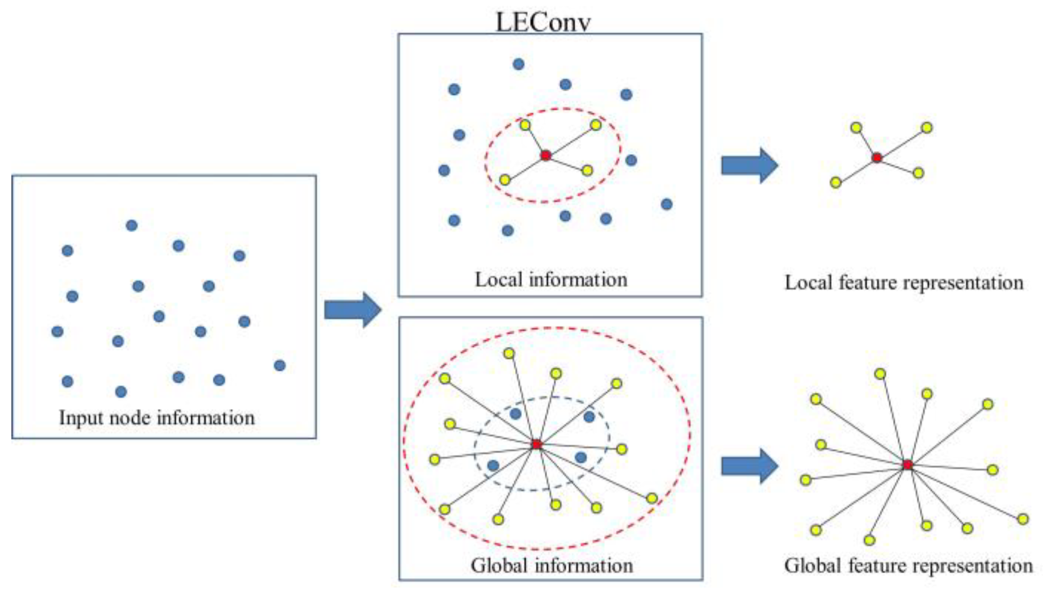
The node features after convolution aggregation by the MRFConv layer already contain rich information. However, the MRFConv layer only focuses the target on different sizes of the receptive field and does not take into account the local node information within the same receptive field, which will lead to the insufficient mining of local node information by the convolutional operation and then affect the local information representation capability of the convolutional output features. The LEConv layer can comprehensively consider the global and local importance between the node itself and its neighbors. By performing clustering operations, it can mine and process the global and local information of feature nodes and avoid an adverse impact on model performance caused by the loss of local information. The convolution operation of LEConv is shown in Figure 3. It performs the LEConv operation on the original input node information and can perform convolution clustering on the local information and the global information of the node and effectively extract local and global feature representations from the node. Therefore, the LEConv layer is used to perform local clustering operations on all the possibilities of the three different receptive field ranges in MRFConv to extract local node extreme value feature information. The specific operations of LEConv are defined as follows:

$$H_2=\left(x_i{W}_1+{\displaystyle \sum _{j\in N\left(i\right)}{A}_{i,j}\left(x_i{W}_2-x_j{W}_3\right)}\right)$$

(9)

where $x_i,x_j$ refers to the two adjacent node features, $A_{i,j}$ refers to the adjacency matrix elements between nodes $i$ and $j$, $N$ indicates the number of nodes, and $H_2$ denotes the local extreme value features extracted by the LEConv layer.

Moreover, it is worth noting that both the MRFConv layer and LEConv layer have difficulty allocating different learning weights to different neighbor nodes, and all neighbor nodes are treated equally. However, in the actual scenario, different neighbor nodes may play different roles on the core node, so they cannot be simply generalized. To better handle this problem, the GATConv layer is introduced to achieve the adaptive matching of weights to different neighbor nodes and then obtain their respective importance relative to the core nodes to prevent the loss of important information caused by ignoring the differences in node weights during the convolution process. The GATConv operation is shown below:

$$\begin{array}{l}{H}_3={\displaystyle \sum _{j\in N\left(i\right)}{\alpha }_{i,j}W{x}_j}\\ {\alpha }_{i,j}={\mathrm{softmax}}_i\left(e_{ij}\right)\\ e_{ij}=\mathrm{LeakyReLU}\left({\overrightarrow{a}}^T\left[W{x}_i|W{x}_j\right]\right)\end{array}$$

(10)

where $\overrightarrow{a}\in R^{N\times N}$ indicates single-layer feedforward neural network, and $W$ is the importance of the weight matrix between different neighbor nodes learned by GATConv.

In summary, the overall graph convolution operation in MGCN can be defined as

$$H=\left[H_1,H_2,H_3\right]$$

(11)

where $[·]$ stands for the concatenation operator.

3.2. DAMGCN

This subsection investigates the application of the MGCN in UDA fault diagnosis proposed above, which aims to mine the domain-invariant and shared discriminant feature representations from the source domain, rich in fault feature information, and then apply it to the transfer fault diagnosis task of unlabeled target domains. Let the source domain space be defined as $Q_s={\left\{\left(x_i^s,y_i^s\right)\right\}}_{i=1}^{n_s}$, where $x_i^s$ and $y_i^s$ are the source domain data and their corresponding category labels, respectively, and $n_s$ denotes the amount of source domain labeled data. Correspondingly, let the space of the target domain be defined as $Q_t={\left\{\left(x_i^t\right)\right\}}_{i=1}^{n_t}$, where $x_i^t$ denotes the target domain unlabeled data feature, and $n_t$ denotes the amount of target domain unlabeled data. Define $x_i^s\in X_s,x_i^t\in X_t$ as the sample space of the source and target domain and $y_i^s\in Y_s,Y_t$ as the label space of the source and target domain. Generally, in UDA, the label space of two domains is considered to show no difference ($Y_s=Y_t$), and the sample spaces are related but different from each other ($X_s\ne X_t$). The objective of our research is to construct the proposed MGCN as a DAMGCN in the context of UDA with the following mapping relation, $f_{DAMGCN}:X_t\to Y_t$, to predict the labels of the unlabeled samples of the target domain based on the labeled information of the source domain and to achieve cross-domain fault diagnosis in UDA.

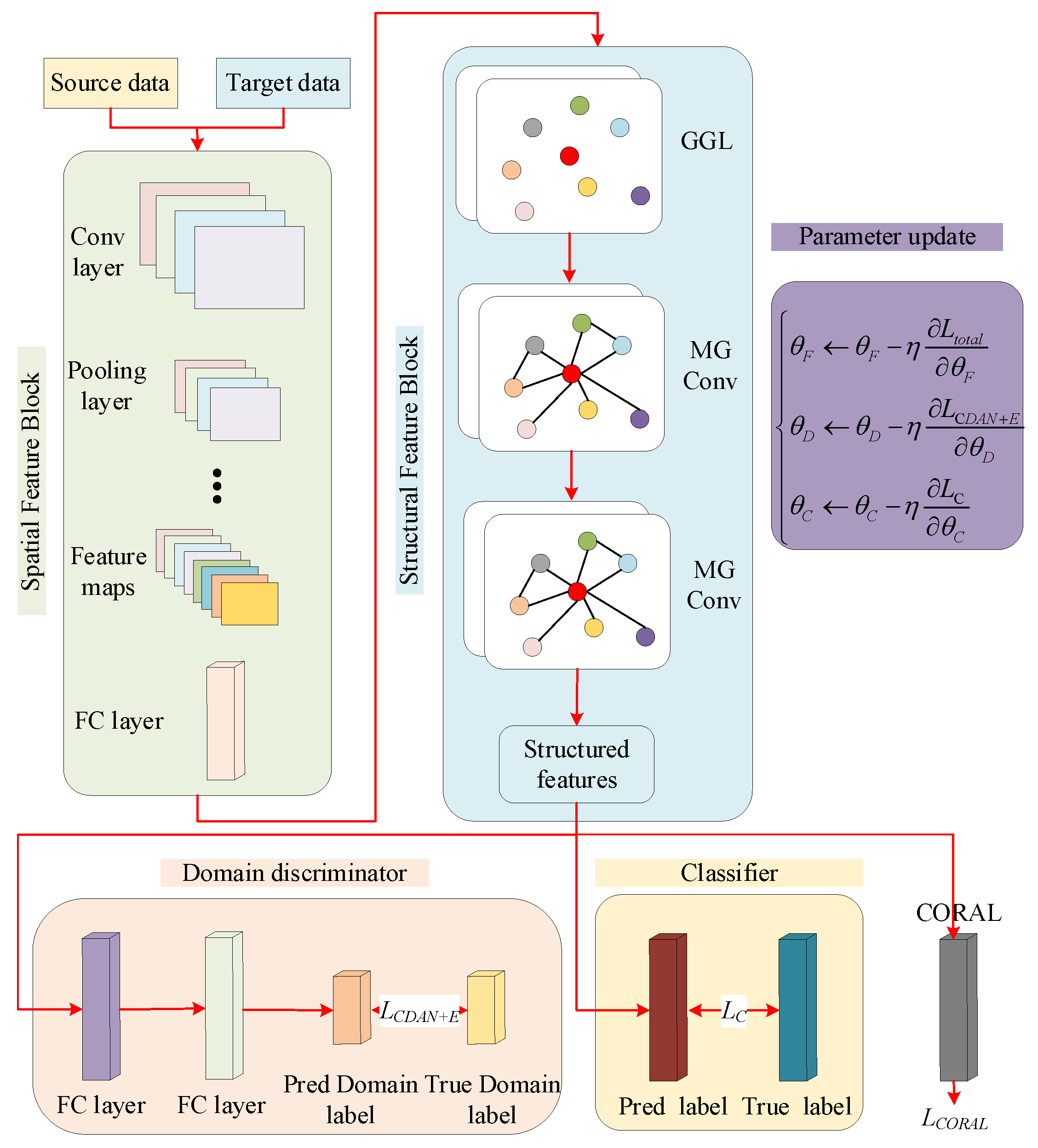
DAMGCN is a new network architecture based on ResNet-18 and MGCN. The architecture diagram of the developed DAMGCN for a rolling bearing fault diagnosis network under changing working conditions is given in Figure 4. The network consists of four main parts: the ResNet-18 spatial feature extractor, the MGCN structural feature extractor, the domain discriminator, and the classifier. First, the original data are input into the ResNet-18 for training to obtain the spatial features of the data, where a feature vector is regarded as a node and the specific values of the feature vectors are regarded as node features. The extracted nodes and node features are then automatically generated using a graph generation layer (GGL) [24] to provide suitable input graph data for the MGCN. Afterward, the graphs obtained via GGL are input into the MGCN for enhanced structure information extraction to extract node features containing rich data structural information. Finally, the data structural node features extracted from the MGCN are input into the domain discriminator for domain-adversarial training to minimize the differences in data structure distribution so that the classifier can classify different fault types more accurately. The GGL provides MGCN with two important components of the graph: the adjacency matrix, $A$, and the node feature matrix, $X$. The $X$ can be extracted from the original input data by ResNet-18, and the $A$ is calculated by the GGL. The $X$ operation rules are defined as follows:

$$X=\mathrm{ResNet}18\left(X_{input}\right)$$

(12)

where $X_{input}$ represents the original input data matrix.

After extracting a small batch of node feature matrixes from the original input matrix via ResNet-18, the extracted feature matrix is input into the GGL for graph construction. The specific construction process is as follows.

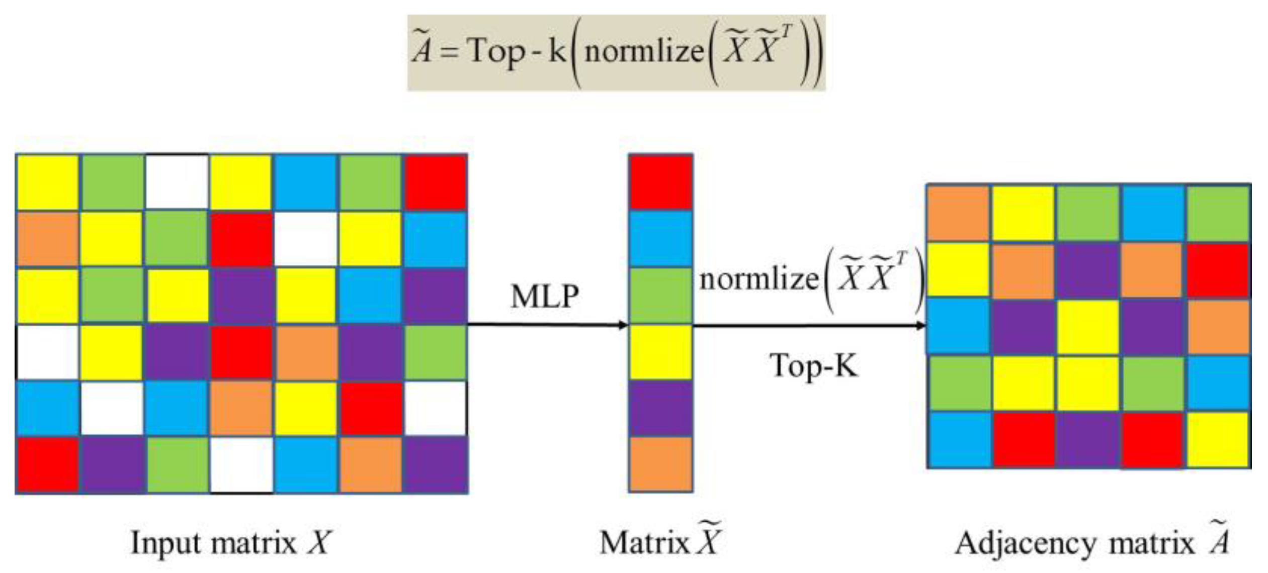
Firstly, the extracted node feature matrix, $X$, is fed into the MLP neural network, and the processed node feature matrix, $\tilde{X}$, can be obtained with the MLP. Secondly, the adjacency matrix, $A$, can be obtained via the matrix multiplication of $\tilde{X}$ and $\tilde{X}$ transposition and normalization. Thus, the adjacency matrix, $A$, is calculated as follows:

$$\{\begin{array}{l}\tilde{X}=\mathrm{MLP}\left(X\right)\\ A=\mathrm{normlize}\left(\tilde{X}{\tilde{X}}^T\right)\end{array}$$

(13)

where $\tilde{X}$ refers to the MLP-transformed node feature matrix, and $\mathrm{normlize}(·)$ refers to the normalization function.

Finally, considering that the original input data are too large, the adjacency matrix will be too complicated, which may affect the computational speed and cost. Therefore, the Top-k mechanism is introduced to sparse the adjacency matrix by selecting the Top-k nearest neighbors of each node.

$$\tilde{A}=Top-k\left(A\right)$$

(14)

where $\tilde{A}$ denotes the final sparse adjacency matrix obtained, and then, in the next step, a graph convolution operation is performed on the graph consisting of $\tilde{A}$ and $\tilde{X}$. Similar to the pooling operation of CNN, in the graph structure, the Top-k function extracts the index of the first $k$ maximum values of matrix $A$ in the row direction; it can achieve the purpose of sparsing the graph structure by filtering out useful nodes, where the $k\mathrm{th}$ element represents the total number of nodes in the first $k-1\mathrm{th}$ subgraphs. Therefore, in Equation (14), the original adjacency matrix, $A$, can be TOP-k processed, and its useful elements can be retained to obtain a sparse adjacency matrix, where we define $k$ as the length of the first dimension of the adjacency matrix. The adjacency matrix and node feature matrix needed to construct a graph dataset are obtained using the GGL method, and then, the required MGCN graph structure can be obtained. The specific process of constructing an MGCN graph is shown in Figure 5.

3.3. Optimization Objectives

In the training phase, the DAMGCN method can be trained uniformly for all data. The main purpose is to heighten the classification accuracy of unlabeled samples in the target domain by optimally training three loss functions to optimize the whole distribution of the domain and align the same classes between the two domains as much as possible. The overall objective function consists of three components: sample classification loss, domain alignment loss, and structural alignment loss.

Sample classification loss: By training labeled samples of the source domain, it is our ultimate goal to achieve accurate fault type identification for unlabeled samples of the target domain. Therefore, one of the optimization goals of DAMGCN is to minimize the classification loss of the unlabeled sample in the target domain by using the labeled sample in the source domain. Here, the classification loss is defined using the cross-entropy (CE) loss, as follows:

$$L_C\left(X_s,Y_s\right)=E_{\left(x_{i,e}^s,y_i^s\right)\sim Q_s}L\left(P\left(x_{i,e}^s\right),y_i^s\right)$$

(15)

where $x_{j,e}^t$ refers to the target domain data features extracted after DAMGCN model processing, $E(·)$ denotes the mathematical expectation, $L\left(·,·\right)$ indicates the CE loss between the predicted and true labels, and $P(·)$ denotes the predicted labels obtained by the classifier.

Thus, the sample classification loss function can be defined as

$$L_C=L_{CE}\left(X_s,Y_s\right)$$

(16)

Domain alignment loss: Considering that the domain covariance shifts between the two domains, the loss function needs to be trained in an adversarial way by the domain discriminator to determine the source of the final extracted structural features. Therefore, the structural features and domain labels are used as the input of the domain discriminator, and the binary CE loss is used as the domain alignment loss for training. The training goal is to accurately identify the correct domain of the structural feature data by deceiving the domain discriminator while the domain discriminator uses the entropy condition of the domain-adversarial network (CDAN + E) method, where the entropy is calculated as follows:

$$H\left(z\right)=-{\displaystyle \sum _{i=1}^N{z}_i\log z_i}$$

(17)

where $z_i=\mathrm{softmax}\left(y_i\right)$ indicates the probability that the sample belongs to the $i\mathrm{th}$ category, and $N$ refers to the number of samples.

The corresponding weights are calculated as follows:

$$w\left(H\left(z\right)\right)=\frac{1+e^{-H\left(z\right)}}{{\displaystyle {\sum }_{i}1+e^{-H\left(z_i\right)}}}$$

(18)

Thus, the calculation method of the domain alignment loss function is defined as Equation (19):

$$\begin{array}{ll}{L}_{CDAN+E}=& -E_{x_{i,e}^s\sim Q_s}w\left(H\left(z_i^s\right)\right)\log \left(D\left(F\left(x_{i,e}^s\right)\right)\right)\\ & -E_{x_{j,e}^t\sim Q_t}w\left(H\left(z_j^s\right)\right)\log \left(1-D\left(F\left(x_{j,e}^t\right)\right)\right)\end{array}$$

(19)

where $x_{j,e}^t$ refers to the target domain data features extracted after DAMGCN model processing; $F\left(x_{i,e}^s\right)$ and $F\left(x_{j,e}^t\right)$ denote the $i\mathrm{th}$ and $j\mathrm{th}$ features acquired from the source and domain samples, respectively; and $D(·)$ denotes the domain discriminator. If $D(·)=0$, the sample is part of the source domain, and if $D(·)=1$, the sample is part of the target domain.

Structural alignment loss: The proposed DAMGCN method uses the CORAL distance criterion as the structural difference alignment loss in order to align the same classes of structural features in the two domains, which is calculated as follows:

$$L_{CORAL}=\frac{1}{4d^2}{\Vert C_s-C_t\Vert }_F^2$$

(20)

$$\begin{array}{l}{C}_s=\frac{1}{n_s-1}\left(X_s^T{X}_s-\frac{1}{n_s}{\left({\mathbf{1}}^T{X}_s\right)}^T\left({\mathbf{1}}^T{X}_s\right)\right)\\ C_t=\frac{1}{n_t-1}\left(X_t^T{X}_t-\frac{1}{n_t}{\left({\mathbf{1}}^T{X}_t\right)}^T\left({\mathbf{1}}^T{X}_t\right)\right)\end{array}$$

(21)

where ${\Vert ·\Vert }_F^2$ denotes the Frobenius norm treatment of the mean square matrix, $C_s$ and $C_t$ denote the corresponding covariance matrices of the source and target domain eigenmatrices, $\mathbf{1}$ indicates the column vector, and all its elements are one.

To sum up, by combining the three different loss functions defined, the total loss function of DAMGCN under UDA can be defined as

$$L_{total}=L_c+\alpha L_{CDAN+E}+\beta L_{CORAL}$$

(22)

where $\alpha$ and $\beta$ are the trade-off factors.

The DAMGCN method uses the Adam optimization algorithm and the backpropagation (BP) algorithm to update parameters, where the corresponding parameters are updated in the MGCN feature extractor in the following way:

$$\{\begin{array}{l}\mathsf{\Delta }{\theta }_{k_1}=\frac{\partial L_{total}}{\partial {\theta }_{k_1}}=\frac{\partial L_{total}}{\partial H}\frac{\partial H}{\partial {\theta }_{k_1}}\\ \mathsf{\Delta }{\theta }_{k_2}=\frac{\partial L_{total}}{\partial {\theta }_{k_2}}=\frac{\partial L_{total}}{\partial H}\frac{\partial H}{\partial {\theta }_{k_2}}\\ \mathsf{\Delta }{\theta }_{k_3}=\frac{\partial L_{total}}{\partial {\theta }_{k_3}}=\frac{\partial L_{total}}{\partial H}\frac{\partial H}{\partial {\theta }_{k_3}}\\ \mathsf{\Delta }{\alpha }_{i,j}=\frac{\partial L_{total}}{\partial {\alpha }_{i,j}}=\frac{\partial L_{total}}{\partial H}\frac{\partial H}{\partial {\alpha }_{i,j}}\end{array}$$

(23)

$$\{\begin{array}{l}{\theta }_{k_1}^{\prime }\leftarrow {\theta }_{k_1}-\eta \mathsf{\Delta }{\theta }_{k_1}\\ {\theta }_{k_2}^{\prime }\leftarrow {\theta }_{k_2}-\eta \mathsf{\Delta }{\theta }_{k_2}\\ {\theta }_{k_3}^{\prime }\leftarrow {\theta }_{k_3}-\eta \mathsf{\Delta }{\theta }_{k_3}\\ {\alpha }_{i,j}^{\prime }\leftarrow {\alpha }_{i,j}-\eta \mathsf{\Delta }{\alpha }_{i,j}\end{array}$$

(24)

where ${\theta }_{k_1}$, ${\theta }_{k_2}$, ${\theta }_{k_3}$, and ${\alpha }_{i,j}$ are the parameters of MGCN; ${\theta }_{k_1}^{\prime }$, ${\theta }_{k_2}^{\prime }$, ${\theta }_{k_3}^{\prime }$, and ${\alpha }_{i,j}^{\prime }$ are their corresponding updated parameters; and $\eta$ indicates the learning rate.

Let ${\theta }_F$, ${\theta }_D$, and ${\theta }_C$ indicate the parameters of the feature extractor, domain discriminator, and classifier, respectively. Then, the process of updating the parameters with the BP algorithm is shown as follows:

$$\{\begin{array}{l}{\theta }_F\leftarrow {\theta }_F-\eta \frac{\partial L_{total}}{\partial {\theta }_F}\\ {\theta }_D\leftarrow {\theta }_D-\eta \frac{\partial L_{\mathrm{C}DAN+E}}{\partial {\theta }_D}\\ {\theta }_C\leftarrow {\theta }_C-\eta \frac{\partial L_{\mathrm{C}}}{\partial {\theta }_C}\end{array}$$

(25)

Therefore, with the increase in the training epoch, the DAMGCN will have a better transferable performance by minimizing the target function, $L_{total}$, and optimally updating its corresponding parameters to obtain fertile domain-invariant and shared discriminant features. The classifier can better achieve the accurate classification of target domain unlabeled data. The specific step flow process diagram of the DAMGCN variable condition fault diagnosis model is provided in Figure 6, and Algorithm 1 shows the specific algorithm steps of the proposed DAMGCN against the background of UDA fault diagnosis.

Algorithm 1: The DAMGCN model for UDA fault diagnosis

Input: Source domain labeled dataset, $Q_s={\left\{\left(x_i^s,y_i^s\right)\right\}}_{i=1}^{n_s}$; target domain unlabeled dataset, $Q_t={\left\{\left(x_i^t\right)\right\}}_{i=1}^{n_t}$; two trade-off parameters, $\alpha$ and $\beta$; learning rate, $\eta$; the maximum number of epochs and the batch size.

Output: The feature extractor, $F$; the label classifier, $C$; and the domain discriminator, $D$, trained by the maximum number of epochs.

(1) For $\left[x_i^s,x_i^t\right]$ in $\left[X_s,X_t\right]$ do

(2) $\left[H_i^s,H_i^t\right]\leftarrow \mathrm{DAMGCN}\left(\left[x_i^s,x_i^t\right]\right)$

(3) $\begin{array}{l}{L}_{total}\left(H_i^s,H_i^t,Y_s\right)=L_c\left(H_i^s,Y_s\right)+\alpha L_{CDAN+E}\left(H_i^s,H_i^t\right)\\ +\beta L_{CORAL}\left(H_i^s,H_i^t\right)\end{array}$

(4) The Adam optimizer and BP algorithm are used to optimize the update parameters: $\{\begin{array}{l}{\theta }_F\leftarrow {\theta }_F-\eta \frac{\partial L_{total}}{\partial {\theta }_F}\\ {\theta }_D\leftarrow {\theta }_D-\eta \frac{\partial L_{\mathrm{C}DAN+E}}{\partial {\theta }_D}\\ {\theta }_C\leftarrow {\theta }_C-\eta \frac{\partial L_{\mathrm{C}}}{\partial {\theta }_C}\end{array}$

(5) End for

4. Experimental Research and Analysis

The performance of the proposed DAMGCN model in UDA variable condition fault diagnosis was verified by conducting an experimental study on two different rolling bearing datasets. These two datasets are the CWRU fault dataset [37] and the JNU fault dataset [38].

4.1. Case 1: CWRU Failure Dataset

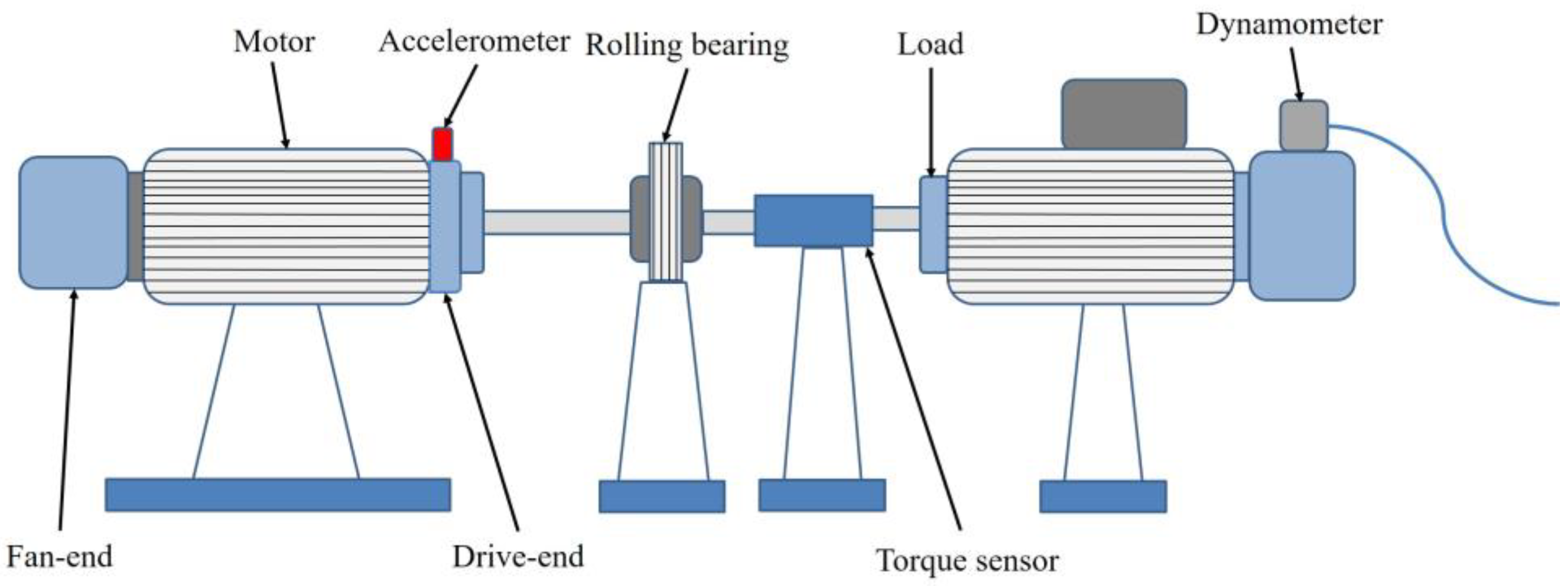
In this subsection, the experimental data of rolling bearings from the CWRU bearing failure simulation bench (shown in Figure 7) are used to test the effectiveness of the DAMGCN. The experimental conditions were set as follows: the signal sampling frequency was set to 12 kHz; the motor loads were 0 hp, 1 hp, 2 hp, and 3 hp; and their corresponding rotational speeds were 1797 rpm, 1772 rpm, 1750 rpm, and 1736 rpm, respectively. These four types of speed conditions were considered four different operating conditions, which were noted as 0, 1, 2, and 3. The vibration signals of the bearings were ascertained by the acceleration vibration sensors on the drive-end bearings for four different operating conditions, of which a total of three fault classes were possible: 0.007 mm (minor fault class), 0.014 mm (moderate fault class), and 0.021 mm (severe fault class). To summarize, a total of 10 health conditions of rolling bearings were selected for this experimental simulation, namely, rolling body minor failure (BS), outer ring minor failure (ORS), inner ring minor failure (IRS), rolling body moderate failure (BM), outer ring moderate failure (ORM), inner ring moderate failure (IRM), rolling body severe failure (BL), outer ring severe failure (ORL), inner ring severe failure (IRL), and normal condition (N). In this part of the experiment, the bearing data are first subjected to Z-score normalization, and then, the sliding window method is used to intercept the nonoverlapping vibration signals. Taking 1024 data as a sample, the training and test sets are divided into a ratio of 8:2. In the CWRU dataset, the total number of samples is 1600. Divided by 8:2, there are 1280 training samples and 320 test samples.

Table 1. Variable condition fault diagnosis task for the CWRU dataset.

Motor load (HP)	0	1	2	3
Rotational speeds (rpm)	1797	1772	1750	1730
Task	0	1	2	3

is the transfer diagnosis task table for the CWRU dataset.

For the CWRU bearing dataset, we establish 12 transfer fault diagnosis tasks to verify and analyze the superiority of the proposed method. For convenience, let ${\mathsf{\Gamma }}_{ab}$ represent the transfer task, $a\to b$, where $a$ represents the source domain with labeled data, and $b$ represents the target domain with unlabeled data. The DAMGCN model trains the labeled data in domain $a$ to accurately classify the unlabeled data in domain $b$. In the process of training, all data in $a$ and a small amount of data in $b$ will be input into the DAMGCN for training, and the remaining data in $b$ will be used only for testing. The structural parameters of DAMGCN are given in

Table 2. Detailed structural parameters of DAMGCN.

Component	Layer	Filter	Output Size
Spatial feature extractor (ResNet-18)	Input	/	64 × 1024
	1d Conv layer_1	16 × 7 × 1	64 × 16 × 512
	Pooling_1	3 × 1 max-pool	64 × 16 × 256
	Residual layer_1	32 × 3 × 1	64 × 16 × 256
	Residual layer_2	64 × 3 × 1	64 × 64 × 128
	Residual layer_3	128 × 3 × 1	64 × 128 × 64
	Residual layer_4	256 × 3 × 1	64 × 256 × 32
	Pooling_2	1 × 1 adaptive max-pool	64 × 256 × 1
Structural feature extractor (MGCN)	GGL	256 × 10	64 × 64
	MGConv_1	256 × 2000	64 × 2000
	MGConv_2	2000 × 500	64 × 500
	Linear layer_1	500 × 256	64 × 256
Classifier	Linear layer_2	256 × 10	64 × 10
Discriminator	Linear layer_3	256 × 256	64 × 256
	Linear layer_4	256 × 256	64 × 256
	Linear layer_5	256 × 1	64 × 1

.

In this experiment, to assess the performance and advantages of the developed methods, five different methods were used for comparative experiments, namely, baseline CNN, MK-MMD [39], joint maximum mean difference (JMMD) [40], DANN [34], and condition domain-adversarial neural network (CDANN) [35]. Distinguishing from the methods proposed in this paper, the feature extractors of the above five methods all use four-layer CNNs with the structural parameters shown in

Table 3. Detailed structural parameters of the four-layer CCN.

Component	Layer	Filter	Output Size
Spatial feature extractor (CNN)	Input	/	64 × 1024
	1d Conv layer_1	16 × 15 × 1	64 × 16 × 1010
	1d Conv layer_2	32 × 3 × 1	64 × 32 × 1008
	Pooling_2	2 × 1 max-pool	64 × 32 × 504
	1d Conv layer_3	64 × 3 × 1	64 × 64 × 502
	1d Conv layer_4	128 × 3 × 1	64 × 128 × 500
	Pooling_4	4 × 1 adaptive max-pool	64 × 128 × 4
	Linear layer_1	512 × 256	64 × 256

. MK-MMD is a representative method based on distance. On the basis of the CNN model, MK-MMD loss is used to minimize the difference in feature distribution between the source domain and target domain. Similarly, JMMD uses JMMD losses to minimize distribution differences. The network architecture of DANN is the same as that of MK-MMD and JMMD. The difference is that DANN only adds a domain classifier behind the feature extractor and relies on domain combat loss to achieve the same effect as the distance loss in the first two methods. CDANN is a further improvement on the basis of DANN. Compared with DANN, CDANN can capture complex multi-mode structures, adjust the domain discriminator more securely, and achieve a better data alignment effect.

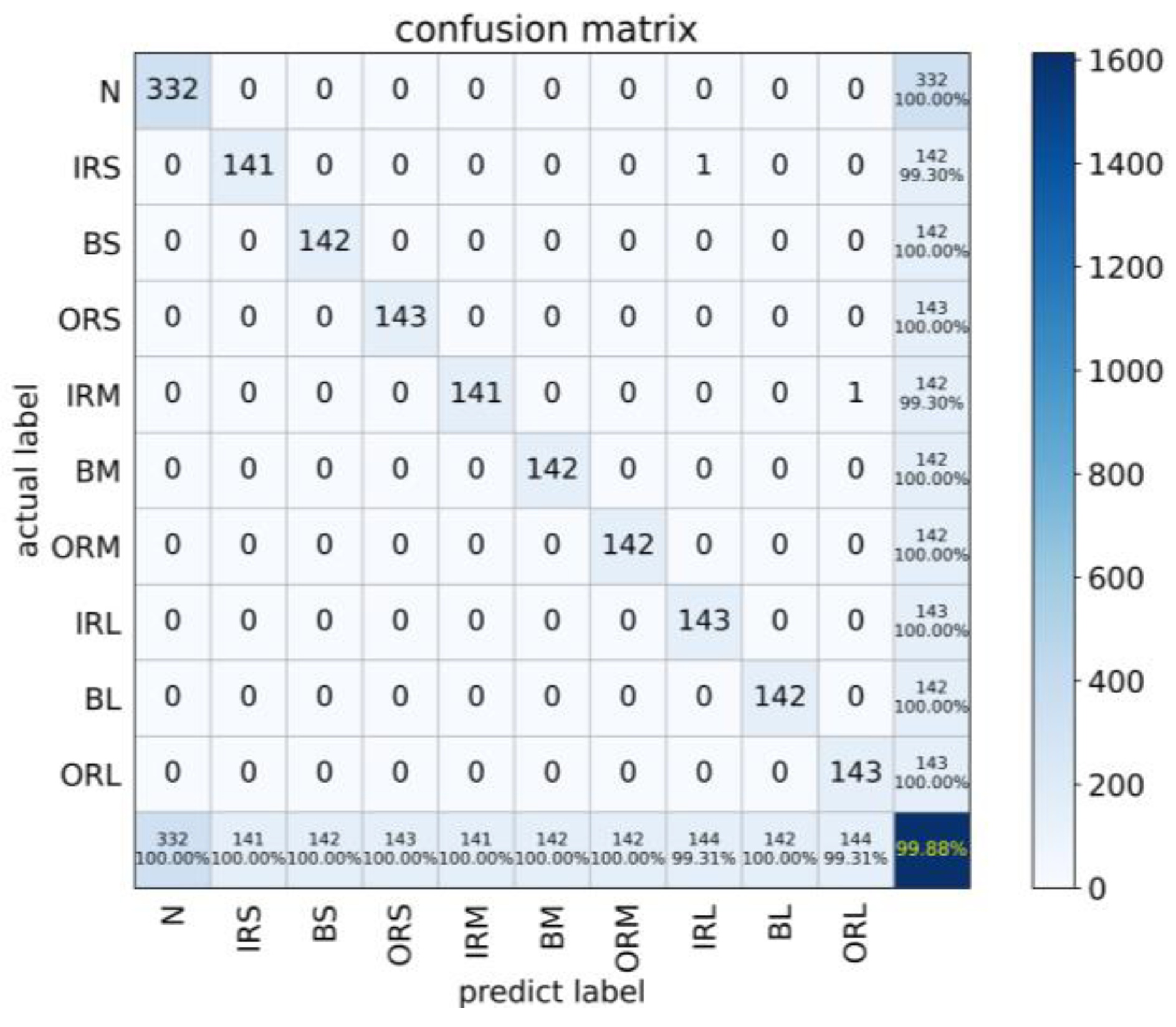
We knew the impact of the super parameter setting on the results, so we decided to set the model super parameters in the experimental part of this paper uniformly according to the super parameter setting in reference [20]. In addition, we also knew that the larger the epoch is, the more stable the model accuracy curve will be. However, in order to save computing resources, the training epoch is set as 100 in this paper, which can also meet the training requirements, as shown in Figure 7. All methods follow the following training parameter settings: the maximum number of epochs is 100, and the batch size is set to 64. The learning rate, $\eta$, is defined as 0.001, and it is decayed by multiplying by 0.1 at 50 and 75 epochs. The two trade-off parameters, $\alpha$ and $\beta$, in the total loss function, $L_{total}$, are calculated as $\left[1-\exp \left(-\tau \nu \right)\right]/\left[1+\exp \left(-\tau \nu \right)\right]$, where $\tau$ is 10 if the model is undergoing transfer learning training; $\nu$ is 0, and, if not, $\nu$ is 1. Taking the optional $0\to 1$ transfer task as an example, the accuracy and loss curve of the DAMGCN and its corresponding confusion matrix diagram are drawn to visualize the training loss of the DAMGCN to better observe the state of the model training process, as shown in Figure 8 and Figure 9.

From the above figure, we can know that the proposed DAMGCN can effectively complete the fault diagnosis task under variable working conditions. In Figure 9, we can clearly know that the accuracy and loss in the DAMGCN stabilize after about 45 epochs without wide fluctuations, and both the accuracy and loss achieve satisfactory results.

To better highlight the superiority of the DAMGCN, the following are the experimental results of six methods under twelve variable working condition fault diagnosis tasks. To decrease the randomness brought on by the model training, we set the total epoch in each transfer task to 100, took the average of the last 10 epoch results as the classification accuracy of 1 training period, and repeated 10 experiments to take the average of the results as the final classification accuracy. The diagnostic results of the six comparison methods are shown in

Table 4. Variable condition fault diagnosis task of JNU dataset.

Speed (rpm)	600	800	1000
Task	0	1	2

, and their corresponding histograms are shown in Figure 10.

According to the above results, for the twelve variable condition fault diagnosis tasks under the CWRU bearing dataset, the DAMGCN has good results compared to the rest of the fault diagnosis methods, both in simple cross-domain tasks (${\mathsf{\Gamma }}_{01}$, ${\mathsf{\Gamma }}_{02}$, ${\mathsf{\Gamma }}_{12}$, etc.) and in difficult cross-domain tasks (${\mathsf{\Gamma }}_{03}$, ${\mathsf{\Gamma }}_{13}$, ${\mathsf{\Gamma }}_{32}$, etc.). For example, in the simple transfer task, ${\mathsf{\Gamma }}_{02}$, the accuracy of the baseline CNN model with the worst classification performance reaches 98.56%, while the proposed DAMGCN accuracy is 100%, which can achieve perfect cross-domain fault classification. In the difficult transfer task, ${\mathsf{\Gamma }}_{31}$, the highest classification accuracy among the remaining five methods is 91.95%, while the classification accuracy of the DAMGCN method reaches 99.81%, which is an improvement of 7.86%, and its classification performance is also greatly improved. According to the above experimental results of the cross-domain tasks, the DAMGCN achieves good diagnosis results for different tasks with certain robustness, and the classification ability of the DAMGCN is also improved compared with other comparison methods, which indicates that the combination MGCN + ResNet-18 feature extractor also has stronger data feature mining capabilities than the basic four-layer CNN, which provides a subsequent high-precision fault classification effect, laying a solid foundation.

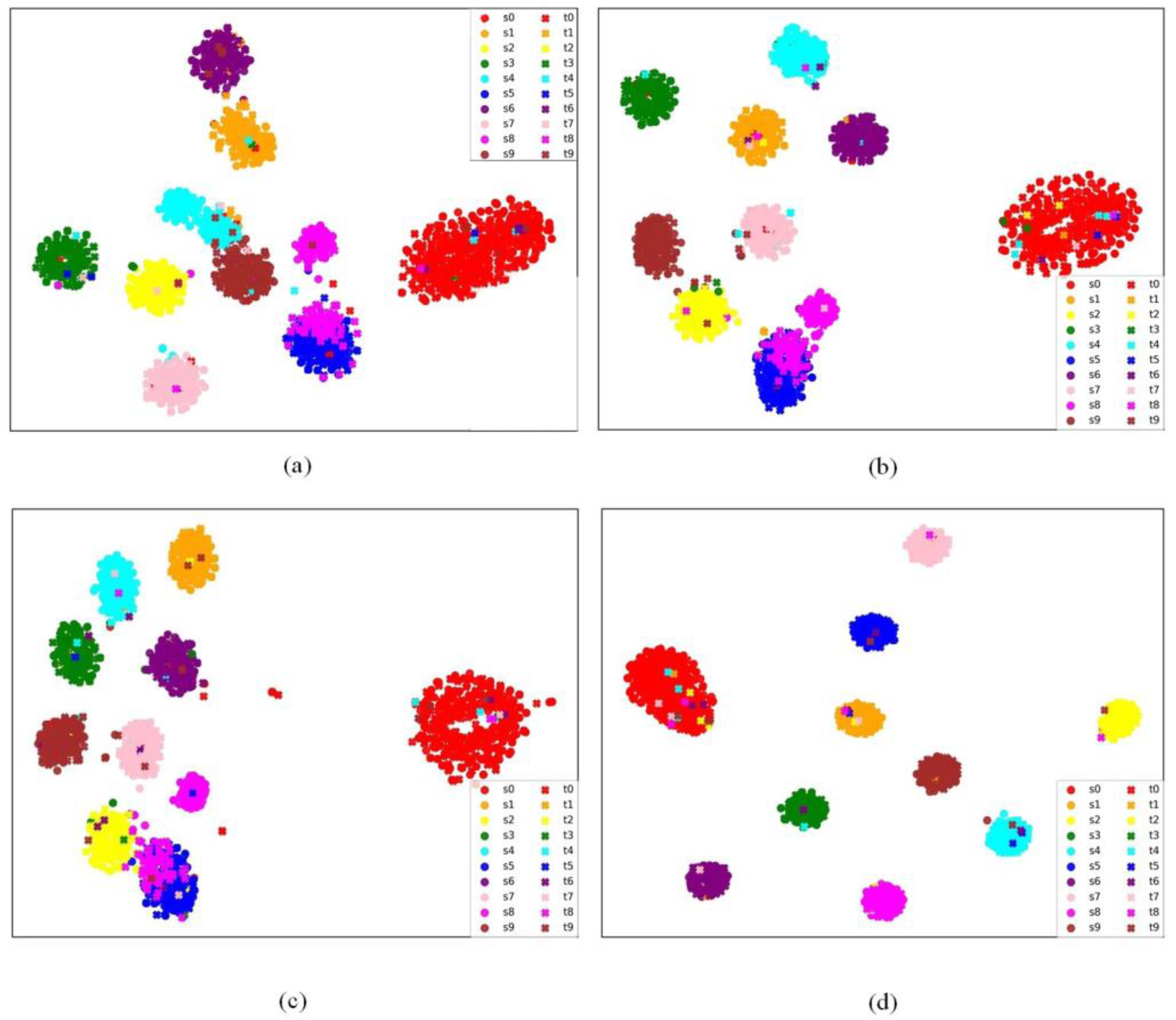
To verify the feature extraction ability of the proposed method, we now take the ${\mathsf{\Gamma }}_{03}$ transfer task as an example to supplement the T-SNE visualization of the baseline CNN, DANN, CDANN, and DAMGCN methods, as shown in Figure 11.

From Figure 11, we can clearly see that, compared with the other three methods, the feature extraction ability of the proposed DAMGCN model has been significantly improved, and the source domain features and target domain features can basically overlap effectively, which verifies the superiority of the method in feature clustering and feature extraction.

4.2. Case 2: JNU Failure Dataset

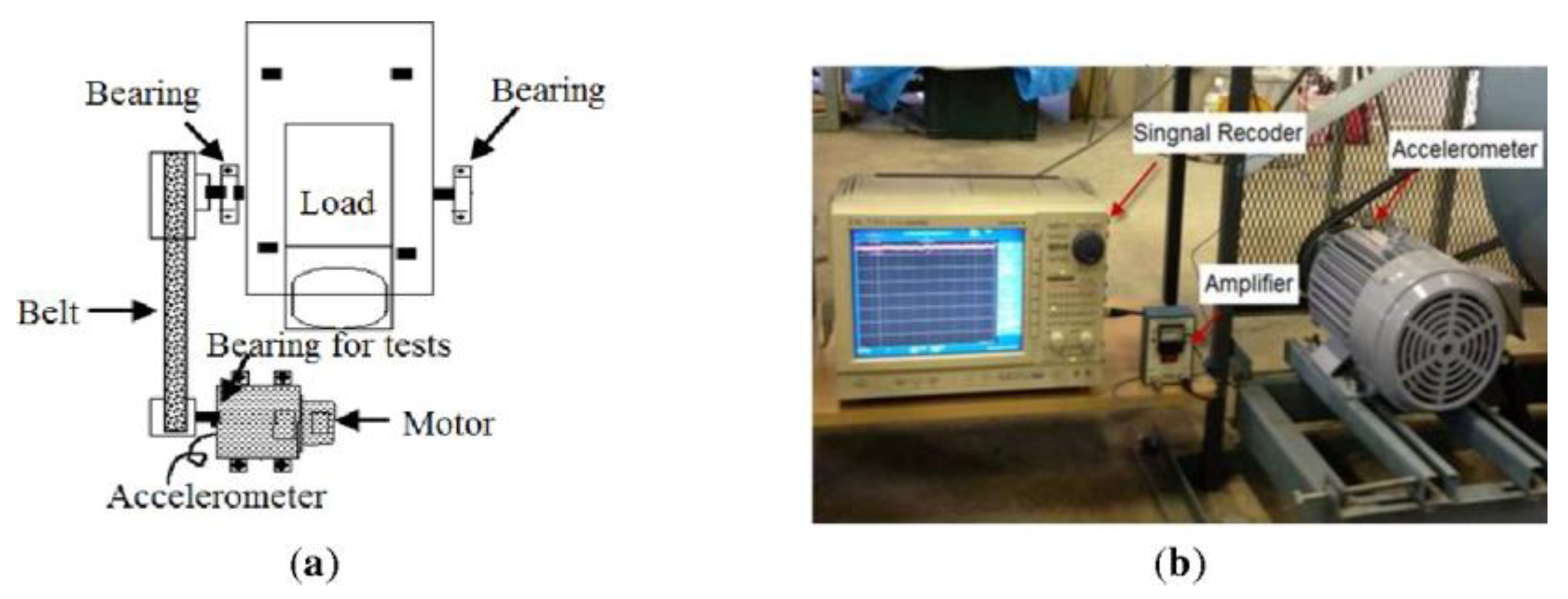
In this subsection, the bearing dataset from the JNU rolling bearing failure experimental bench (shown in Figure 12) is used to further verify the performance and applicability of the DAMGCN model. The basic conditions of this experimental bench are defined as follows: the sampling frequency is set to 50 kHz; the motor speed has three stages, 600 rpm, 800 rpm, and 1000 rpm; and, similarly, these three different speed conditions are considered three different operating conditions, which are noted as 0, 1, and 2. The raw signals of the experimental bearing, ER-12K, are obtained with the data acquisition instrument, and there are four health conditions: inner ring failure (IB), outer ring failure (OB), rolling element failure (TB), and normal condition (N), as shown in Figure 13, which is the three different failure conditions of the JNU rolling bearing. Similar to the CWRU dataset, in the JNU fault diagnosis experimental part, the bearing data are also normalized by a Z-score, each sample includes 1024 data, and the sliding window method is utilized to intercept the nonoverlapping sample set, and the training and testing sample sets are divided into a ratio of 8:2. In the JNU dataset, the total number of samples is 3500, divided by an 8:2 ratio, 2800 training samples, and 700 test samples.

Table 5. Experimental results of CWRU dataset (%).

Transfer Task	CNN	MK-MMD	JMMD	DANN	CDANN	DAMGCN
${\mathsf{\Gamma }}_{01}$	96.5 ± 2.4	97.1 ± 0.8	97.3 ± 1.2	96.4 ± 2.1	98.9 ± 1.5	99.4 ± 0.6
${\mathsf{\Gamma }}_{02}$	98.1 ± 1.9	98.8 ± 1.4	99.2 ± 0.6	99.4 ± 1.6	99.8 ± 1.3	100 ± 1.1
${\mathsf{\Gamma }}_{03}$	87.9 ± 1.3	90.4 ± 2.2	90.8 ± 1.5	89.6 ± 2.4	91.4 ± 1.9	99.1 ± 1.7
${\mathsf{\Gamma }}_{10}$	96.2 ± 0.8	98.1 ± 1.5	98.9 ± 1.1	99.4 ± 1.7	99.4 ± 0.8	99.8 ± 1.4
${\mathsf{\Gamma }}_{12}$	94.5 ± 2.6	100 ± 1.3	99.7 ± 2.6	98.3 ± 1.9	99.6 ± 1.4	100 ± 0.5
${\mathsf{\Gamma }}_{13}$	89.8 ± 1.4	94.9 ± 2.1	97.6 ± 1.5	97.2 ± 2.4	93.5 ± 1.6	99.4 ± 0.8
${\mathsf{\Gamma }}_{20}$	90.1 ± 1.7	98.2 ± 1.7	98.4 ± 1.1	98.5 ± 2.7	98.3 ± 0.7	99.5 ± 1.1
${\mathsf{\Gamma }}_{21}$	92.6 ± 2.2	98.4 ± 2.5	97.8 ± 1.7	97.4 ± 1.6	91.5 ± 1.1	99.4 ± 2.4
${\mathsf{\Gamma }}_{23}$	93.7 ± 1.8	96.7 ± 1.3	98.1 ± 2.4	95.4 ± 1.5	95.6 ± 2.8	99.5 ± 1.0
${\mathsf{\Gamma }}_{30}$	90.4 ± 2.4	96.5 ± 2.2	93.4 ± 1.3	91.1 ± 2.6	89.4 ± 1.4	98.6 ± 1.3
${\mathsf{\Gamma }}_{31}$	89.1 ± 1.2	90.8 ± 1.7	92.6 ± 1.2	93.4 ± 3.3	92.5 ± 2.3	99.8 ± 1.4
${\mathsf{\Gamma }}_{32}$	88.4 ± 0.8	95.3 ± 2.4	91.7 ± 2.2	93.8 ± 1.5	90.4 ± 1.7	99.4 ± 0.9
Average	92.3	96.3	96.3	95.8	95.0	99.4

shows cross-domain fault diagnosis tasks for the JNU dataset.

In the JNU experiments, six cross-domain fault diagnosis tasks are performed to analyze and compare the superiority and applicability of the DAMGCN in variable condition fault diagnosis. Similarly, for the convenience of representation, let $J_{ab}$ denote the transfer task, $a\to b$.

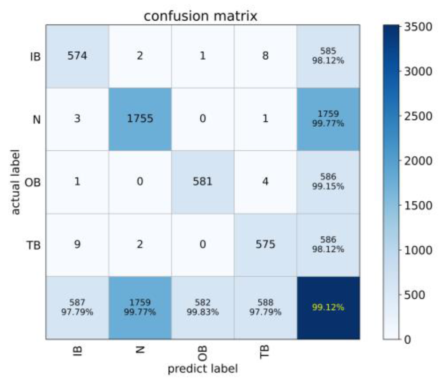
To validate the superiority and applicability of the DAMGCN method in the diagnosis of rolling bearing faults in different work conditions, Case 2 compares the proposed DAMGCN with the five different fault diagnosis methods in Section 2.1, where the basic parameters are kept the same as in Experiment 1. Firstly, the output confusion matrix, accuracy, and loss curves of the proposed DAMGCN under this transfer fault diagnosis task are visualized using the $0\to 1$ variable condition fault diagnosis task as an example, as shown in Figure 14 and Figure 15.

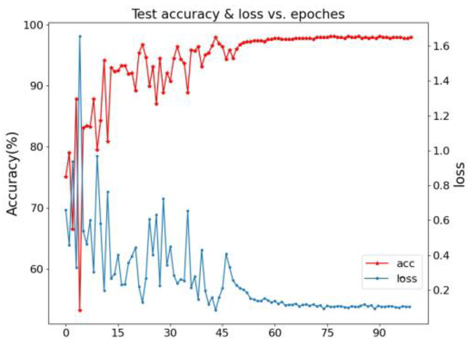
From the above figure, we can know that the proposed DAMGCN can still achieve valuable fault identification results for the four-classification transfer fault diagnosis task of the JNU dataset, reaching an accuracy of 99.12% under the $0\to 1$ variable operating condition task. In addition, the accuracy and loss curves of the test samples of the DAMGCN model show that the curve of the JNU dataset oscillates more obviously and fluctuates more greatly than that of the CWRU dataset within the first few tens of epochs, but after fifty epochs, the curve smooths out and converges well, achieving high accuracy and low loss, which demonstrates the effectiveness of the DAMGCN model.

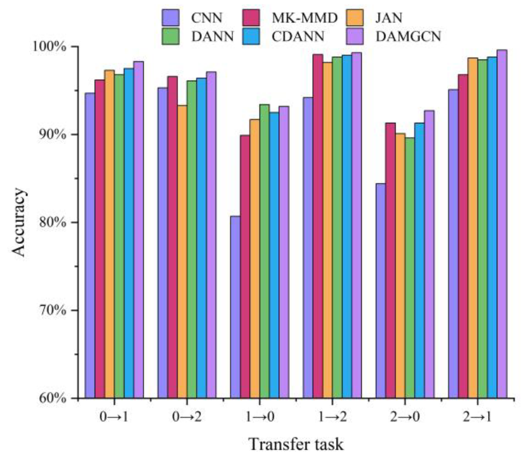
The following are the results of the comparison experiments of different fault diagnosis methods under six cross-domain tasks. The diagnostic results are shown in

Table 6. Experimental results of JNU dataset (%).

Transfer Task	CNN	MK-MMD	JMMD	DANN	CDANN	DAMGCN
$J_{01}$	94.7 ± 1.6	96.2 ± 2.1	97.3 ± 1.4	96.8 ± 2.3	97.5 ± 0.9	98.3 ± 1.3
$J_{02}$	95.3 ± 1.6	96.6 ± 1.2	93.3 ± 0.8	96.1 ± 1.7	96.4 ± 2.1	97.1 ± 1.2
$J_{10}$	80.7 ± 3.4	89.9 ± 1.4	91.7 ± 3.1	93.4 ± 0.8	92.5 ± 1.9	93.2 ± 2.2
$J_{12}$	94.2 ± 2.0	99.1 ± 1.7	98.2 ± 1.3	98.8 ± 2.6	99.0 ± 3.4	99.3 ± 3.1
$J_{20}$	84.4 ± 3.3	91.3 ± 2.7	90.1 ± 1.4	89.6 ± 1.9	91.3 ± 2.1	92.7 ± 1.6
$J_{21}$	95.1 ± 4.1	96.8 ± 1.5	98.7 ± 3.4	98.5 ± 0.8	98.8 ± 2.6	99.6 ± 0.8
Average	90.7	95.0	94.9	95.5	95.9	96.7

, and its corresponding histogram is shown in Figure 16.

According to the above figure, the proposed DAMGCN still obtains the best diagnostic accuracy in the transfer task of the JNU dataset, which is consistent with our previous test results in the CWRU dataset. Compared with the experimental results of the CWRU dataset, the classification performance of each method in the JNU dataset is degraded to some extent, and the high-accuracy fault identification, similar to that of the CWRU dataset, cannot be achieved, but DAMGCN still maintains the highest diagnostic accuracy, which indicates that the DAMGCN has higher robustness and adaptability compared with other methods. Furthermore, the average classification accuracy of DAMGCN is 96.56% in six cross-domain fault diagnosis tasks, which makes DAMGCN competent for different variable fault diagnosis tasks, and it achieves a more stable and accurate classification target than other fault diagnosis methods. The above results further prove the superiority and robustness of DAMGCN in the cross-domain task, which is of high value for practical engineering applications.

Compared with the existing domain adaptation methods, the DAMGCN proposed in this paper can obtain the node information in different receptive fields and the local node information in the same receptive field by relying on the unique three-layer graph convolution layer architecture and fully mining the data structure information, while the GATConv layer can realize the adaptive matching of the weights of different adjacent nodes. According to the above experimental results, the proposed model has higher accuracy and stronger generalization.

4.3. Ablation Experiments

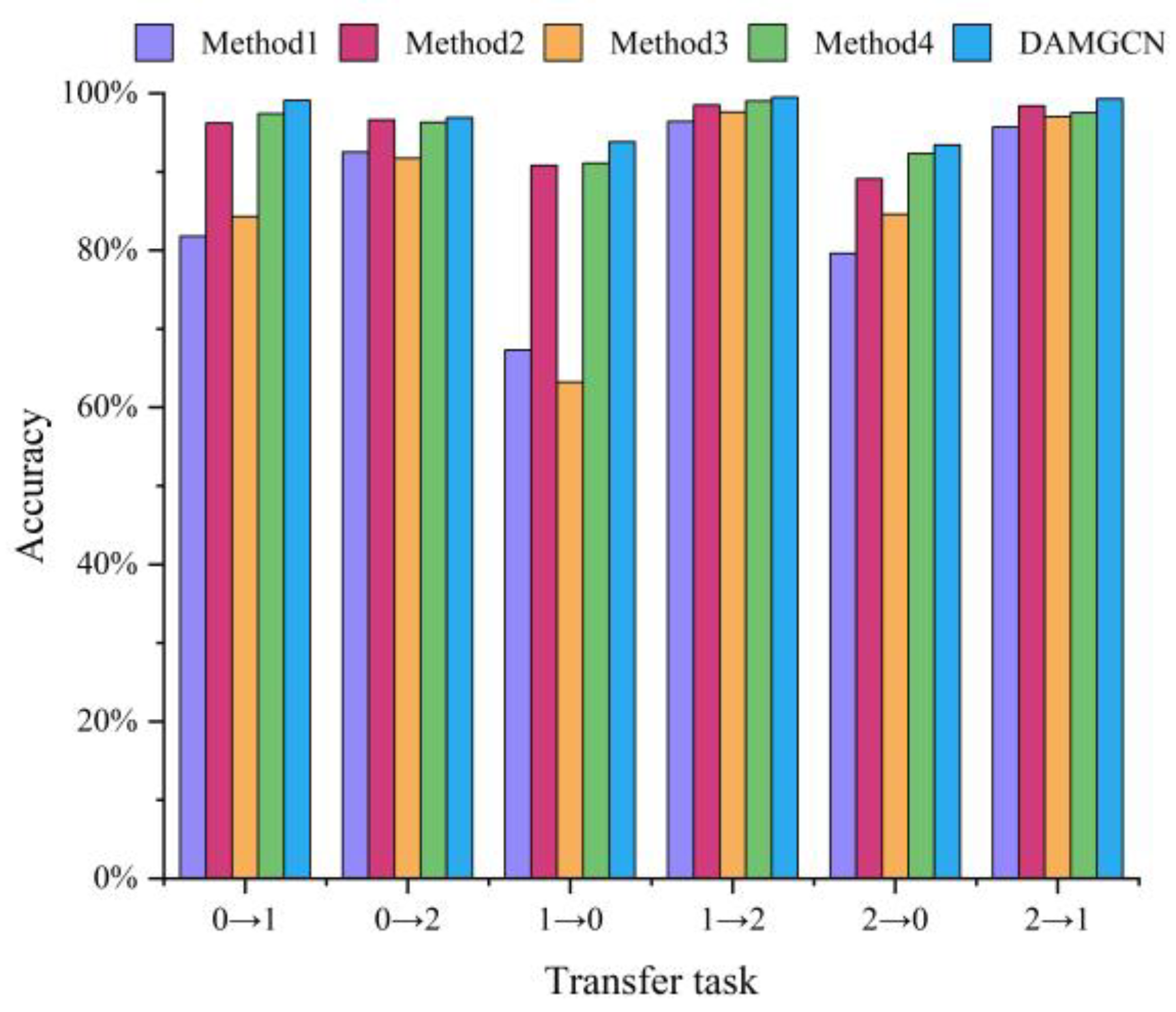
For the sake of distinguishing the impact of each individual section of the DAMGCN on the model function, an ablation experiment is conducted to discuss this issue. Four variant methods are further derived from the DAMGCN: (1) Method1 (no domain confrontation), (2) Method2 (no structural alignment loss), (3) Method3 (both no domain confrontation and no structural alignment loss), and (4) Method4 (no MGCN feature extractor). The experimental results of the four variant methods and the DAMCCN for the transfer task on the JNU dataset are provided in

Table 7. Results of ablation experiments on JNU dataset (%).

Transfer Task	Method1	Method2	Method3	Method4	DAMGCN
$J_{01}$	81.8 ± 1.9	96.2 ± 2.4	84.3 ± 2.6	97.4 ± 1.8	99.1 ± 2.2
$J_{02}$	92.5 ± 3.2	96.6 ± 2.5	91.7 ± 3.3	96.3 ± 1.5	96.9 ± 0.5
$J_{10}$	67.3 ± 2.7	90.8 ± 1.6	63.2 ± 2.1	91.1 ± 2.6	93.8 ± 1.4
$J_{12}$	96.4 ± 1.3	98.5 ± 1.1	97.6 ± 2.4	99.0 ± 0.8	99.5 ± 1.2
$J_{20}$	79.6 ± 3.8	89.1 ± 2.2	84.6 ± 1.5	92.3 ± 2.2	93.4 ± 1.6
$J_{21}$	95.7 ± 1.8	98.4 ± 1.4	97.0 ± 2.7	97.5 ± 1.6	99.3 ± 0.7
Average	85.6	94.9	86.4	95.6	97.0

, and the corresponding histograms are shown in Figure 17.

According to the above results, we can know that the final classification accuracy of the DAMGCN is improved to different degrees compared with the four variants. This fully illustrates that all three components—domain confrontation, structural feature alignment, and MGCN data structure feature extractor—play an absolutely necessary role in the classification effect of the model, which can heighten the cross-domain fault diagnosis ability of the model.

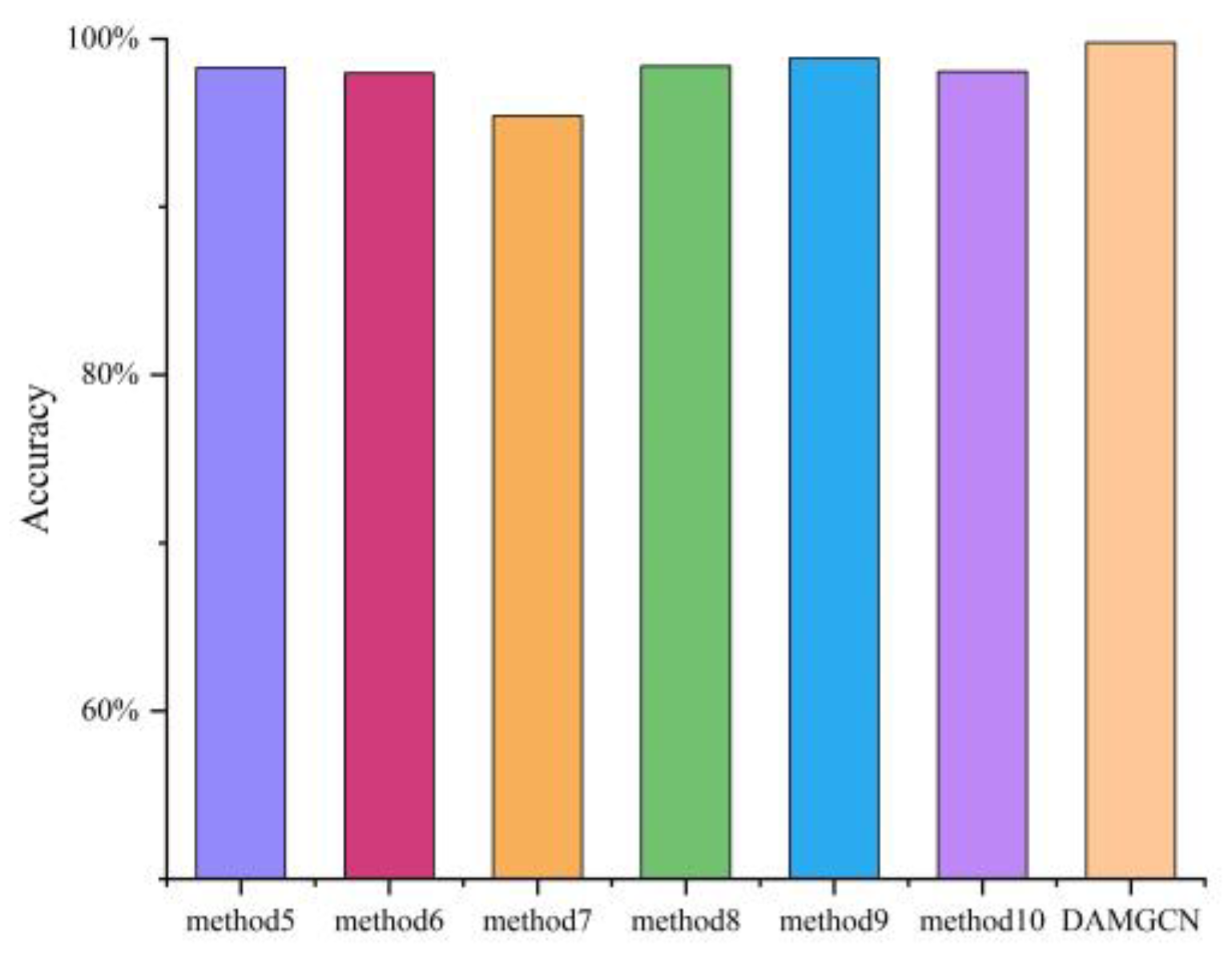
In order to fully explain the impact of different convolution layers on the model performance, we conducted comparative tests on models with different convolutional layers. The details are as follows: (1) Method5 (only MRFConv), (2) Method6 (only LEConv), (3) Method7 (only GATConv), (4) Method 8 (MRFConv + LEConv), (5) Method9 (MRFConv + GATConv), and (6) Method10 (LEConv + MRFConv). The above six methods and the classification accuracy of the proposed DAMGCN under transfer task ${\mathsf{\Gamma }}_{12}$ are shown in Figure 18.

It can be seen from Figure 18 that, compared with other methods, DAMGCN benefits from the joint action of three different graph convolutional layers and achieves the best fault classification effect.

4.4. Noise Experiment

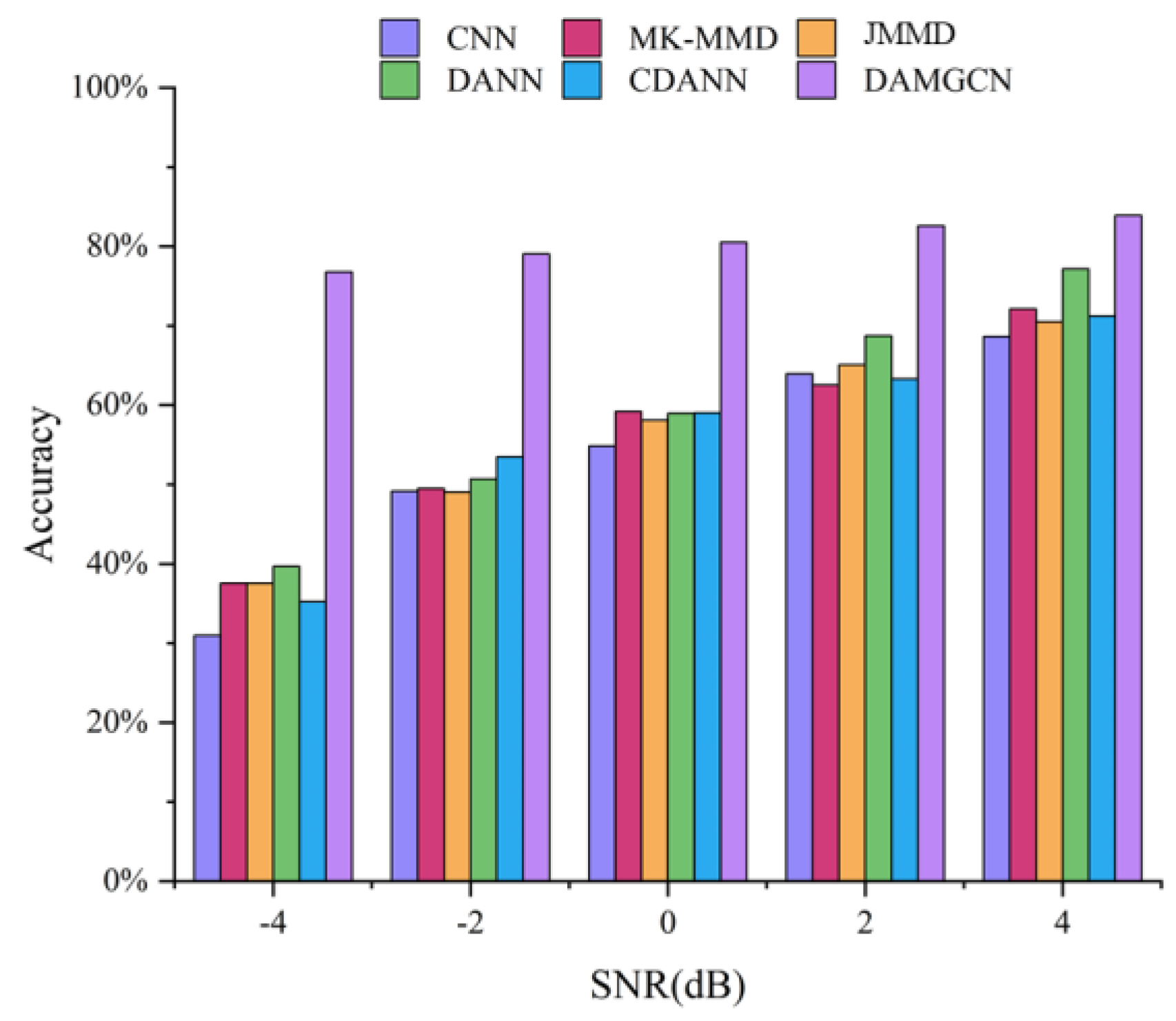
We added −4, −2, 0, 2, and 4 dB white Gaussian noise values to the CWRU dataset and then tested the above different noisy datasets on transfer task ${\mathsf{\Gamma }}_{12}$ using the proposed DAMGCN model. The results are shown in Figure 19.

It can be seen from the above figure that the proposed method can achieve good fault classification accuracy under different signal-to-noise ratios (SNR). Compared with other methods, it has better resistance to noise environments, which further verifies that DAMGCN has a great noise-resistance effect. We think the main reasons are as follows: (1) The proposed MGCN takes into account the global node information of different receptive fields and local node information around the node and aggregates the node information into a feature representation with a larger amount of information. (2) The GATConv layer is used to judge the importance of different node information and filter out useless node information, which naturally includes interference information such as noise. Therefore, a more accurate fault diagnosis effect can be achieved under noise conditions.

5. Conclusions

To further improve the feature learning, as well as classification capability, of traditional cross-domain fault diagnosis models, a novel and efficient model (DAMGCN) for UDA is proposed in this paper. The DAMGCN can more validly achieve the alignment of class labels, domain labels, and data structures by fusing four major components: a spatial feature extractor, a structural feature extractor, a domain discriminator, and a structural alignment block. The results of two cross-domain fault diagnosis comparison experiments also show that the proposed DAMGCN has better robustness and applicability and can achieve higher classification accuracy than other comparison methods, which verifies the effectiveness and applicability of DAMGCN for the fault diagnosis of rolling bearings under variable working conditions. In addition, ablation experiments and noise experiments also verify the robustness and generalization of the proposed DAMGCN under the influence of model construction and noisy conditions. In conclusion, the proposed DAMGCN has achieved satisfactory results in the field of UDA fault diagnosis, which can serve as a reference for future research work.

References

1. Su, H.; Xiang, L.; Hu, A.; Xu, Y.; Yang, X. A novel method based on meta-learning for bearing fault diagnosis with small sample learning under different working conditions. Mech. Syst. Signal Process. 2022, 169, 108765. [Google Scholar] [CrossRef]
2. Liao, Y.; Huang, R.; Li, J.; Chen, Z.; Li, W. Deep Semi-supervised Domain Generalization Network for Rotary Machinery Fault Diagnosis under Variable Speed. IEEE Trans. Instrum. Meas. 2020, 69, 8064–8075. [Google Scholar] [CrossRef]
3. Huang, R.; Li, J.; Wang, S.; Li, G.; Li, W. A Robust Weight-Shared Capsule Network for Intelligent Machinery Fault Diagnosis. IEEE Trans. Ind. Inform. 2020, 16, 6466–6475. [Google Scholar] [CrossRef]
4. Lee, J.; Kim, M.; Ko, J.U.; Jung, J.H.; Sun, K.H.; Youn, B.D. Asymmetric inter-intra domain alignments (AIIDA) method for intelligent fault diagnosis of rotating machinery. Reliab. Eng. Syst. Saf. 2021, 218, 108186. [Google Scholar] [CrossRef]
5. Qiu, H.; Lee, J.; Lin, J.; Yu, G. Wavelet filter-based weak signature detection method and its application on rolling element bearing prognostics. J. Sound Vib. 2006, 289, 1066–1090. [Google Scholar] [CrossRef]
6. Yuan, J.; Zhao, R.; He, T.; Chen, P.; Wei, K.; Xing, Z. Fault diagnosis of rotor based on Semi-supervised Multi-Graph Joint Embedding. ISA Trans. 2022. [Google Scholar] [CrossRef]
7. Bishop, C.M.; Nasrabadi, N.M. Pattern Recognition and Machine Learning; Springer: New York, NY, USA, 2006. [Google Scholar]
8. Li, X.; Jia, X.; Zhang, W.; Ma, H.; Luo, Z.; Li, X. Intelligent cross-machine fault diagnosis approach with deep auto-encoder and domain adaptation. Neurocomputing 2019, 383, 235–247. [Google Scholar] [CrossRef]
9. Zhao, Z.; Wu, S.; Qiao, B.; Wang, S.; Chen, X. Enhanced Sparse Period-Group Lasso for Bearing Fault Diagnosis. IEEE Trans. Ind. Electron. 2018, 66, 2143–2153. [Google Scholar] [CrossRef]
10. Lei, Y.; Jia, F.; Lin, J.; Xing, S.; Ding, S.X. An Intelligent Fault Diagnosis Method Using Unsupervised Feature Learning Towards Mechanical Big Data. IEEE Trans. Ind. Electron. 2016, 63, 3137–3147. [Google Scholar] [CrossRef]
11. LeCun, Y.; Bengio, Y.; Hinton, G. Deep learning. Nature 2015, 521, 436–444. [Google Scholar] [CrossRef]
12. Khan, S.; Yairi, T. A review on the application of deep learning in system health management. Mech. Syst. Signal Process. 2018, 107, 241–265. [Google Scholar] [CrossRef]
13. Cheng, Y.; Lin, M.; Wu, J.; Zhu, H.; Shao, X. Intelligent fault diagnosis of rotating machinery based on continuous wavelet transform-local binary convolutional neural network. Knowl. -Based Syst. 2021, 216, 106796. [Google Scholar] [CrossRef]
14. Zhao, X.; Jia, M. A new Local-Global Deep Neural Network and its application in rotating machinery fault diagnosis. Neurocomputing 2019, 366, 215–233. [Google Scholar] [CrossRef]
15. Liu, W.; Guo, P.; Ye, L. A Low-Delay Lightweight Recurrent Neural Network (LLRNN) for Rotating Machinery Fault Diagnosis. Sensors 2019, 19, 3109. [Google Scholar] [CrossRef] [Green Version]
16. Shi, J.; He, Q.; Wang, Z. An LSTM-based severity evaluation method for intermittent open faults of an electrical connector under a shock test. Measurement 2020, 173, 108653. [Google Scholar] [CrossRef]
17. Jiao, J.; Zhao, M.; Lin, J.; Ding, C. Classifier Inconsistency-Based Domain Adaptation Network for Partial Transfer Intelligent Diagnosis. IEEE Trans. Ind. Inform. 2019, 16, 5965–5974. [Google Scholar] [CrossRef]
18. Zhu, J.; Chen, N.; Shen, C. A New Deep Transfer Learning Method for Bearing Fault Diagnosis Under Different Working Conditions. IEEE Sens. J. 2019, 20, 8394–8402. [Google Scholar] [CrossRef]
19. Gopalan, R.; Li, R.; Chellappa, R. Unsupervised adaptation across domain shifts by generating intermediate data representations. IEEE Trans. Pattern Anal. Mach. Intell. 2014, 36, 2288–2302. [Google Scholar] [CrossRef]
20. Zhao, Z.; Zhang, Q.; Yu, X.; Sun, C.; Wang, S.; Yan, R.; Chen, X. Unsupervised deep transfer learning for intelligent fault diagnosis: An open source and comparative study. IEEE Trans. Instrum. Meas. 2021, 70, 3525828. [Google Scholar] [CrossRef]
21. Deng, M.; Deng, A.; Zhu, J.; Shi, Y.; Liu, Y. Intelligent fault diagnosis of rotating components in the absence of fault data: A transfer-based approach. Measurement 2020, 173, 108601. [Google Scholar] [CrossRef]
22. Wang, Y.; Sun, X.; Li, J.; Yang, Y. Intelligent Fault Diagnosis with Deep Adversarial Domain Adaptation. IEEE Trans. Instrum. Meas. 2020, 70, 1–9. [Google Scholar] [CrossRef]
23. Che, C.; Wang, H.; Ni, X.; Fu, Q. Domain adaptive deep belief network for rolling bearing fault diagnosis. Comput. Ind. Eng. 2020, 143, 106427. [Google Scholar] [CrossRef]
24. Li, T.; Zhao, Z.; Sun, C.; Yan, R.; Chen, X. Domain Adversarial Graph Convolutional Network for Fault Diagnosis Under Variable Working Conditions. IEEE Trans. Instrum. Meas. 2021, 70, 1–10. [Google Scholar] [CrossRef]
25. Wu, Z.; Pan, S.; Chen, F.; Long, G.; Zhang, C.; Yu, P.S. A comprehensive survey on graph neural networks. IEEE Trans. Neural. Networks Learn. Syst. 2020, 32, 4–24. [Google Scholar] [CrossRef] [PubMed] [Green Version]
26. Wu, Z.; Pan, S.; Long, G.; Jiang, J.; Zhang, C. Graph wavenet for deep spatial-temporal graph modeling. arXiv 2019, arXiv:1906.00121. [Google Scholar]
27. Li, T.; Zhao, Z.; Sun, C.; Yan, R.; Chen, X. Multi-receptive field graph convolutional networks for machine fault diagnosis. IEEE Trans. Ind. Electron. 2020, 68, 12739–12749. [Google Scholar]
28. Yang, C.; Zhou, K.; Liu, J. SuperGraph: Spatial-Temporal Graph-Based Feature Extraction for Rotating Machinery Diagnosis. IEEE Trans. Ind. Electron. 2021, 69, 4167–4176. [Google Scholar] [CrossRef]
29. Ranjan, E.; Sanyal, S.; Talukdar, P. ASAP: Adaptive Structure Aware Pooling for Learning Hierarchical Graph Representations. arXiv 2020, arXiv:1911.07979. [Google Scholar] [CrossRef]
30. Velikovi, P.; Cucurull, G.; Casanova, A.; Romero, A.; Liò, P.; Bengio, Y. Graph Attention Networks. arXiv 2017, arXiv:1710.10903. [Google Scholar]
31. Sun, B.; Saenko, K. Deep CORAL: Correlation Alignment for Deep Domain Adaptation; ECCV: Amsterdam, The Netherlands, 2016; pp. 443–450. [Google Scholar]
32. Sejdinovic, D.; Sriperumbudur, B.; Gretton, A.; Fukumizu, K. Equivalence of distance-based and RKHS-based statistics in hypoth-esis testing. Ann. Statist. 2013, 41, 2263–2291. [Google Scholar] [CrossRef]
33. Gretton, A.; Sejdinovic, D.; Strathmann, H.; Balakrishnan, S.; Pontil, M.; Fukumizu, K.; Sriperumbudur, B.K. Optimal kernel choice for large-scale two-sample tests. In Advances in Neural Information Processing Systems 25; MIT Press: Cambridge, MA, USA, 2012; pp. 1205–1213. [Google Scholar]
34. Ganin, Y.; Ustinova, E.; Ajakan, H.; Germain, P.; Larochelle, H.; Laviolette, F.; Marchand, M.; Lempitsky, V. Domain-Adversarial Training of Neural Networks. J. Mach. Learn. Res. 2016, 17, 2096-2030. [Google Scholar] [CrossRef] [Green Version]
35. Long, M.; Cao, Z.; Wang, J.; Jordan, M.I. Conditional adversarial domain adaptation. In Advances in Neural Information Processing Systems 31; MIT Press: Montreal, QC, Canada, 2018; pp. 1640–1650. [Google Scholar]
36. Hammond, D.K.; Vandergheynst, P.; Gribonval, R. Wavelets on graphs via spectral graph theory. Appl. Comput. Harmon. Anal. 2011, 30, 129–150. [Google Scholar] [CrossRef] [Green Version]
37. The Case Western Reserve University Bearing Data Center Website. Available online: https://engineering.case.edu/bearingdatacenter (accessed on 14 August 2022).
38. Li, K.; Ping, X.; Wang, H.; Chen, P.; Cao, Y. Sequential Fuzzy Diagnosis Method for Motor Roller Bearing in Variable Operating Conditions Based on Vibration Analysis. Sensors 2013, 13, 8013–8041. [Google Scholar] [CrossRef] [PubMed]
39. Long, M.; Cao, Y.; Cao, Z.; Wang, J.; Jordan, M.I. Transferable Representation Learning with Deep Adaptation Networks. IEEE Trans. Pattern Anal. Mach. Intell. 2018, 41, 3071–3085. [Google Scholar] [CrossRef] [PubMed]
40. Long, M.; Cao, Y.; Wang, J.; Jordan, M.I. Deep transfer learning with joint adaptation networks. In Proceedings of the International Conference on Machine Learning, Sydney, Australia, 6–11 August 2017; pp. 2208–2217. [Google Scholar] [CrossRef]
Figure 1. Schematic diagram of graph convolution network structure.
Symmetry 14 02654 g001
Figure 2. MGCN structure diagram.
Symmetry 14 02654 g002
Figure 3. LEConv operation diagram.
Symmetry 14 02654 g003
Figure 4. DAMGCN network architecture diagram.
Symmetry 14 02654 g004
Figure 5. The process of constructing an MGCN graph.
Symmetry 14 02654 g005
Figure 6. Flow chart of the DAMGCN fault diagnosis method in variable working conditions.
Symmetry 14 02654 g006
Figure 7. CWRU bearing failure simulation test bench.
Symmetry 14 02654 g007
Figure 8. Confusion matrix of transfer task Γ 01 for the CWRU dataset.
Symmetry 14 02654 g008
Figure 9. Accuracy and loss curve of transfer task Γ 01 for CWRU dataset.
Symmetry 14 02654 g009
Figure 10. Experimental results of CWRU dataset transfer task.
Symmetry 14 02654 g010
Figure 11. Feature visualization via T-SNE of transfer task Γ 03 . (a) CNN, (b) DANN, (c) CDANN, (d) DAMGCN.
Symmetry 14 02654 g011
Figure 12. JNU bearing failure simulation test bench. (a) Illustration of the rotation machinery, (b) Illustration of the motor in the field [38].
Symmetry 14 02654 g012
Figure 13. Three different failure states of JNU bearings. (a) outer-race defect, (b) inner-race defect, and (c) roller element defect [38].
Symmetry 14 02654 g013
Figure 14. Confusion matrix of transfer task Γ 01 for the JNU dataset.
Symmetry 14 02654 g014
Figure 15. Accuracy and loss curve of transfer task Γ 01 for JNU dataset.
Symmetry 14 02654 g015
Figure 16. Experimental results of JNU dataset transfer task.
Symmetry 14 02654 g016
Figure 17. Experimental results of the ablation of the JNU dataset migration fault diagnosis task.
Symmetry 14 02654 g017
Figure 18. Accuracy under different graph convolutional layers.
Symmetry 14 02654 g018
Figure 19. Accuracy under different SNR conditions.
Symmetry 14 02654 g019