Some New Optical Solitons of the Generalized Radhakrishnan–Kundu–Lakshmanan Equations with Powers of Nonlinearity

Abstract

In this paper, the new generalized Radhakrishnan–Kundu–Lakshmanan equations with powers of nonlinearity are studied, which is one of the important mathematical models in nonlinear optics. Using the complex envelope traveling wave solution, the new generalized Radhakrishnan–Kundu–Lakshmanan equations are transformed into the nonlinear systems of ordinary differential equations. Under certain constraint conditions, the obtained equations are transformed into a special nonlinear equation. With the help of the solution of this nonlinear equation, some new optical solutions of the new generalized Radhakrishnan–Kundu–Lakshmanan equations with powers of nonlinearity are obtained, which include the solitary wave, singular soliton, periodic soliton, singular-periodic soliton, and exponential-type soliton. By numerical simulation, the corresponding graphs of the optical soliton solution of the new generalized Radhakrishnan–Kundu–Lakshmanan equations are given under the given fixed parameter values, which include the 3D graphics of the module and the 3D graphics of the imaginary part. By analyzing the 2D graphics of the module changing with n, the amplitude of the wave is symmetrical or asymmetrical.

1. Introduction

Nonlinear partial differential equations (NPDEs) play a pivotal role in many areas, which can represent many nonlinear phenomena in many fields such as micro-physics, fluid flows, biology, chemistry, and other areas of engineering. The Radhakrishnan–Kundu–Lakshmanan equation is one of the important mathematical models in nonlinear optics, which has been widely concerned in recent years [1,2,3,4,5,6,7,8,9,10,11,12,13,14,15,16,17,18,19]. The Radhakrishnan–Kundu–Lakshmanan equation has many different forms.

The propagation of optical solitons in optical fibers has attracted much attention in the past few decades. Optical solitons are a type of solitary wave, which has the ability of wave propagation and will not spread over a long distance. Optical solitons are important in nonlinear optics because they are the fundamental key of telecommunications. Based on the role of solitons in communication links, optical pulse compressors, optical fibers, amplifiers, and other aspects, soliton mathematical models are very useful. Therefore, it is worthwhile to study the Radhakrishnan–Kundu–Lakshmanan equations and solve the optical solitons. Some effective methods have been proposed to find the optical soliton solutions, such as the Bäcklund transform method [20,21,22], the soliton ansatz method [23,24,25], the auxiliary equation method [26,27,28], the Lie group theory method [29,30], and so on. These methods of finding soliton solutions are also extended to fractional differential equations [31,32], which appear more and more frequently in different research fields.

Recently, novel generalized Radhakrishnan–Kundu–Lakshmanan equations with powers of nonlinearity were derived by N.A. Kudryashov in [10], and the form is as follows:

$$\begin{array}{c}\hfill i{q}_t+\lambda q_{xx}+{a\left|q\right|}^{n}q+{b\left|q\right|}^{2n}q+{c\left|q\right|}^{3n}q+{d\left|q\right|}^{4n}q={i\left(\alpha \right|q|}^{n}q+{\beta \left|q\right|}^{2n}q+{\gamma \left|q\right|}^{3n}q+{\delta \left|q\right|}^{4n}{q)}_x-i\chi q_{xxx},\end{array}$$

(1)

where $q(x,t)$ is the complex-valued function, which originates from waves, whilst x and t are spatial and temporal variables, respectively. $\lambda$ and $\chi$ are the real constant coefficients, representing the group velocity dispersion and third-order dispersion, respectively. The real constant coefficients $a,b,c,d,\alpha ,\beta ,\gamma ,\delta$ arise from the self-phase modulation effect, whereas n is a positive integer, and $i^2=-1$.

The exact solutions of Equation (1) were found in the form of implicit functions by the direct and special methods in [10]. The obtained solutions can be regarded as dark solitons and bright solitons. Equation (1) with $a=\alpha ,b=\beta ,c=\gamma ,d=\delta$ was studied by A.M. Alshehri et al. in [13]. The authors explored the conservation law of the equation and gave the conservation quantities expressed by special functions.

For Equation (1), it is difficult to find the exact solution. In this paper, the special case of Equation (1) is considered in the following form:

$$\begin{array}{c}\hfill i{q}_t+\lambda q_{xx}+{b\left|q\right|}^{2n}q+{d\left|q\right|}^{4n}q={i\left(\beta \right|q|}^{2n}q+{\delta \left|q\right|}^{4n}{q)}_x-i\chi q_{xxx}.\end{array}$$

(2)

The rest of this paper is arranged as follows. In Section 2, we give the mathematical analysis of Equation (2). In Section 3, we give analytical soliton solutions for Equation (2) by the auxiliary equation method. In Section 4, the wave structure is analyzed by graphical representations of the solution. Some conclusions are provided at the end of the paper.

2. Mathematical Analysis of Equation (2)

Suppose that the form of the complex envelope traveling wave solution of Equation (2) is

$$\begin{array}{c}\hfill q(x,t)=U\left(\xi \right)exp\left(i\mathsf{\Phi }(x,t)\right),\xi =\eta (x-\nu t),\mathsf{\Phi }=-kx+\omega t+{\theta }_0\end{array}$$

(3)

where $k,\nu ,\omega ,\eta$, and ${\theta }_0$ are the wave number, velocity, frequency, width, and phase constant of the soliton, respectively.

Substituting Equation (3) into Equation (2) and separating the imaginary and the real components yield the following nonlinear systems of ordinary differential equations:

$$\begin{array}{c}\hfill \chi U^{‴}-(\nu +2\lambda k+3\chi k^2)U^{\prime }-\beta (2n+1)U^{2n}{U}^{\prime }-\delta (4n+1)U^{4n}{U}^{\prime }=0,\end{array}$$

(4)

and

$$\begin{array}{c}\hfill (\lambda {\eta }^2-3\chi k{\eta }^2)U^{″}-(\omega +k^2\lambda +k^3\chi )U+(b-k\beta )U^{2n+1}+(d-\delta k)U^{4n+1}=0.\end{array}$$

(5)

Integrating Equation (4) and ignoring the integration constant, we derive the following equation:

$$\begin{array}{c}\hfill \chi U^{″}-(\nu +2\lambda k+3\chi k^2)U-\beta U^{2n+1}-\delta U^{4n+1}=0.\end{array}$$

(6)

As the function $U\left(\xi \right)$ satisfies Equations (4) and (6), we can give the following relation:

$$\begin{array}{c}\hfill \frac{\lambda {\eta }^2-3\chi k{\eta }^2}{\chi }=\frac{\omega +k^2\lambda +k^3\chi }{\nu +2\lambda k+3\chi k^2}=\frac{b-k\beta }{-\delta }=\frac{d-\delta k}{-\delta }.\end{array}$$

(7)

Now, Equation (6) is analyzed under the constraint conditions (7).

3. Analytical Soliton Solutions for Equation (2) by the Auxiliary Equation

Multiplying both sides of Equation (6) by $U^{\prime }$ and integrating once with respect to $\xi$, we obtain

$$\begin{array}{c}\hfill {\left(U^{\prime }\right)}^2-\frac{\nu +2\lambda k+3\chi k^2}{\chi }{U}^2-\frac{\beta }{(n+1)\chi }{U}^{2n+2}-\frac{\delta }{(2n+1)\chi }{U}^{4n+2}=C_0,\end{array}$$

(8)

where $C_0$ is the integral constant. Letting the integral constant be zero of Equation (8), we have the following auxiliary ordinary differential equation:

$$\begin{array}{c}\hfill {\left(U^{\prime }\right)}^2-\frac{\nu +2\lambda k+3\chi k^2}{\chi }{U}^2-\frac{\beta }{(n+1)\chi }{U}^{2n+2}-\frac{\delta }{(2n+1)\chi }{U}^{4n+2}=0.\end{array}$$

(9)

Letting

$$A=-\frac{\nu +2\lambda k+3\chi k^2}{\chi },B=-\frac{\beta }{(n+1)\chi },C=-\frac{\delta }{(2n+1)\chi }$$

Equation (9) is written as

$$\begin{array}{c}\hfill {\left(U^{\prime }\right)}^2+A{U}^2+B{U}^{2n+2}+C{U}^{4n+2}=0\end{array}$$

(10)

After the variable transformation $U=V^{\frac{1}{n}}$, Equation (10) becomes

$$\begin{array}{c}\hfill {\left(V^{\prime }\right)}^2=-A{n}^2{V}^2-B{n}^2{V}^4-n^{2}C{V}^6.\end{array}$$

(11)

For auxiliary ordinary differential Equation (11), the authors gave some analytical solutions under different parameters in [33]. The solutions of the auxiliary Equation (11) are given in Appendix A of the paper in detail.

Then, we can obtain some analytic solutions of Equation (11) under different values of the parameter. The details are as follows, where $\epsilon =\pm 1$:

Case 1:

If $A<0$, we have the following solutions of Equation (11):

$$\begin{array}{c}\hfill V_1\left(\xi \right)=\sqrt{\frac{-AB{\mathrm{sech}}^2\left(\sqrt{-A}n\xi \right)}{B^2-AC{(1+\epsilon tanh\left(\sqrt{-A}n\xi \right))}^2}},\end{array}$$

(12)

or

$$\begin{array}{c}\hfill V_2\left(\xi \right)=4\sqrt{\frac{-A{n}^2{e}^{2\epsilon \sqrt{-A}n\xi }}{{(e^{2\epsilon \sqrt{-A}n\xi }+4B{n}^2)}^2-64AC{n}^4}}.\end{array}$$

(13)

Case 2:

If $A<0,B^2-4AC>0$, we have the following solutions of Equation (11):

$$\begin{array}{c}\hfill V_3\left(\xi \right)=\sqrt{\frac{-2A}{B+\epsilon \sqrt{B^2-4AC}cosh\left(2\sqrt{-A}n\xi \right)}}.\end{array}$$

(14)

Case 3:

If $A<0,B^2-4AC<0$, we have the following solutions of Equation (11):

$$\begin{array}{c}\hfill V_4\left(\xi \right)=\sqrt{\frac{-2A}{B+\epsilon \sqrt{4AC-B^2}sinh\left(2\sqrt{-A}n\xi \right)}}.\end{array}$$

(15)

Case 4:

If $A>0,B^2-4AC>0$, we have the following solutions of Equation (11):

$$\begin{array}{c}\hfill V_5\left(\xi \right)=\sqrt{\frac{-2A}{\epsilon \sqrt{B^2-4AC}sin\left(2\sqrt{A}n\xi \right)+B}}.\end{array}$$

(16)

Case 5:

If $A<0,C<0$, we have the following solutions of Equation (11):

$$\begin{array}{c}\hfill V_6\left(\xi \right)=\sqrt{\frac{-A{\mathrm{sech}}^2\left(\sqrt{-A}n\xi \right)}{-B+2\epsilon \sqrt{AC}tanh\left(\sqrt{-A}n\xi \right)}}.\end{array}$$

(17)

Case 6:

If $A>0,C<0$, we have the following solutions of Equation (11):

$$\begin{array}{c}\hfill V_7\left(\xi \right)=\sqrt{\frac{A{sec}^2\left(\sqrt{A}n\xi \right)}{-B+2\epsilon \sqrt{-AC}tan\left(\sqrt{A}n\xi \right)}},\end{array}$$

(18)

or

$$\begin{array}{c}\hfill V_8\left(\xi \right)=\sqrt{\frac{A{csc}^2\left(\sqrt{A}n\xi \right)}{-B+2\epsilon \sqrt{-AC}cot\left(\sqrt{A}n\xi \right)}}.\end{array}$$

(19)

Case 7:

If $A<0,B^2-4AC=0$, we have the following solutions of Equation (11):

$$\begin{array}{c}\hfill V_9\left(\xi \right)=\sqrt{-\frac{A}{B}(1+\epsilon tanh\frac{\sqrt{-A}n\xi }{2})},\end{array}$$

(20)

or

$$\begin{array}{c}\hfill V_{10}\left(\xi \right)=\sqrt{-\frac{A}{B}(1+\epsilon coth\frac{\sqrt{-A}n\xi }{2})}.\end{array}$$

(21)

Case 8:

If $A<0,B=0$, we have the following solutions of Equation (11):

$$\begin{array}{c}\hfill V_{11}\left(\xi \right)=4\sqrt{\frac{\epsilon A{n}^2{e}^{2\epsilon \sqrt{-A}n\xi }}{1-64AC{n}^4{e}^{4\epsilon \sqrt{-A}n\xi }}}.\end{array}$$

(22)

According to (12)–(22), combining (12) and $U=V^{\frac{1}{n}}$, some optical soliton solutions of Equation (2) are given as follows:

Case 1:

If $A<0$, the solutions of Equation (2) can be obtained as below:

$$\begin{array}{c}\hfill q_1(x,t)=\sqrt[2n]{\frac{-AB{\mathrm{sech}}^2\left(\sqrt{-A}n\xi \right)}{B^2-AC{(1+\epsilon tanh\left(\sqrt{-A}n\xi \right))}^2}}exp\left(i\mathsf{\Phi }(x,t)\right),\end{array}$$

(23)

or

$$\begin{array}{c}\hfill q_2(x,t)=4 \sqrt[2n]{\frac{-A{n}^2{e}^{2\epsilon \sqrt{-A}n\xi }}{{(e^{2\epsilon \sqrt{-A}n\xi }+4B{n}^2)}^2-64AC{n}^4}}exp\left(i\mathsf{\Phi }(x,t)\right),\end{array}$$

(24)

where $\xi =\eta (x-\nu t),\mathsf{\Phi }=-kx+\omega t+{\theta }_0.$ (23) and (24) are solitary-type solutions.

Case 2:

If $A<0,B^2-4AC>0$, the solutions of Equation (2) can be obtained as below:

$$\begin{array}{c}\hfill q_3(x,t)=\sqrt[2n]{\frac{-2A}{B+\epsilon \sqrt{B^2-4AC}cosh\left(2\sqrt{-A}n\xi \right)}}exp\left(i\mathsf{\Phi }(x,t)\right),\end{array}$$

(25)

where $\xi =\eta (x-\nu t),\mathsf{\Phi }=-kx+\omega t+{\theta }_0.$ This solution is a solitary-type solution.

Case 3:

If $A<0,B^2-4AC<0$, the solutions of Equation (2) can be obtained as below:

$$\begin{array}{c}\hfill q_4(x,t)=\sqrt[2n]{\frac{-2A}{B+\epsilon \sqrt{4AC-B^2}sinh\left(2\sqrt{-A}n\xi \right)}}exp\left(i\mathsf{\Phi }(x,t)\right),\end{array}$$

(26)

where $\xi =\eta (x-\nu t),\mathsf{\Phi }=-kx+\omega t+{\theta }_0.$ This solution is a singular-soliton-type solution.

Case 4:

If $A>0,B^2-4AC>0$, the solutions of Equation (2) can be obtained as below:

$$\begin{array}{c}\hfill q_5(x,t)=\sqrt[2n]{\frac{-2A}{\epsilon \sqrt{B^2-4AC}sin\left(2\sqrt{A}n\xi \right)+B}}exp\left(i\mathsf{\Phi }(x,t)\right),\end{array}$$

(27)

where $\xi =\eta (x-\nu t),\mathsf{\Phi }=-kx+\omega t+{\theta }_0.$ This solution is a periodic-soliton-type solution.

Case 5:

If $A<0,C<0$, the solutions of Equation (2) can be obtained as below:

$$\begin{array}{c}\hfill q_6(x,t)=\sqrt[2n]{\frac{-A{\mathrm{sech}}^2\left(\sqrt{-A}n\xi \right)}{-B+2\epsilon \sqrt{AC}tanh\left(\sqrt{-A}n\xi \right)}}exp\left(i\mathsf{\Phi }(x,t)\right),\end{array}$$

(28)

where $\xi =\eta (x-\nu t),\mathsf{\Phi }=-kx+\omega t+{\theta }_0.$ This solution is a singular-soliton-type solution.

Case 6:

If $A>0,C<0$, the solutions of Equation (2) can be obtained as below:

$$\begin{array}{c}\hfill q_7(x,t)=\sqrt[2n]{\frac{A{sec}^2\left(\sqrt{A}n\xi \right)}{-B+2\epsilon \sqrt{-AC}tan\left(\sqrt{A}n\xi \right)}}exp\left(i\mathsf{\Phi }(x,t)\right),\end{array}$$

(29)

or

$$\begin{array}{c}\hfill q_8(x,t)=\sqrt[2n]{\frac{A{csc}^2\left(\sqrt{A}n\xi \right)}{-B+2\epsilon \sqrt{-AC}cot\left(\sqrt{A}n\xi \right)}}exp\left(i\mathsf{\Phi }(x,t)\right),\end{array}$$

(30)

where $\xi =\eta (x-\nu t),\mathsf{\Phi }=-kx+\omega t+{\theta }_0.$ (29) is a periodic-soliton-type solution and (30) is a singular-periodic-soliton-type solution.

Case 7:

When $A<0,B^2-4AC=0$, the solutions of Equation (2) can be obtained as below:

$$\begin{array}{c}\hfill q_9(x,t)=\sqrt[2n]{-\frac{A}{B}(1+\epsilon tanh\frac{\sqrt{-A}n\xi }{2})}exp\left(i\mathsf{\Phi }(x,t)\right),\end{array}$$

(31)

or

$$\begin{array}{c}\hfill q_{10}(x,t)=\sqrt[2n]{-\frac{A}{B}(1+\epsilon tanh\frac{\sqrt{-A}n\xi }{2})}exp\left(i\mathsf{\Phi }(x,t)\right),\end{array}$$

(32)

where $\xi =\eta (x-\nu t),\mathsf{\Phi }=-kx+\omega t+{\theta }_0.$ (31) is a kink-soliton-type solution and (32) is a singular-soliton-type solution.

Case 8:

If $A<0,B=0$, the solutions of Equation (2) can be obtained as below:

$$\begin{array}{c}\hfill q_{11}(x,t)=4 \sqrt[2n]{\frac{\epsilon A{n}^2{e}^{2\epsilon \sqrt{-A}n\xi }}{1-64AC{n}^4{e}^{4\epsilon \sqrt{-A}n\xi }}}exp\left(i\mathsf{\Phi }(x,t)\right),\end{array}$$

(33)

where $\xi =\eta (x-\nu t),\mathsf{\Phi }=-kx+\omega t+{\theta }_0.$ This solution is an exponential-type soliton solution.

4. Graphical Representations of the Solutions

By numerical simulation, the corresponding graphs of the optical soliton solution (23)–(33) of Equation (2) are given under the given fixed parameter values, which include the 3D graphics of the module, the 3D graphics of the imaginary part, and the 2D graphics of the module changing with n. According to these graphs, the wave structures of the optical wave solutions are analyzed. The 2D graphics of the module changing with n tell us that the amplitude of the wave is symmetrical or asymmetrical. In Figure 1, Figure 2, Figure 3, Figure 4, Figure 5, Figure 6, Figure 7, Figure 8, Figure 9, Figure 10 and Figure 11, (a) represents the 3D graphics of the module ($\left|q\right|$) with $n=1$; (b) represents the 3D graphics of the imaginary part ($Imq$) with $n=1$; (c) represents the 2D graphics of the module ($\left|q\right|$) with $n=1,2,3,4$ and $t=1$. For (c), $n=1$ corresponds to Modulus Curve 1; $n=2$ corresponds to Modulus Curve 2; $n=3$ corresponds to Modulus Curve 3; $n=4$ corresponds to Modulus Curve 4.

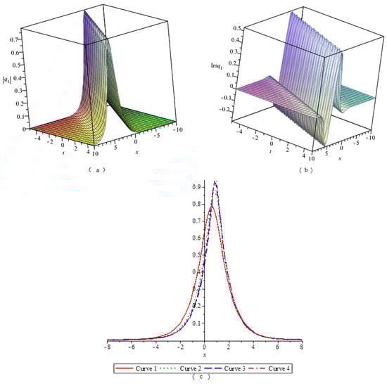
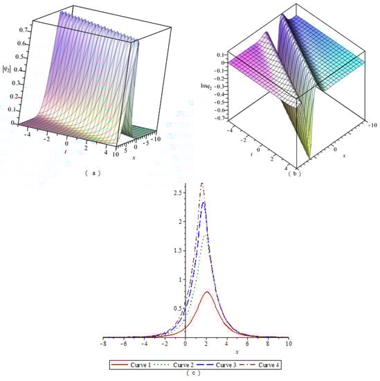
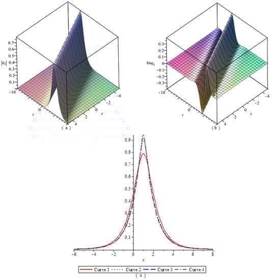
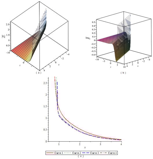
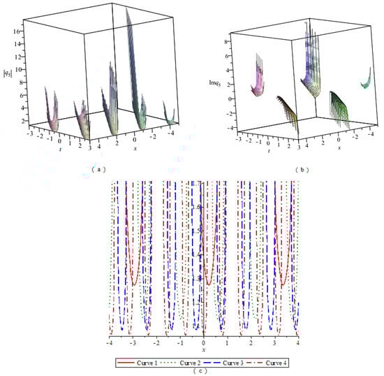
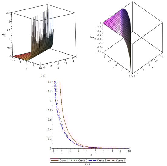
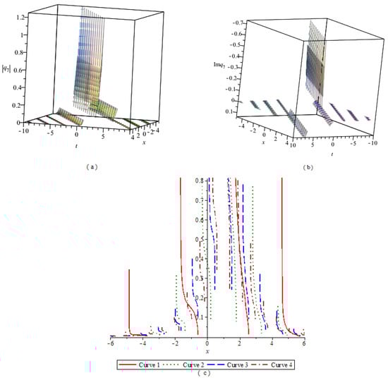
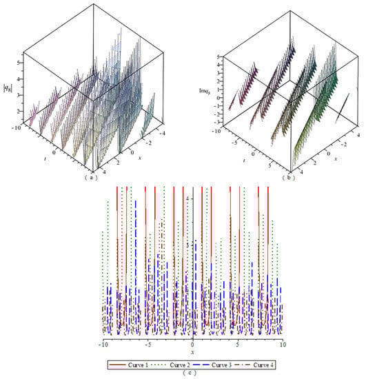
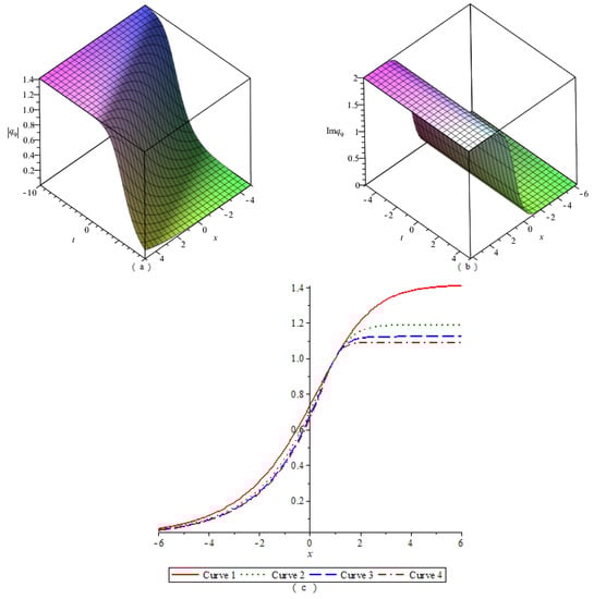
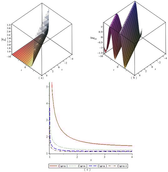
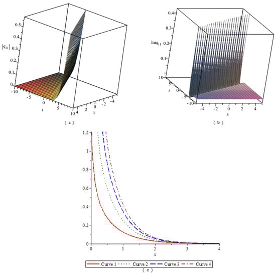
From Figure 1, Figure 2 and Figure 3, we observe that the module ($\left|q\right|$), which is a wave packet, is a solitary wave; the imaginary part is similar to a W-shaped solitary wave; the amplitude of the wave packet increases with the increase of $n=4$. Figure 4, Figure 6 and Figure 10 represent the wave structures of the singular soliton solution of Equation (2). Figure 5 and Figure 7 represent the wave structures of the periodic soliton solution of Equation (2). Figure 8 represents the wave structures of the singular-periodic soliton solution of Equation (2). Figure 9 represents the wave structures of the kink soliton solution of Equation (2). Figure 11 represents the wave structures of the exponential-type soliton solution of Equation (2).

5. Conclusions

In this paper, the new generalized Radhakrishnan–Kundu–Lakshmanan equations were transformed into the nonlinear ordinary differential equation using the complex envelope traveling wave solution. Some new solutions were obtained with the help of an auxiliary ordinary differential equation, and the wave structure was analyzed by graphical representations of the solution. The obtained solutions have not been reported in the existing literature. Clearly, the auxiliary ordinary differential equation is effective in obtaining exact solutions for some nonlinear partial differential equations.

References

- González-Gaxiola, O.; Biswas, A. Optical solitons with Radhakrishnan–Kundu–Lakshmanan equation by Laplace-Adomian decomposition method. Optik 2019, 179, 434–442. [Google Scholar] [CrossRef]
- Ghanbari, B.; Gómez-Aguilar, J.F. Optical soliton solutions for the nonlinear Radhakrishnan–Kundu–Lakshmanan equation. Mod. Phys. Lett. B 2019, 33, 1950402. [Google Scholar] [CrossRef]
- Ozisik, M.; Secer, A.; Bayram, M.; Yusuf, A.; Sulaiman, T.A. On the analytical optical soliton solutions of perturbed Radhakrishnan–Kundu–Lakshmanan model with Kerr law nonlinearity. Opt. Quant. Electron. 2022, 54, 371. [Google Scholar] [CrossRef]
- Ganji, D.D.; Asgari, A.; Ganji, Z.Z. Exp-Function Based Solution of Nonlinear Radhakrishnan, Kundu and Laskshmanan (RKL) Equation. Acta Appl. Math. 2018, 104, 201–209. [Google Scholar] [CrossRef]
- Biswas, A.; Yildirim, Y.; Yasar, E.; Mahmood, M.F.; Alshomrani, A.S.; Zhou, Q.; Moshokoa, S.P.; Belic, M. Optical soliton perturbation for Radhakrishnan–Kundu–Lakshmanan equation with a couple of integration schemes. Optik 2018, 163, 126–136. [Google Scholar] [CrossRef]
- Biswas, A. 1-Soliton solution of the generalized Radhakrishnan, Kundu, Lakshmanan equation. Phys. Lett. A 2009, 373, 2546–2548. [Google Scholar] [CrossRef]
- Arshed, S.; Biswas, A.; Guggilla, P.; Alshomrani, A.S. Optical solitons for Radhakrishnan–Kundu–Lakshmanan equation with full nonlinearity. Phys. Lett. A 2020, 384, 126191. [Google Scholar] [CrossRef]
- Tarla, S.; Ali, K.K.; Yilmazer, R.; Osman, M.S. The dynamic behaviors of the Radhakrish-nan-Kundu-Lakshmanan equation by Jacobi elliptic function expansion technique. Opt. Quant. Electron. 2022, 54, 292. [Google Scholar] [CrossRef]
- Lu, D.; Seadawy, A.R.; Khater, M.M.A. Dispersive optical soliton solutions of the generalized Radha-krishnan-Kundu-Lakshmanan dynamical equation with power law nonlinearity and its applications. Optik 2018, 164, 54–64. [Google Scholar] [CrossRef]
- Kudryashov, N.A. Solitary waves of the generalized Radhakrishnan–Kundu–Lakshmanan equation with four powers of nonlinearity. Phys. Lett. A 2022, 448, 128327. [Google Scholar] [CrossRef]
- Kudryashov, N.A. The Radhakrishnan–Kundu–Lakshmanan equation with arbitrary refractive index and its exact solutions. Optik 2021, 238, 166738. [Google Scholar] [CrossRef]
- Kudryashov, N.A.; Safonova, D.V.; Biswas, A. Painleve analysis and a solution to the traveling wave reduction of the Radhakrishnan–Kundu–Lakshmanan equation. Regul. Chaotic Dyn. 2019, 24, 607–614. [Google Scholar] [CrossRef]
- Alshehri, A.M.; Alshehri, H.M.; Alshreef, A.N.; Kara, A.H.; Biswas, A.; Yıldırım, Y. Conservation laws for dispersive optical solitons with Radhakrishnan–Kundu–Lakshmanan model having quadrupled power-law of self-phase modulation. Optik 2022, 267, 169715. [Google Scholar] [CrossRef]
- Annamalai, M.; Veerakumar, N.; Narasimhan, S.L.; Selvaraj, A.; Zhou, Q.; Biswas, A.; Ekici, M.; Alshehri, H.M.; Belić, M.R. Algorithm for dark solitons with Radhakrishnan–Kundu–Lakshmanan model in an optical fiber. Results Phys. 2021, 30, 104806. [Google Scholar] [CrossRef]
- Yildirim, Y.; Biswas, A.; Zhou, Q.; Alzahrani, A.K.; Belic, M.R. Optical solitons in birefringent fibers with Radhakrishnan–Kundu–Lakshmanan equation by a couple of strate gically sound integration architectures. Chin. J. Phys. 2020, 65, 341–354. [Google Scholar] [CrossRef]
- Seadawy, A.R.; Bilal, M.; Younis, M.; Rizvi, S.T.R.; Makhlouf, M.M.; Althobaiti, S. Optical solitons to birefringent fibers for coupled Radhakrishnan–Kundu–Lakshmanan model without four-wave mixing. Opt. Quant. Electron. 2021, 53, 324. [Google Scholar] [CrossRef]
- Wang, K.J.; Si, J. Optical solitons to the Radhakrishnan–Kundu–Lakshmanan equation by two effective approaches. Eur. Phys. J. Plus 2022, 137, 1016. [Google Scholar] [CrossRef]
- Yildirim, Y.; Biswas, A.; Ekici, M.; Triki, H.; Gonzalez-Gaxiola, O.; Alzahrani, A.K.; Belic, M.R. Optical solitons in birefringent fibers for Radhakrishnan–Kundu–Lakshmanan with five prolific integration norms. Optik 2020, 208, 164550. [Google Scholar] [CrossRef]
- Zhang, K.; He, X.; Li, Z. Bifurcation analysis and classification of all single traveling wave solution in fiber Bragg gratings with Radhakrishnan–Kundu–Lakshmanan equation. AIMS Math. 2022, 7, 16733–16740. [Google Scholar] [CrossRef]
- Miura, M.R. Bäcklund Transformation; Springer: Berlin/Heidelberg, Germany, 1978. [Google Scholar]
- Al Qurashi, M.M.; Baleanu, D.; Inc, M. Optical solitons of transmission equation of ultra-short optical pulse in parabolic law media with the aid of Backlund transformation. Optik 2017, 140, 114–122. [Google Scholar] [CrossRef]
- Wang, P.; Tian, B.; Sun, K.; Qi, F.-H. Bright and dark soliton solutions and Bäcklund transformation for the Eckhaus-Kundu equation with the cubic-quintic nonlinearity. Appl. Math. Comput. 2015, 251, 233–242. [Google Scholar] [CrossRef]
- Inc, M.; Aliyu, A.I.; Yusuf, A. Optical solitons to the nonlinear Shrödinger’s equation with spatio-temporal dispersion using complex amplitude ansatz. J. Mod. Opt. 2017, 64, 2273–2280. [Google Scholar] [CrossRef]
- Zhou, Q.; Zhu, Q.P. Optical solitons in medium with parabolic law nonlinearity and higher order dispersion. Waves Random Complex Media 2015, 25, 52–59. [Google Scholar] [CrossRef]
- Bekir, A.; Aksoy, E.; Güner, Ö. Optical soliton solutions of the long-short-wave interaction system. J. Nonlinear Opt. Phys. 2013, 22, 1350015. [Google Scholar] [CrossRef]
- Zayed, E.M.E.; Alngar, M.E.M.; El-Horbaty, M.; Biswas, A.; Alshomrani, A.S.; Khan, S.; Ekici, M.; Triki, H. Optical solitons in fiber Bragg gratings having Kerr law of refractive index with extended Kudryashov’s method and new extended auxiliary equation approach. Chin. J. Phys. 2020, 66, 187–205. [Google Scholar] [CrossRef]
- Kilic, B.; Inc, M. Soliton solutions for the Kundu-Eckhaus equation with the aid of unified algebraic and auxiliary equation expansion methods. J. Electromagnet. Wave 2016, 30, 871–879. [Google Scholar] [CrossRef]
- Zayed, E.M.E.; Alurrfi, K.A.E. Extended auxiliary equation method and its applications for finding the exact solutions for a class of nonlinear Schrödinger-type equations. Appl. Math. Comput. 2016, 289, 111–131. [Google Scholar] [CrossRef]
- Kader, A.H.A.; Latif, A.; Zhou, Q. Exact optical solitons in metamaterials with anti-cubic law of nonline-arity by Lie group method. Opt. Quant. Electron. 2019, 51, 30. [Google Scholar] [CrossRef]
- Iskenderoglu, G.; Kaya, D. Chirped self-similar pulses and envelope solutions for a nonlinear Schrödinger’s in optical fibers using Lie group method. Chaos Soliton Fract. 2022, 162, 112453. [Google Scholar] [CrossRef]
- Jafari, H.; Lia, A.; Tejadodi, H.; Baleanu, D. Analysis of Riccati differential equations within a new fractional derivative without singular kernel. Fundam. Inform. 2017, 151, 161–171. [Google Scholar] [CrossRef]
- Tajadodi, H.; Khan, Z.A.; ur Rehman Irshad, A.; Gömez-Aguilar, J.F.; Khan, A.; Khan, H. Exact solutions of conformable fractional differential equations. Results Phys. 2021, 22, 103916. [Google Scholar] [CrossRef]
- Yomba, E. The sub-ODE method for finding exact travelling wave solutions of generalized nonlinear Camassa-Holm, and generalized nonlinear Schrödinger equations. Phys. Lett. A 2008, 372, 215–222. [Google Scholar] [CrossRef]
Publisher’s Note: MDPI stays neutral with regard to jurisdictional claims in published maps and institutional affiliations. |
© 2022 by the authors. Licensee MDPI, Basel, Switzerland. This article is an open access article distributed under the terms and conditions of the Creative Commons Attribution (CC BY) license (https://creativecommons.org/licenses/by/4.0/).