Abstract
A new method aimed at endoscopic color images’ local contrast enhancement is proposed, based on local sliding histogram equalization with adaptive threshold limitation, color distortions correction, and image brightness preservation. For this, the original RGB image, represented as a tensor of size M × N × 3, is transformed into a matrix of size M × N, composed by the color vectors’ modules. As a result of local contrast enhancement, the obtained color vectors are symmetrical in respect of the input ones, because they satisfy the requirement for invariance after rotation. To enhance the local contrast, recursive local histogram equalization with adaptive thresholding is applied to each matrix element. This threshold divides the histogram into two regions of equal areas. A new metric for local contrast enhancement evaluation based on the mean square difference entropy is proposed. The presented new method is characterized by low computational complexity, due to the lack of direct and inverse color conversion and the possibility for adaptive local contrast enhancement, which is essential for accurate medical diagnosis based on endoscopic images analysis. In addition, the presented method performs both the correction of color distortions and the brightness preservation of each pixel.
1. Introduction
Improving the quality of endoscopic images obtained by specialized endoscopic equipment is essential for the correct medical diagnosis of the examined patient. A number of publications are known in which various approaches have been proposed to improve the quality of medical color images, and in particular—the endoscopic [1,2,3,4]. In [1], several systems for optical improvement of the endoscopic images’ quality are introduced, such as: the flexible spectral imaging color enhancement (FICE) system, image-enhanced endoscopy (IEE), and the auto fluorescence imaging (AFI) video endoscopic system. Linked color imaging (LCI) [2] is an endoscopic technique for color contrast enhancement, based on the RGB color model. For better lesions observation, white light imaging (WLI), LCI, and blue laser imaging (BLI) are used, i.e., various optical methods are developed to improve the image quality. In [3], a combination of WLI, LCI, and BLI techniques was used to diagnose gastric cancer. Patent US 10,516,962 B2 [4] relates to improving the quality of endoscopic images in the YCrCb color space, where the correlation between the luminance component Y and the two chromatic components Cr and Cb is significantly reduced. For this, the YCrCb model is converted into the nonlinear Lab model, whereby in order to reduce the noise due to values rounding, the number of bits per pixel for the component L is increased from 10 to 12 bits, and for each component a and b—from 8 to 10 bits, respectively. To increase the contrast, the CLAHE algorithm is used, which is applied to each L, a, b component. After this processing, the Lab model is converted into XYZ, and gamma correction is applied to each component obtained. In order to visualize the improved gamma endoscopic images on the screen, the corrected XYZ model is converted into RGB. The algorithm described in the patent is implemented using an FPGA. The main disadvantage of this approach is the high computational complexity due to the double nonlinear conversion of the used color models.
To improve the contrast of the processed endoscopic images, in [5], an YCrCb model is applied. After the direct transformation (RGB-YCrCb), the Y component only is processed and inverse conversion from YCrCb to RGB is performed. Here, Y is the luminance component and Cr and Cb are the chrominance components. The Y component is normalized and an adaptive sigmoid function is applied to it to improve the quality of the corresponding Y (brightness) image. The direct and inverse transforms of the YCrCb to RGB color model are linear, and in addition, provide a very good separation of the image brightness from the color. A disadvantage of the YCrCb model is the relatively high computational complexity to implement the transformation to RGB, which requires nine multiplications by fractions. This, in turn, results in errors due to rounding the pixel value of the restored image. One more disadvantage is that the output image with increased contrast does not retain the original predominant color.
An adaptive gamma correction (AGC) method has been proposed in [6] to improve the contrast of color RGB images. The AGC parameters are set dynamically by using the content information of each image. HSV color space is used, in which the information about the image color and brightness is divided into the following three components: for the color—the color tone (H) and the saturation (S), and for the brightness—the luminance (V). The selected HSV color model has a number of advantages, such as the ability to separate the color information from that of the brightness (lightness). For this reason, the improvement of the V-component does not change the original color of the pixels. The main disadvantages of the HSV model are the high computational complexity associated with the nonlinear nature of the transition from HSV to RGB (forward and inverse transforms), and the effect of error accumulation due to calculated values’ rounding. The approach introduced in [7] is similar to that from [6], and the HSV model is used again. The difference is in the image enhancement algorithm, which refers to the V component. The algorithm is based on Gaussian noise filtering and contrast enhancement of dark images by applying a locally transformed histogram-based technique. In [8] the HSI (Hue, Saturation, and Intensity) model is used instead of HSV. This color space also has the ability to separate the color information from that of hue and saturation. The model is suitable for processing images that represent lighting changes which is due to the fact that the colors of the environment are distinguishable from each other through the hue component. The RGB-HSI transformation is nonlinear and has higher computational complexity than RGB-HSV. The disadvantages of the HSI model are similar to these of HSV. To improve the quality of the color medical images, in this case, a selective chromatic filter is used to amplify one of the RGB components in the HSI space.
A new enhancement method which combines the Young–Helmholtz (Y-H) color transformation with adaptive equalization of the intensity matrix histogram is proposed in [9]. The adaptive histogram equalization (AHE) method is used to enhance the contrast and suppress the noise in the original image effectively. The enhanced image can be displayed in the RGB color space through inverse Y-H transformation with retained hue and saturation. The image enhancement is based on adaptive equalization of the intensity matrix histogram and the Y-H transformation, which have relatively high computational complexity. In [10], a method is proposed to improve the contrast of color images by histogram equalization of the modules of their color vectors. This method has not been studied for medical images (and in particular for endoscopic images), as it does not for their details (texture) to be visualized well enough.
The pixel components of the 24 bpp color images determine the coordinates of the color vectors whose vertices must be placed within a cube of size 256 × 256 × 256. As a result of the contrast enhancement, gamma correction, arithmetic operations between images, color, and geometric transformations, interpolation, etc., some of the components of the processed image may exceed the maximum allowable value of 255. If the maximum value of one of the components per pixel (i,j) is greater than 255, it should be reduced to 255 in order to be visually reproducible. In turn, this reduction changes the ratios between the values of the three components representing the color of the corresponding pixel, as a result of which its color changes. In general, the limitation of the maximum values of the image color components up to 255 results in color and luminance distortions.
The problem for color distortion correction of images obtained as a result of their brightness preserving has been the subject of a number of studies [11,12,13,14,15,16]. Histogram equalization (HE) is one of the common methods used to improve the contrast in digital images. However, this technique is not very well suited to be implemented in the medical decision support, because the method tends to introduce unnecessary visual deterioration, such as the saturation effect. One of the solutions to overcome this weakness is to preserve the mean brightness of the input (original) image in the output (result) image. In [11], a new method is proposed known as brightness preserving dynamic histogram equalization (BPDHE) that produces an output image whose mean intensity is almost equal to the mean intensity of the input, thus satisfying the requirement to retain the mean brightness of the image. In [12], a modification of the BPDHE technique is proposed to improve the brightness preserving and contrast enhancement abilities while reducing the computational complexity. The modified technique, called the brightness preserving dynamic fuzzy histogram equalization, uses the fuzzy statistics of the digital images for their representation and processing. An effective method for image contrast enhancement is presented in [13] based on a mapping function, which is a mixture of global and local transformation functions that improve both the brightness and the fine details of the original image. In [14], two image enhancement methods are introduced: weighted local and bidirectional smooth histogram stretching and local bidirectional smooth histogram stretching. A multiscale bilateral-weighted retinex method is proposed in [15] to remove the non-uniform and highly directional illumination and to enhance the surgical vision, while an objective no-reference image visibility assessment method is defined in terms of sharpness, naturalness, and contrast to quantitatively and objectively evaluate endoscopic visualization on surgical video sequences. In [16], before the histogram equalization, gamma and logarithmic transformation are executed on the input image in order to preserve the fine details. A new gamma value of the proposed algorithm helps to restrain the histogram spikes and to avoid over-enhancement and the noise artefacts effect. After that, a logarithmic transformation is used to map a narrow range of low-intensity values in the input image so as to ensure a wider range of the output levels. Thus, dark input values are spread out into the higher intensity values, which improves the overall image contrast and brightness.
In [17], a method is proposed to improve colors saturation during hue-preserving color image enhancement without the gamut problem. First, the color of each pixel in the input image is projected onto one of the three bisecting planes or bisectors of the RGB color cube to increase saturation. Then, that projected color is transformed into a target color with a designated luminance, retaining the original color hue. This method is characterized by unrealistically high color saturation and high computational complexity.
In order to avoid these disadvantages, a new method for correction of the color distortions of the processed images is proposed in our work, which also ensures their brightness preservation. The main objective is to develop and study a method and algorithm to improve the visual quality of the details in color endoscopic images by increasing their local contrast without color distortions and retaining the original brightness.
2. Main Features of the New Method for Local Contrast Enhancement
The main idea behind the new method for processing an RGB image represented as a tensor of size M × N × 3 is to transform it into an equivalent matrix of size M × N. In this way, three-dimensional color image processing can be replaced by simpler two-dimensional processing. For this purpose, the module of the corresponding color vector is calculated for each pixel of the RGB image. The result is an MxN matrix whose elements are the color vectors’ modules. The new local contrast enhancement algorithm for color RGB images (described below in detail) is based on the recursive sliding window for local contrast-limited histogram equalization (RSW-LCLAHE) with local brightness preservation.
The common feature of the new method RSW-LCLAHE is that there is no need to convert the RGB space into another color space, such as YCrCb, HSV, HSI, HLS, Lab, YUV, etc. [4,5,6,7,8]. Instead, a different approach is used: after increasing the contrast of the color vector C = [R,G,B]T, which represents the color of each pixel of the original image, only its module is changed, but its direction in the RGB space is preserved. This changes only the color saturation of each pixel retaining its color tone. The lack of conversion of RGB components into those for brightness and chromaticity used in the known contrast enhancement methods significantly reduces the computational complexity of the RSW-LCLAHE method proposed here, because it is performed through adaptive equalization of the local histogram, determined by the modules of all color RGB vectors in a square sliding window.
The algorithm RSW-LCLAHE is applied on the module of the color vector in the center of the sliding square window. As a result, the local contrast enhancement increase for each color pixel is an advantage of great importance for the medical diagnosis accuracy obtained through visual or computer-aided analysis of endoscopic images.
3. Main Steps of the Algorithm for the Proposed Method
The Algorithm Includes the following Main Steps
Step 1. Transformation of the tensor XC into a series of color vectors’ modules.
The transformation of the color tensor XC composed of matrices R, G, B each of size M × N with b bpp, into series of color vectors for i/j = 1, 2, …, M/N (vectorization of tensor XC), is presented in Figure 1. The so obtained vectors are symmetrical in respect to the input ones because they satisfy the requirement for rotation invariance (the direction of the input and the output vectors are the same). The vertices of the color vectors define the color space of the image.
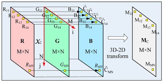
Figure 1.
Transformation of RGB tensor of size M × N × 3 into a M × N matrix of color vectors’ modules.
In Figure 2, the color space within the RGB cube in a sphere with radius MC = 442 for b = 8 bpp and the Maxwell’s triangle defining the reproducible colors on the screen are given.
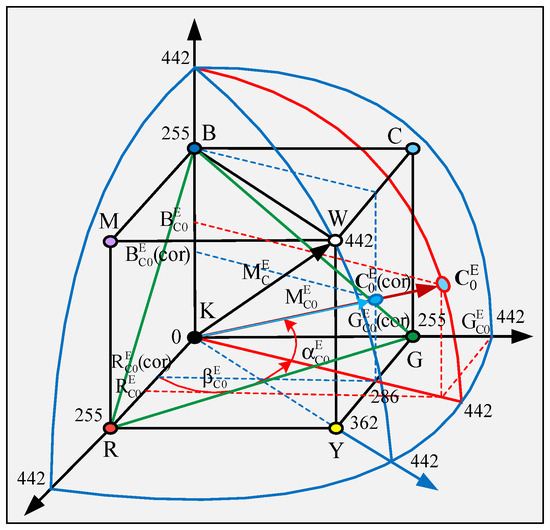
Figure 2.
RGB cube in a sphere with radius MC = 442. The color vector marked with red. is outside of the RGB cube. Its component must be reduced to 255. Maxwell’s triangle is given in green.
The relationship between the orthogonal and angular coordinate systems (R,G,B) and (MC, α, β), is:
Then
The elements of the matrix MC, composed of the modules of the color vectors , are defined by the expression:
Step 2. Sliding histogram equalization of color vectors’ modules.
Step 2.1. Definition of color vectors for p,q = 0, ±1, ±2, …, ±d, which compose the tensor XC,i,j, (3D sliding red window of size (2d + 1) × (2d + 1) × 3 for d = 1 in accordance with Figure 3); (p,q)—local coordinates in the 2D sliding window; (i,j)—global 2D coordinates of the pixel (i,j) for i/j = 1, 2, …, N/M within each matrix R, G, B.
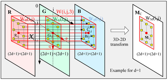
Figure 3.
Transformation of the 3D sliding window (tensor of size 3 × 3 × 3 for d = 1) into a 3 × 3 sliding matrix Mi,j.
Step 2.2. Transformation of the tensor XC,i,j (3D sliding window with a central element (i,j) within the matrix G) into a series of color vectors (vectorization of the tensor XC,i,j).
Step 2.3. Calculation the RGB vectors’ modules in the 2D sliding window WM(i,j) for i/j = 1, 2, …, N/M (within the matrix MC, in accordance with Figure 3):
for .
Step 2.4. Calculation of the normalized RGB vectors:
where for p, q = 0, ±1, ±2, …, ±d.
Step 2.5. Calculation of the local histogram for a sliding window WM(i,j) of the RGB vectors’ modules:
where nc,i,j(k) denotes the number of pixels, for which the module MC of the corresponding non-normalized vectors is at value k for p,q = 0, ±1, ±2, …, ±d, when the window WM(i,j) is of size (2d + 1) × (2d + 1).
Step 2.6. Equalization of the local contrast-limited adaptive histogram of color vectors’ modules based on the recursive sliding window.
To improve the contrast of the central pixel in the 2D recursive sliding window WM(i,j) only, it is necessary to calculate in advance the so-called truncation threshold surface (TTS), which covers all elements of the matrix MC of the color vectors’ modules. Each element MC(i,j) of this matrix is used to define a corresponding individual threshold CLi,j, through which the contrast-limited adaptive histogram equalization is performed. This accelerates the calculation of CLi,j, since it is not required for the local histogram for each element MC(i,j) within the sliding window WM(i,j) to be calculated.
Step 2.6.1.Calculation of the truncation threshold surface.
The matrix of the RGB vectors’ modules MC is of size M × N and with elements MC(i,j) for i = 1, 2, …, M, j = 1, 2, …, N. The matrix MC is divided into (MN)/Q2 non-overlapping blocks MC,u,v (each of size Q × Q elements), for Q = 2s + 1 and u = 1, 2, …, (M/Q) (number of blocks in horizontal direction) and v = 1, 2, …, N/Q (number of blocks in vertical direction). For each block MC,u,v is calculated for the corresponding individual threshold CLu,v. It is used to calculate the truncation thresholds surface—the matrix T of size M × N, which comprises blocks Tu,v ≡ MC,u,v. In the space, defined by the centers of each four spatially-neighboring blocks Tu,v, Tu+1,v, Tu,v+1, Tu+1,v+1, is defined the matrix Tu,v of size Q × Q with elements tu,v(α,β) for α,β = 0,1,..,Q-1. The following symbols are introduced for the corner elements of the matrix Tu,v, resp.: tu,v(0,0) = A, tu+1,v(Q,0) = B, tu,v+1(0,Q) = C, tu+1,v+1(Q,Q) = D. In this case, A, B, C, and D coincide with the thresholds CLu,v, CLu+1,v,CLu,v+1, CLu+1,v+1 for the group of four spatially-neighboring blocks Tu,v, Tu+1,v, Tu,v+1, Tu+1,v+1. The remaining elements tu,v(α,β) of the matrix Tu,v are calculated through BLI (bilinear interpolation) in correspondence with the relation:
Here, (α0,β0) are the local coordinates of the element tu,v(α0,β0) of the matrix Tu,v = [tu,v(α0,β0)].
Step2.6.2. Calculation of the adaptive threshold.
To define the adaptive threshold , here it is assumed that its value must depend on the distribution of the local histogram for the block Tu,v. In our approach, the threshold is calculated so as to divide the area of the local histogram into two equal in area parts, in accordance with Figure 4. The two parts of the histogram are defined in correspondence with the relations below:
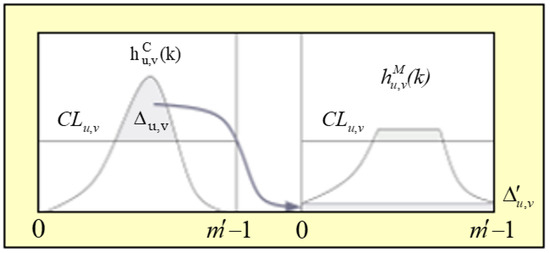
Figure 4.
Setting the value of the threshold CLu,v for the local histogram .
In this case . A notation is entered for the number of grey levels per element: ; is the height of a rectangle with dimensions and area , defined by the histogram portion above the threshold CLu,v, where .
The value of the threshold CLu,v is in the range 0 < CLu,v < 1. The choice of CLu,v in this range is based on the following considerations:
- -
- The reduction of CLu,v increases the area of the histogram above the threshold and, respectively, that of . As a result, the image brightness within the Tu,v block increases and the contrast decreases;
- -
- The increase of CLu,v reduces the area of the upper part of the histogram and respectively—of . As a result, in the dark region of the Tu,v (background), the contrast of the details in the image increases, but the contrast of the noise increases as well.
Therefore, the threshold value of is chosen as a compromise between the two alternatives mentioned above, following the condition for areas equality of the histograms and , i.e.,:
The symmetry of the two parts of the local histogram areas after its division by the threshold is one of the main differences between the RSW-LCLAHE introduced here and the well-known CLAHE. As a result of the application of RSW-LCLAHE with an adaptive threshold, the maximum contrast of the central element of the block Tu,v is provided due to the maximum linear stretching of its histogram without loss of grey levels, together with minimal noise contrast increase.
The threshold is calculated by using the following iterative algorithm of four steps. Let , with initial values x = 0, and δ = 0.01.
To define the threshold CLi,j for the histogram truncation in the window WM(i,j) for the module MC(i,j) in the global coordinate system (i,j) for i = 0,1,..,M−1 and j = 0,1, …, N−1, it is necessary to take into account the displacement (Δiu, Δjv) of the origin of the local coordinate system of the block, regarding the global coordinate system. Then, the needed local threshold CLu,v(I,j) for the module MC(i,j) from the block Tu,v, is defined by the relation:
for u = 1, 2, …, (M/Q); v = 1, 2, …, (N/Q); i = 0, 1, …, M − 1; j = 0, 1, …, N − 1;
The so-presented algorithm for CLu,v(i,j) definition must be executed before the RSW-LCLAHE algorithm. To simplify the explanations, in the description below, the indices u,v of the local threshold CL(i,j), and, respectively, of the element t(i,j) of the matrix T, will not be used because they are a function of variables (i,j) only.
Step2.6.3. Sliding window contrast-limited adaptive histogram equalization.
The algorithm for local contrast-limited adaptive histogram equalization is designed to enhance the contrast of each element of the input matrix based on the elements in the sliding window that it covers. The local histogram is calculated for the elements in the sliding window W(i,j) whose central element is MC(i,j):
Here is the number of pixels in the sliding window WM(i,j) of size (2b + 1) × (2d + 1), whose center coincides with the element MC(i,j);
—the number of elements MC(i + p,j + q) with grey level value k in the sliding window WM(i,j).
The calculation of the modified local histogram for the sliding window WM(i,j) in correspondence with the RSW-LCLAHE algorithm is performed in accordance with the the expression below:
where is the basic level to lift the modified local histogram . The calculation of the modified local cumulative histogram for the element (i,j) of matrix MC(i,j) is performed in accordance with the relation:
The calculation of the new grey level zk(i,j) of 12 bits per element (i,j) from the enhanced matrix, which replaces the grey level value k of the 10 bits per element MC(i,j) from the input matrix, and is used as the brightness value for the center of the sliding window WM(i,j), is:
As a result, the modified matrix with elements zk(i,j) is obtained, whose truncated histogram is equalized. Through increasing the number of bits per element of the matrix MC with improved contrast, the appearance of false contours in areas with the same levels of grey is avoided. In the description below, the grey level k of the element z(i,j) will not be used because it depends only on the variables (i,j).
Step3. Recursive calculation of the modified local histogram.
The recursive calculation of the modified local histogram within the sliding window WM(i,j) around each element MC(i,j) is only intended to speed up the contrast enhancement process by using the described sliding equalization algorithm. The sliding window WM(i,j) is moved one position ahead in a horizontal direction so that its center coincides with the element MC(i + 1,j). For the new position of the window, WM(i + 1,j) is recursively calculated for the corresponding local modified histogram .
where and are the modified histograms with grey level k in the first column (i-d) of the window WM(i,j) with center (i,j), and in the last column (i-d + 1) of the window (i + 1,j) with center (i + 1,j), respectively. Here CLi+1, j is the threshold value for the histogram of the elements in the window with center MC(i + 1,j). The modified histogram for the first column (i-d) of the window WM(i,j) is:
where for . ;
The modified histogram for the last column (i + d + 1) of the window WM(i + 1,j) is:
where for ;
For each next window position when i = d + 2, d + 3, …, M-d and j = d + 2, d + 3,..,N-d, the previous steps are executed again. The initial position of the window is defined by the element MC(d + 1, d + 1), and the window moves to the next position from left to right and to the next row below. Unlike the well-known CLAHE algorithm, the RSW-LCLAHE algorithm offered here is using a sliding window placed around each element, whose histogram has an individual clipping factor (CL) based on the truncation threshold surface (TTS).
The calculation of the local modified histogram is accelerated through recursion in accordance with Figure 5.
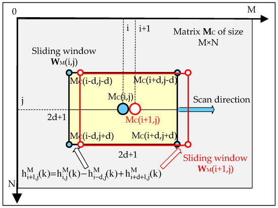
Figure 5.
Two consecutive positions of the sliding window: WM(i,j) and WM(i + 1,j).
The ratio η between the number of additions needed to compute the modified local histogram for the element (i,j) in a non-recursive manner in accordance with expression (18) and the recursively based on the same histogram for the preceding element (i−1,j) in accordance with expression (21) is defined by the relation:
From this equation it follows that as d increases in result of the recursion, the computation of accelerates. So, for a sliding window of size 3 × 3, η(1) = 2 while for a window of size 33 × 33, the acceleration reaches η(16) = 17 times.
Step 4. Calculation of the RGB vectors of the enhanced image.
where .
Step 5. Adaptive correction of the enhanced image color components placed outside the RGB cube, with brightness preservation:
First, it is checked whether the coordinates of the vector in the center of the sliding window fall outside the color RGB cube of size 256 × 256 × 256 in accordance with Figure 2. For example, the color vector marked with red is outside the RGB cube.
Then, the number NC of the color vectors C that are outside the RGB cube is detected. The condition is checked for correction of the modules of color vectors NC ≥ δ, where δ is a pre-selected threshold. If this condition is not met (NC < δ), then the color vector modules of all pixels in the image are corrected as follows:
Step 5.1. If for the red component of the vector for the pixel (i0,j0) satisfies the condition , the following correction is performed to avoid color vectors positioning outside the color cube:
Since according to Recommendation ITU-R BT.709 [18]: Y = 0.21R + 0.72G + 0.07B, then
The brightness of the original image pixel (i0,j0) according to Rec. ITU-R BT.709 is:
Therefore, the ratio shows how much the brightness is increased as a result of the processing and the following correction. Preserving the brightness of the output (enhanced) image regarding the input image permits improvement of the diagnostic results based on visual observation. As is known [19], the image brightness controls the human eye adaptation and accommodation regarding the observed objects in the image so as to improve their visual quality.
To preserve the image brightness, one more correction must be carried out:
For the remaining vectors , components correction is needed:
Then, brightness preservation must be carried out by using , as follows:
Step 5.2. If for the green component of the vector for the pixel (i0,j0) satisfies the condition , the following correction is performed to avoid the appearance of color vectors outside the color cube:
Brightness correction:
For the brightness preservation, a second correction must be carried out through , as follows:
For the remaining vectors , the corrected components are:
Then, brightness preservation must be carried out by using , as follows:
Step 5.3. If for the blue component of the vector for the pixel (i0, j0) satisfies the condition , the following correction is performed to avoid the appearance of color vectors outside the color cube:
The brightness correction for is performed as follows:
For the remaining vectors , after components correction is obtained:
Then, brightness preservation must be carried out by using , as follows:
Step 5.4. If for vectors of all pixels (i,j) for i/j = 1, 2, …, M/N satisfies the requirement , then
Step 6.Calculation of the output-enhanced and -corrected RGB vector, :
where for s = 1, 2, 3, 4.
Output: The enhanced color tensor of size M × N × 3, defined after folding of the output enhanced color vectors for i/j = 1, 2, …, M/N.
The pseudocode of the described Algorithm 1 follows below.
| Algorithm 1. Local contrast enhancement using sliding histogram equalization of color vectors’ modules |
| Input: of size , with 3b bits per voxel Output: The enhanced of with 3b bits per voxel for unfold() // Vectorization // of tensor lateral mode-3 (tube) complete Equations (5)–(7), normalization of // calculation for 2D sliding // window for complete Equation (8) // Calculation of blocks of the // truncation matrix T // Recursive sliding window for contrast-limited adaptive local histogram // equalization complete Equation (10)// Calculation of parts of local histogram, // complete Equations (11)–(14) // Calculation of threshold using iterative algorithm complete Equations (15) and (16) // Define local threshold for each module // using truncation matrix complete Equations (17)–(20) // Executing RSW-LCLAHE for contrast // enhancement complete Equations (21)–(23) // Executing recursive RSW-LCLAHE for contrast // enhancement complete Equation (25) // Calculation of the RGB vectors of enhanced image // Adaptive correction of color components // There are pixels in component of color vectors outside the RGB cube if complete Equation (26) else complete (30) // Correction for the remaining vectors // If there are pixels in component of color vectors outside the RGB cube if complete Equation (32) or else complete (35) // Correction for the remaining vectors // If there are pixels in component of color vectors outside the RGB cube If complete Equation (37) or else complete (39) // Correction for the remaining vectors // If for all pixels (i,j) i/j = 1, 2, …, M/N in color vectors there are not pixels outside the RGB cube If , complete Equation (41) // Calculation of the output enhanced and corrected RGB color vectors complete Equation (44) // Transform color vectors into tensor of size for // complete end |
4. Results for Local Contrast Enhancement of Endoscopic Images
Some results of the application of the developed algorithms for local contrast enhancement of endoscopic images are shown in Figure 6, Figure 7 and Figure 8. The choice of the sliding window size for the local contrast enhancement is important from the point of view of increasing the contrast of smaller or larger details or objects in the image, which are important for doctors in the diagnosis of disease based on visual evaluation of the endoscopic images of the patient. Therefore, the paper presents contrast enhancement results at different window sizes of 17, 33, and 65 to illustrate the difference in contrast enhancement of smaller or larger details or objects in the selected test images.
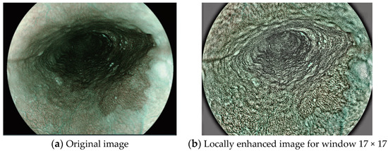
Figure 6.
Results for blue laser endoscopic image.
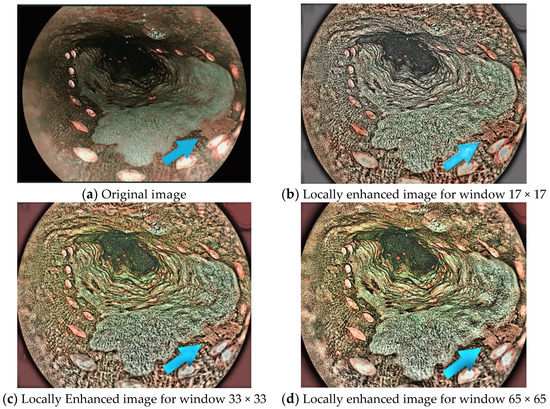
Figure 7.
Results for endoscopic image of squamous esophageal cells for different window sizes.
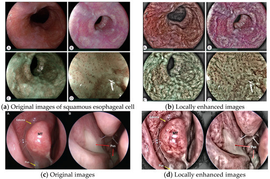
Figure 8.
Local contrast enhancement of different types of endoscopic color images for a window 17 × 17.
5. Metrics for Contrast Enhancement Evaluation
For the quantitative evaluation of the image quality enhancement, various criteria are developed [20] which correspond to different image classes, such as photos, video sequences (greyscale and color), underwater, multispectral, and medical (ultrasound, computer tomography sequences, medical photos, etc.). In general, many methods and algorithms exist for objective assessment of the image contrast enhancement degree. Potentially, all of these can be used in selecting an appropriate metric to evaluate the contrast enhancement. In this article, only metrics that are specific and widely used in the contrast enhancement assessment of medical imaging are presented below.
5.1. Contrast Per Pixel (CPP)
The value of the CPP is used to represent the local contrast in the image
where x(i,j) is the grey value and x(i + m, j + n) is the neighbor pixel x(i,j) in a 3 × 3 window.
5.2. Absolute Mean Lightness Difference (AMLD)
Absolute mean grey lightness difference is defined as the absolute difference between the mean grey value of the original image and that of the lightened/darkened image:
where and are the mean grey level values of the input and output image, respectively.
5.3. Mean Square Difference Entropy (MSDE)
The value of MSDE is calculated by the following formula
where denotes the local entropy (LE) in the sliding window; x1(i,j) and x0(i,j) are the grey level values of the pixels in the output and the input image, respectively; m—the number of grey levels in the image.
After conducting tests with each of the presented metrics for evaluating local contrast enhancement, the metric represented by Expression (47) was adopted and used.
6. Analysis of Local Contrast Enhancement Results for Color Endoscopic Images with the Proposed Sliding Histogram Equalization
The experiments for local contrast enhancement with the proposed sliding histogram equalization were carried out with the chosen samples from the existing suitable database of 76 color endoscopic images [21] of type “Hyperplasic Lesions”. We have conducted experiments on a large number of these images, but for brevity, the paper presents results of applying the proposed algorithm for local contrast enhancement to image 1 only (hyperplasic_01 from the database). In addition, apart from numerous experiments with images from the abovementioned database of endoscopic images, the paper conducts for comparison experiments with other, other than those in the image database, types of medical images used in some of the articles cited in the introduction. From the experiments with these other types of medical images, the results are presented for brevity only for images 2 and 3 (serrated lesions and adenoma), respectively. In order to conduct the tests, corresponding software programs were developed based on the proposed algorithm for local contrast enhancement (LCE) of color endoscopic images. In addition, the appropriate programs were prepared for assessing the degree of the achieved local contrast enhancement using the proposed sliding histogram equalization of color endoscopic images.
The results from the tests carried out for the local contrast enhancement of color endoscopic images, using the developed corresponding programs, are shown in Table 1. The tests were performed with a lot of color endoscopic images from the database, but in Table 1, only three test images are shown, named in the first column as Image 1, Image 2, and Image 3. The choice of these images is made to present the results from the more important types of color endoscopic images: hyperplasic and serrated lesions and adenoma. In the second column of Table 1, the input color endoscopic images chosen from the database of color endoscopic images are shown [21]. The next three columns are for output color endoscopic Image 1, Image 2, and Image 3 after local contrast enhancement, after maximal values of RGB components correction to 255, and after brightness correction, respectively.

Table 1.
Images from the test database used for local contrast enhancement (LCE).
The results for the local contrast enhancement are shown for three typical cases of sliding windows size: 17 × 17; 33 × 33 and 65 × 65, to show the difference, depending on the sliding windows’ size.
The summarized results for the achieved contrast enhancement degree using the proposed local sliding histogram equalization of color endoscopic images are given in Table 2. The experiments were carried out with the program implementing the method presented in Section 5.3 for the mean square difference entropy (MSDE) calculation.
Table 2.
MSDE estimation of the achieved local contrast enhancement (LCE).
This method ensures better correspondence between the objective assessment (using the contrast enhancement estimation) and the subjective perception of the contrast enhancement.
The following abbreviations are used in Table 2: I/E—the MSDE between the input and output image with enhanced contrast; I/C—the MSDE between the input and output image with enhanced contrast and maximal values (255) for the RGB components; I/C/I—the MSDE between the input and output image with enhanced contrast, with corrected maximal values for the RGB components and intensity correction. The endoscopic images 1, 2, and 3 were also used for contrast enhancement tests with the well-known CLAHE algorithm [22]. The results for the visual comparison and the MSDE estimation of the achieved contrast enhancement using RSW-LCLAHE and CLAHE are shown in Table 3.
Table 3.
Results for RSW-LCLAHE and CLAHE.
Analyzing the results from Table 2, after estimation of the contrast enhancement degree achieved using the proposed local sliding histogram equalization for contrast enhancement of color endoscopic images, the following conclusions can be made:
- -
- The degree achieved using the local sliding histogram equalization for contrast enhancement depends on the choice of the sliding window size and is higher for smaller windows (example case 17 × 17 from Table 2) when compared to a larger sliding window (example case 65 × 65 from Table 2), but the textural structure is more noticeable for smaller windows (example case 17 × 17 from Table 1) when compared to a larger sliding window (example case 65 × 65 from Table 1);
- -
- The contrast enhancement, achieved using the local sliding histogram equalization depends on the choice of the sliding window size and is higher for smaller windows (for the example case 17 × 17 from Table 2) compared to the larger sliding window (for the example case 65 × 65 from Table 2), but the textural structure is more noticeable for smaller windows (for the example case 17 × 17 from Table 1) when compared to a sliding window of a larger size (for the example case 65 × 65 from Table 1). The size of the sliding square window is chosen so that the window covers the objects whose local contrast needs enhancement;
- -
- The analysis of the results from Table 2 and Table 3, for the estimation of MSDE contrast enhancement for endoscopic images 1, 2, and 3, shows significantly higher MSDE values, when the proposed local sliding histogram equalization is used, compared to the MSDE values obtained using the well-known CLAHE algorithm [22];
- -
- From the quantitative results for MSDE, given in Table 2 and from the visual perception of the enhancement endoscopic images 1, 2, and 3, shown enlarged in Figure 9, it can be concluded that for each medical application, it is preferable to choose the size of sliding window for histogram equalization so as to achieve the corresponding local contrast enhancement in the desired Region Of Interest (ROI); for example, a smaller sliding window for a smaller ROI, or larger one in case of a larger ROI.
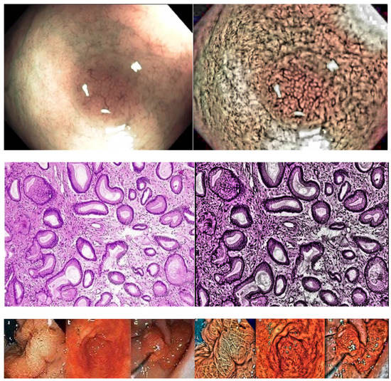 Figure 9. The enlarged input (on the left) and output (on the right) contrast-enhanced endoscopic images 1, 2, and 3 after using the proposed method for local sliding histogram equalization.
To obtain better visual perception of the achieved contrast enhancement quality using the proposed local sliding histogram equalization, the enlarged input (on the left) and output (on the right) contrast enhanced endoscopic images 1, 2, and 3 are shown in Figure 9.
The comparison results for the MSDE values obtained through RSW-LCLAHE and CLAHE algorithms for Image 1 in accordance with row one from Table 2 and row one from Table 3, are shown in graphic form as an example in Figure 10.
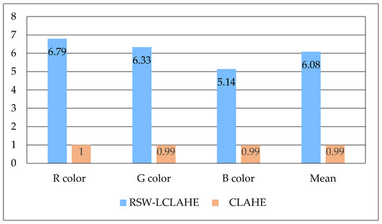
Figure 10.
Comparison of MSDE results for Image 1 obtained through RSW-LCLAHE and CLAHE.
The results of testing a big number of test endoscopic images obtained by applying CPP and AMLD to evaluate the contrast enhancement showed insignificant values between 0.3–1.1 for both RSW-LCLAHE and CLAHE. This can be explained by the fact that according to Equation (45), CPP is calculated by local averaging of the pixels in a sliding window of a minimum size 3 × 3, while according to equation (46), AMLD is calculated by global averaging of the entire image. Subjective evaluation, however, shows a significant increase in contrast. This evaluation is prioritized for the visual analysis of the processed endoscopic images, which is a good prerequisite for improving diagnosis accuracy. Compared to CPP and AMLD, the MSDE criterion defined by equation (47) is the most suitable for objective evaluation of contrast enhancement by applying RSW-LCLAHE and CLAHE. This choice is due to the very good coincidence of the results of the objective evaluation, for which the values for the increased contrast reach 6.79 (see Table 2) with those of the subjective evaluation.
7. Conclusions
The main scientific results of our work, which distinguish it from other similar works, are as follows:
- -
- A new method is developed for contrast enhancement of color endoscopic image, represented as RGB tensor of size M × N × 3, transformed into the M × N matrix of the color vectors’ modules. The three-times smaller volume of data achieved in this matrix, compared to that of the tensor, results in lower computational complexity of the corresponding algorithm. The transformation of the RGB tensor XC into the corresponding matrix MC requires 6MN arithmetic operations, while the linear straight and inverse RGB-YCrCb transformation requires 30MN arithmetic operations, i.e., five times more. For nonlinear conversions such as RGB-HSV, RGB-HSI, RGB-YHT, etc., the number of operations increases significantly compared to that for the linear ones. The comparison of the overall computational complexity of the proposed method with that of the global contrast enhancement methods is not correct, because RSW-LCLAHE enhances the local contrast of each element of the MC matrix based on the histogram of the surrounding elements in a window of size (2d + 1) × (2d + 1). The increase of the parameter d leads to a linear acceleration of the proposed algorithm for recursive calculation of the histogram compared to the non-recursive one;
- -
- Development and research of a method aimed at the visual quality improvement of color endoscopic images through increasing their local contrast without color distortion and retaining their mean brightness compared to the original images;
- -
- A new method for correction of color distortions of the processed images is developed, which at the same time preserves the mean brightness of processed images;
- -
- A new algorithm is developed for calculation of the adaptive threshold which limits the local histogram of the color vectors’ modules by dividing it into two equal-area parts;
- -
- A new metric for local contrast enhancement evaluation based on MSDE is proposed, providing a good match with the subjective image evaluation.
The results obtained from the research of the developed algorithms for processing color endoscopic images show very good opportunities for their application as a tool to support medical practices related to accurate diagnosis. We believe that the developed method can be successfully applied to other types of medical images that we have not investigated at this stage.
The future development of the new color tensor image processing approach could be summed up for transformation and analysis of sequences of correlated color tensor images. Considering the results in [23], it can be expected that the use of the RSW-LCLAHE algorithm for preprocessing of endoscopic images will increase the accuracy of neural networks designed to detect various diseases in the early phase of their development.
Author Contributions
Conceptualization, R.K., A.B., R.M. and S.P.; methodology and formal analysis, R.M.; investigation, A.B.; writing—original draft preparation, R.K.; writing—review and editing, S.P.; visualization, R.K. All authors have read and agreed to the published version of the manuscript.
Funding
This work was funded by the Bulgarian National Science Fund: Project No. KP-06-H27/16: “Development of efficient methods and algorithms for tensor-based processing and analysis of multidimensional images with application in interdisciplinary areas”.
Institutional Review Board Statement
This study does not require ethical approval.
Informed Consent Statement
Not applicable.
Data Availability Statement
Not applicable.
Conflicts of Interest
The authors declare no conflict of interest. The funders had no role in the design of the study; in the collection, analyses, or interpretation of data; in the writing of the manuscript; or in the decision to publish the results.
References
- Yoshida, N.; Yagi, N.; Yanagisawa, A.; Naito, Y. Image-enhanced endoscopy for diagnosis of colorectal tumors in view of endoscopic treatment. World J. Gastrointest. Endosc. 2012, 4, 545–555. [Google Scholar] [CrossRef] [PubMed]
- Sun, X.; Dong, T.; Bi, Y.; Min, M.; Shen, W.; Xu, Y.; Liu, Y. Linked Color Imaging Application for Improving the Endoscopic Diagnosis Accuracy: A Pilot Study. Sci. Rep. 2016, 6, 33473. Available online: www.nature.com/scientificreports (accessed on 2 December 2022). [CrossRef] [PubMed]
- Osawa, H.; Miura, Y.; Takezawa, T.; Ino, Y.; Khurelbaatar, T.; Sagara, Y.; Lefor, A.; Yamamoto, H. Linked Color Imaging and Blue Laser Imaging for Upper Gastrointestinal Screening, Korean Society of Gastrointestinal Endoscopy. Clin. Endosc. 2018, 61, 513–526. [Google Scholar] [CrossRef] [PubMed]
- Sidar, I.; Davidson, T.; Kronman, A.; Mor, L.; Levy, E. Endoscopic Image Enhancement using CLAHE Implemented in a Processor. Patent No. US 10,516,865 B2, 24 December 2019. [Google Scholar]
- Imtiaz, M.; Wahid, K. Color Enhancement in Endoscopic Images Using Adaptive Sigmoid Function and Space Variant Color Reproduction. Comput. Math. Methods Med. 2015, 2015, 607407. [Google Scholar] [CrossRef] [PubMed]
- Rahman, S.; Rahman, M.; Abdullah-Al-Wadud, M.; Al-Quaderi, G.; Shoyaib, M. An adaptive gamma correction for image enhancement. EURASIP J. Image Video Processing 2016, 2016, 35. [Google Scholar] [CrossRef]
- Hussain, K.; Rahman, S.; Rahman, M.; Khaled, S.; Wadud, M.A.; Khan, M.; Shoyaib, M. A histogram specification technique for dark image enhancement using a local transformation method. Trans. Comput. Vis. Appl. 2018, 10, 1–11. [Google Scholar] [CrossRef]
- Blotta, E.; Bouchet, A.; Ballarin, V.; Pastore, J. Enhancement of medical images in HSI color space, XVIII Congreso Argentino de Bioingeniería SABI 2011—VII Jornadas de Ingeniería Clínica, Mar del Plata, 28 al 30 de septiembre de 2011. J. Phys. Conf. Ser. 2011, 332, 012041. [Google Scholar] [CrossRef]
- Gu, J.; Hua, L.; Wu, X.; Yang, H.; Zhou, Z. Color Medical Image Enhancement Based on Adaptive Equalization of Intensity Numbers Matrix Histogram. Intern. J. Autom. Comput. 2015, 12, 551–558. [Google Scholar] [CrossRef][Green Version]
- Lamont, F.; Cervantes, J.; Chau, A.; Ruiz, S. Contrast Enhancement of RGB Color Images by Histogram Equalization of Color Vectors’ Intensities; Huang, D., Ed.; LNAI 10956; Springer Intern. Publishing ICIC: Wuhan, China, 2018; pp. 443–455. [Google Scholar] [CrossRef]
- Ibrahim, H.; Kong, N. Brightness Preserving Dynamic Histogram Equalization for Contrast Enhancement. Electron. IEEE Trans. Consum. 2007, 53, 1752–1758. [Google Scholar] [CrossRef]
- Sheet, D.; Garud, H.; Suveer, A.; Mahadevappa, M.; Chatterjee, J. Brightness Preserving Dynamic Fuzzy Histogram Equalization. IEEE Trans. Consum. Electron. 2010, 56, 2475–2480. Available online: https://www.researchgate.net/publication/224209829 (accessed on 2 December 2022). [CrossRef]
- Kabir, H.; Wadud, A.; Chae, O. Brightness Preserving Image Contrast Enhancement Using Weighted Mixture of Global and Local Transformation Functions. Int. Arab. J. Inf. Technol. 2010, 7, 403–410. [Google Scholar]
- Kotkar, V.; Gharde, S. Image Contrast Enhancement by Preserving Brightness Using Global and Local Features. In Proceedings of the Third International Conference on Computational Intelligence and Information Technology (CIIT 2013), Mumbai, India, 18–19 October 2013; pp. 220–229. [Google Scholar] [CrossRef]
- Luo, X.; Zeng, H.; Wan, Y.; Zhang, X.; Du, Y.; Peters, T. Endoscopic Vision Augmentation Using Multiscale Bilateral-Weighted Retinex for Robotic Surgery. IEEE Trans. Med. Imaging 2019, 38, 2863–2874. [Google Scholar] [CrossRef] [PubMed]
- Singh, N.; Bhandari, A. Image Contrast Enhancement with Brightness Preservation using an Optimal Gamma and Logarithmic Approach, The Institution of Engineering and Technology. Image Processing IET 2020, 14, 794–805. [Google Scholar] [CrossRef]
- Yu, H.; Inoue, K.; Hara, K.; Urahama, K. Saturation Improvement in Hue-Preserving Color Image Enhancement without Gamut Problem, The Korean Institute of Communications and Information Sciences (KICS). ICT Express 2018, 4, 134–137. [Google Scholar] [CrossRef]
- Recommendation ITU-R BT.709-5 (04/2002): Parameter values for the HDTV standards for production and international programme exchange. BT Series Broadcasting service (television). Available online: https://www.itu.int/pub/R-REC/en (accessed on 2 December 2022).
- Marr, D. Vision: A Computational Investigation into the Human Representation and Processing of Visual Information; MIT Press: Cambridge, MA, USA; London, UK, 2010. [Google Scholar]
- Jaya, V.; Gopikakumari, R. IEM: A New Image Enhancement Metric for Contrast and Sharpness Measurements. Int. J. Comput. Appl. 2013, 79, 1–9. [Google Scholar]
- Mesejo, P.; Pizarro, D.; Abergel Ar Rouquette, O.; Beorchia, S.; Poincloux, L.; Bartoli, A. Computer-Aided Classification of Gastrointestinal Lesions in Regular Colonoscopy. IEEE Trans. Med. Imaging 2016, 35, 2051–2063. Available online: http://www.depeca.uah.es/colonoscopy_dataset/ (accessed on 2 December 2022). [CrossRef] [PubMed]
- Zuiderveld, K. Contrast Limited Adaptive Histograph Equalization, Graphic Gems IV; Academic Press Professional: San Diego, CA, USA, 1994; pp. 474–485. [Google Scholar]
- Hayati, M.; Muchtar, K.; Roslidar Maulina, N.; Syamsuddin, I.; Elwirehardja, G.; Pardamean, B. Impact of CLAHE-based Image Enhancement for Diabetic Retinopathy Classification through Deep Learning. In Proceedings of the 7th Intern. Conference on Computer Science and Computational Intelligence 2022 (ICCSCI), Binus University, Bandung, Andir, Indonesia, 17–18 November 2022; Procedia Computer Science. pp. 1–10. Available online: https://www.researchgate.net/publication/365468208 (accessed on 2 December 2022).


Publisher’s Note: MDPI stays neutral with regard to jurisdictional claims in published maps and institutional affiliations. |
© 2022 by the authors. Licensee MDPI, Basel, Switzerland. This article is an open access article distributed under the terms and conditions of the Creative Commons Attribution (CC BY) license (https://creativecommons.org/licenses/by/4.0/).