Article

Application of DNA Coding, the Lorenz Differential Equations and a Variation of the Logistic Map in a Multi-Stage Cryptosystem

1
Computer Science Department, Faculty of Media Engineering and Technology, German University in Cairo, Cairo 11835, Egypt
2
Faculty of Media Engineering and Technology, German University in Cairo, Cairo 11835, Egypt
3
Department of Mathematics, Quaid-i-Azam University, Islamabad 45320, Pakistan
4
Electronics Department, Faculty of Information Engineering and Technology, German University in Cairo, Cairo 11835, Egypt
5
Digital Media Engineering and Technology Department, Faculty of Media Engineering and Technology, German University in Cairo, Cairo 11835, Egypt
6
Communications Department, Faculty of Information Engineering and Technology, German University in Cairo, Cairo 11835, Egypt
*
Author to whom correspondence should be addressed.
Symmetry 2022, 14(12), 2559; https://doi.org/10.3390/sym14122559
Submission received: 7 November 2022 / Revised: 26 November 2022 / Accepted: 30 November 2022 / Published: 4 December 2022
(This article belongs to the Special Issue Symmetry and Asymmetry in Cryptography)

Abstract

:
The need for information security has become urgent due to the constantly changing nature of the Internet and wireless communications, as well as the daily generation of enormous volumes of multimedia. In this paper, a 3-stage image cryptosystem is developed and proposed. A tan variation of the logistic map is utilized to carry out deoxyribonucleic acid (DNA) encoding in the first stage. For the second encryption stage, the numerical solution of the Lorenz differential equations and a linear descent algorithm are jointly employed to build a robust S-box. The logistic map in its original form is utilized in the third stage. Diffusion is guaranteed through the first and third encryption stages, while confusion is guaranteed through the application of the S-box in the second encryption stage. Carrying out both confusion- and diffusion-inducing stages results in encrypted images that are completely asymmetric to their original (plain) counterparts. An extensive numerical analysis is carried out and discussed, showcasing the robustness and efficacy of the proposed algorithm in terms of resistance to visual, statistical, entropy, differential, known plaint text and brute-force attacks. Average values for the computed metrics are: Information entropy of 7.99 , MSE of 9704, PSNR of 8.3 dB, MAE of 80.8 , NPCR of 99.6 and UACI of 33. The proposed algorithm is shown to exhibit low computational complexity, encrypting images at an average rate of 1.015 Mbps. Moreover, it possesses a large key space of 2 372 , and is demonstratd to successfully pass all the tests of the NIST SP 800 suite. In order to demonstrate the superior performance of the proposed algorithm, a comparison with competing image encryption schemes from the literature is also provided.

1. Introduction

Security has become a matter of utmost significance because of the enormous advancements and complexity observed in today’s wireless communication networks and big data applications [1,2,3]. Thus, utilizing cryptography [4,5], steganography [6,7], watermarking  [8] and their combinations [9,10] to protect data has become essential for ensuring the secure functioning and use of millions of online services. For many years, well-established cryptosystems were put in use, for virtually every type of data. Those included the Data Encryption System (DES) [11], its variant, the Triple DES [12], as well as the Advanced Encryption Standard (AES) [13,14]. However, it quickly became clear that not all cryptosystems are well-suited for application on multimedia such as 2D and 3D images and videos. This is because images and videos have vast amounts of data, redundancy, as well as strong cross-correlation among adjacent pixels. To this end, the literature on developing secure, robust image cryptosystems has been on the rise in recent years. Algorithms that carry out image encryption are based on mathematical operations that are derived from, or related to, chaos theory [15,16,17,18], electric circuits [19,20], DNA encoding [21,22,23,24,25], and cellular automata [26], to name a few. The following paragraphs highlight the significance of DNA cryptography and chaos theory in security applications, as well as their use in cutting-edge image encryption algorithms. Substitution boxes (S-boxes), a powerful component for introducing confusion into a cryptosystem, are discussed next.
DNA cryptography makes use of both biological and computational properties to offer more confidentiality over classical cryptographic algorithms while encrypting data [24]. Traditional cryptosystems often only provide one layer of protection, and it is possible that their secrecy is compromised as the underlying computational techniques are made public. On the contrary, DNA cryptography utilizes the self-assembling characteristics of DNA bases in combination with a cryptographic approach to provide many security measures that enhance the amount of data confidentiality [25]. For example, the authors of [22] convert ciphertext to a genomic form using amino acid tables. The tables’ protein sequence composition add to the ciphertext’s level of ambiguity. In [23], the authors propose a DNA encoding algorithm that is built on a unique string matrix data structure producing distinctive DNA sequences. They employ these sequences to encode plaintext as DNA sequences. While DNA cryptography has garnered the interest of scientists and engineers in recent years, it definitely has not gained as much attention as that dedicated to chaotic and dynamical systems use in image cryptosystems.
The intrinsic properties of chaotic functions as a random phenomenon in nonlinear systems are favourable for cryptography [27]. Specifically, their sheer sensitivity to initial conditions, control parameters, periodicity, pseudo-randomness, and ergodicity. These properties are incorporated into the design of image encryption algorithms. Broadly, such schemes are divided into two classes: (a) One-dimensional (1D) and (b) Multi-dimensional (MD). The utilization of 1D chaotic maps provides for simpler and more efficient software and hardware implementations. However, this also translates into less desirable characteristics, in terms of shorter chaotic periods, non-uniform distribution of their chaotic output, as well as a greater susceptibility to cryptanalysis. On the contrary, the utilization of MD chaotic maps in image encryption algorithms provides stronger security levels at the expense of increased complexity and, consequently, longer running times for software and hardware implementations. Extensive literature exists on the use of 1D and MD chaotic functions in image cryptosystems. The authors of [4], for instance, propose an image encryption algorithm that is based on a combination of encryption keys designed using the Arnold cat map, the 2D logistic sine map, the linear congruential generator, the Bernoulli map and the tent map. In a similar manner, the authors of [17] also employ multiple chaotic maps, however, in their implementation, they aim at reaching a minimum number of encryption rounds while maintaining a high degree of security and robustness. In [28], the authors employ a finite field aiming to generalise the logistic map and search for an auto morphic mapping between two logistic maps in order to compute parameters over the finite field Z N . Shannon’s ideas are fully put into use in the work of [18], where an LA-semi group is applied for confusion, and a chaotic continuous system is adopted for diffusion. The authors of [29] present an interesting work that employs a zigzag transform in a conjoint manner with a dynamic arrangement that alternates in a bidirectional crossover approach to image encryption. In their proposed cryptosystem, both the logistic map and a hyperchaotic Chen dynamical system are utilized. In actuality, this paragraph merely touches upon the use of chaos theory in color image cryptosystems. Recent writing on the subject is voluminous. The following paragraph focuses on a distinct but vital component of numerous image encryption algorithms: substitution boxes.
A crucial part of contemporary block cryptosystems is an S-box. It makes it easier to convert any given plaintext into ciphertext. The confusion property is provided by the straightforward addition of an S-box to a cryptosystem, which results in a non-linear translation between the input and output data [30]. An S-box provides better security the more uncertainty there is. For many block encryption techniques, the level of security offered by using one or more S-boxes closely correlates with how resistant they are against assaults. While such algorithms may have numerous stages, an S-box is typically the only non-linear stage that improves the security of sensitive data [31]. To be acceptable for real-time data encryption, the design of an S-box should be efficient and low in complexity. Recent literature provides multiple instances of design and utilization of S-boxes in image encryption algorithms. For example, the authors of [15] proposed an S-box utilising a third-order nonlinear digital filter. Its non-linearity was enhanced using a novel optimisation approach. In [31], the authors developed an optimization algorithm for a chaos-based entropy source to generate an S-box. Multiple stage image encryption schemes where an S-box is a core stage are rather popular among scientists and engineers, since such a combination satisfies Shannon’s ideas of confusion and diffusion. Furthermore, employing more than one encryption stage provides security against known plaintext attacks [32]. The authors of  [16] propose one such example of a 3-stage image encryption algorithm, where in one of the stages they utilize the S-box proposed in [33]. This S-box is based on a modular approach and is thus, highly nonlinear. In the other two stages, a Lucas sequence and a Sine logistic map are made use of to generate encryption keys. Another 3-stage algorithm is proposed in [34], where an S-box is also utilized as a core stage, sandwiched between the application of two encryption keys. The first key is a Mersenne Twister based PRNG, while the second key is a tan variation of the logistic map. In [35], the authors follow a similar approach, generating a PRNG-based S-box using Wolfram Mathematica®, and utilizing the Rossler system and the Recaman’s sequence, for each of the encryption keys.
Combining DNA cryptography with chaotic functions and S-boxes in image encryption algorithms gained the attention of many researchers in the field as an attempt to achieve better performance [36], either in terms of improved security or lower computational complexity and thus ever decreasing encryption and decryption times. The work presented in [37] introduced a cryptosystem for color images based on a combination of chaotic maps and DNA sequences. The reported theoretical and statistical analyses reflected the robustness of combining DNA with chaotic maps against statistical and brute force attacks [37]. In [38], a 2D Henon-Sine map and DNA coding was proposed. Exclusive-OR (XOR) and DNA random coding encryption operations were synthesized using an S-box for image diffusion, while image scrambling was carried out through swap operations on the pixels of the image. The work presented in [38] highlighted the merits of generalizing DNA encryption with S-box substitution in image encryption techniques. In [21], the authors proposed an image cryptosystem that utilizes parallel compressive sensing, chaos theory and DNA encoding. The authors of [39] provide an interesting work for grayscale image encryption that combines a 4D chaotic system with DNA encoding, the hash function SHA-2 and the random movement of a chess piece (Castle), through an iterative process. The authors of [40] not only combine the use of DNA encoding, SHA-512 hashing and multiple hyperchaotic maps, but also utilize a novel variation of a chaotic map, a logistic-tan map, as well as a pixel-shifting algorithm that is based on the Zaslavskii map.
The contributions of this paper are as follows:
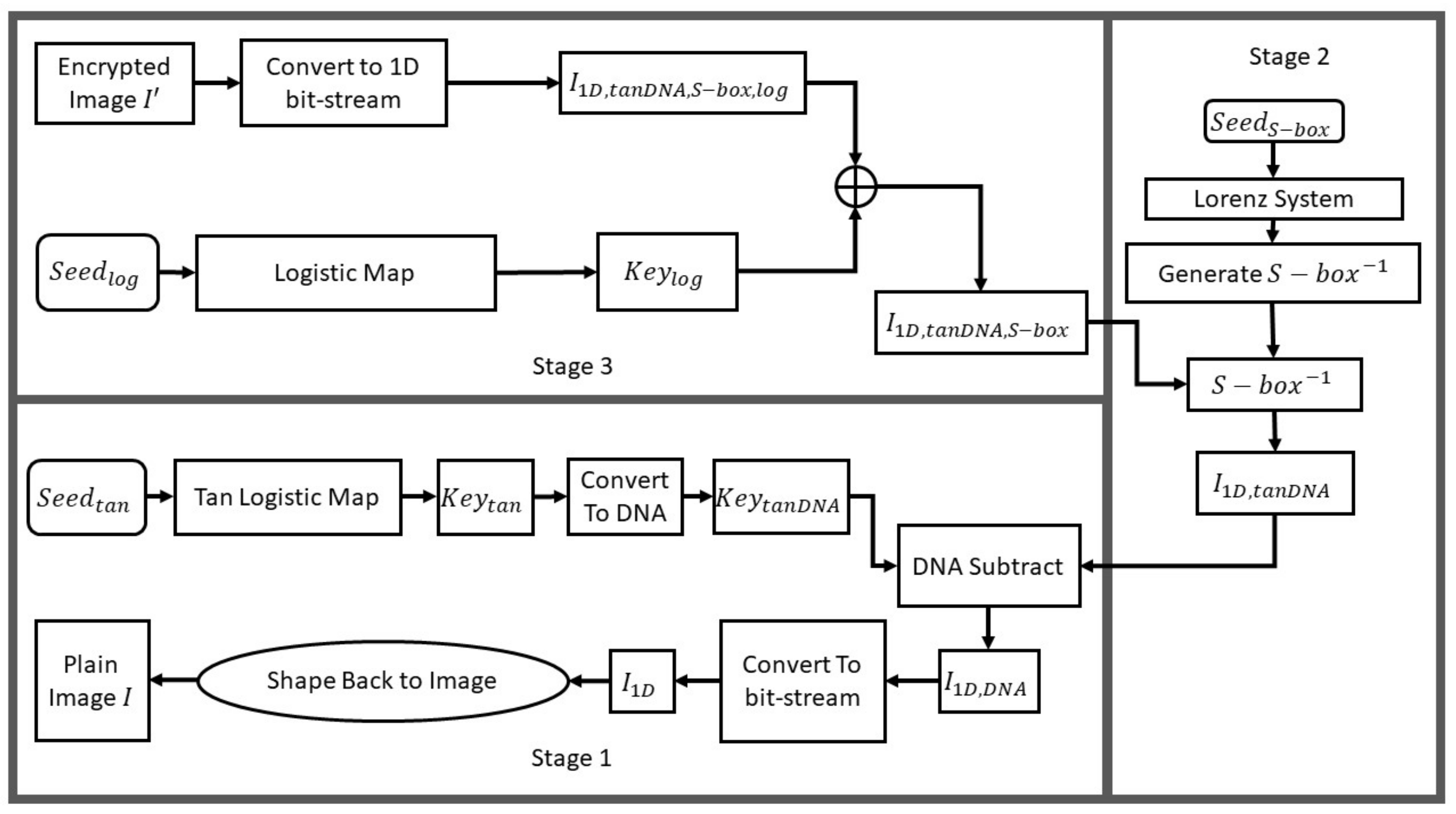
  • We propose a 3-stage image encryption scheme that makes use of Shannon’s ideas of confusion and diffusion. In the first stage, DNA coding is employed, providing diffusion at the bit level. In the second stage, an S-box based on the numerical solution of the Lorenz differential equations and a linear descent algorithm is developed and used for confusion at the pixel level. In the third stage, the logistic map is utilized to produce an encryption key, providing diffusion at the bit level. The concatenation of these three stages guarantees output encrypted images to be completely asymmetric to their original (plain) counterparts.
  • We propose an efficient and fast encryption scheme, with images of dimensions 128 × 128 encrypted in only 0.377145 s, achieving an average encryption rate of 1.015   Mbps.
  • We propose a multi-stage image encryption scheme. Using more than one encryption stage provides security against known plaintext attacks.
  • We propose an image encryption scheme that possesses a large key space of 2 372 , and is effectively resistant to brute force attacks.
  • We utilize both conventional (information entropy, pixel cross-correlation, MSE, PSNR, MAE, NPCR, UACI and NIST SP 800 suite) and unconventional performance evaluation metrics such as the Fourier transform and advanced bit dependency metrics to gauge the security and robustness of the proposed cryptosystem.
This paper is organized as follows. Section 2 outlines the mathematical background and describes the proposed image cryptosystem. Section 3 presents the computed numerical results and carries out a comparative analysis with counterpart cryptosystems from the literature. Finally, Section 4 draws the conclusions and suggests possible future research directions.

2. Proposed Image Cryptosystem

This section describes the proposed 3-stage image cryptosystem. It starts off by describing each stage separately, then how they complement each other forming one cryptosystem. Finally, the decryption process is described.

2.1. DNA Encoding Based on a Tan Variation of the Logistic Map

As mentioned before, key embedding is considered as a critically important component in image encryption. This is due to the role it plays in data diffusion. Moreover, in many of the more recent image encryption techniques, key embedding is performed two times, separated by a confusion step. As the proposed technique in this work follows the same model, the two stages of key embedding are performed differently. The third stage in this work utilizes bit-wise key embedding, as discussed in Section 2.3. For the first stage, which is the scope of this section, DNA encoding is utilized as a means for embedding a seed-based key into the raw data of an input image (to be encrypted), which is demonstrated in Section 2.1.2. Prior to that, the method of the key generation is discussed as well in Section 2.1.1.

2.1.1. Tan Variation of the Logistic Map

The logistic map is a recurrence relation, which is also a second-degree polynomial mapping that models how complex, chaotic behavior can be simulated by extremely simple non-linear dynamic equations. In recorded research history, the first mention of an equation which behaves accordingly dates back to 1976 [41]. The general mathematical definition of a logistic map is (Equation (3) in [41]):
X t + 1 = α × X t × ( 1 X t )
Equation (1) shows a recurrent function where the value of X t + 1 is directly calculated using the value of X t , and the value of a scale factor α . Adopted in this work is a variation of the logistic map function, which utilizes the application of the tan function, beside introducing the use of a seed (as the value of X 0 ). The tan variation is equated as:
X t + 1 = α × t a n ( X t ) × ( 1 X t )
Regarding the ranges for both keys ( α and X 0 ), both are to be chosen such that for every X t in the sequence, the range should remain ] 0 , 1 [ . Starting by the lower limit, the 0 is avoided as t a n ( 0 ) = 0 , which will result in, once a 0 appears in the sequence, all remaining values in the sequence will become 0. When it comes to the upper limit, given that the function in a tan variant, π 2 1.5708 is to be avoided as t a n ( π 2 ) = . Moreover, plotting the tan curve, starting from 1 till 1.5708 , the curve slope starts to be steep (in other words, with a tangent slope greater than 1). The main effect of this is that the rate of increase in tan values, given small steps in input, starts to be harder to limit (as it approaches infinity). As per that, initiating the value of X 0 , the range is considered optimal (for this scenario) as ] 0 , 1 [ . According to the X 0 range, regarding the scale factor α , for a chaotic behaviour, the range is [ 3.3 , 3.6 ] . This is confirmed visually through plotting the bifurcation diagram and Lyapunov exponent, in Figure 1 and  Figure 2, respectively.

2.1.2. DNA Encoding

Numerous studies have identified the DNA computer characteristics of vast parallelism, enormous storage, and ultra-low power consumption. DNA cryptography is a novel cryptography discipline that evolved from research on DNA computing, in which DNA is employed as an information carrier and contemporary biological technology is used as an implementation tool. As per that, in order to achieve better encryption, the DNA domain is the domain variation on which the image will be manipulated during this stage. The process of DNA encoding of an image is a modification of the bit stream representation in which each pair of successive bits is joined. In such a situation, the processes conducted would seem to be bit-level operations, but the attacker would not be able to readily trace them back using bit-level analyses.
DNA coding has three stages. First, it creates a DNA sequence from bit stream sequences by merging every 2 bits into 1 DNA base, as per the following relation:
{ ( 00 A ) , ( 01 T ) , ( 10 C ) , ( 11 G ) } .
Note that other relations also exist [21]. Table 1 shows eight possible permutations of complementary DNA encoding and decoding.
Second, applying a DNA level procedure. As reversibility is required, in this work, addition and subtraction are the inverse operations of choice, which are performed according to Table 2. In the last phase, a DNA sequence is converted into a bit stream.
The stated approach requires a DNA sequence of the same length as the image-generated DNA sequence in order to finish the encryption process. This work generates a PRNG seed-based bit stream, which is subsequently transformed into a DNA sequence. Given the two sequences (image and seed), the aforementioned processes may be carried out, with addition being used for encryption and subtraction for decryption. Figure 3 illustrates an example DNA sequence.

2.2. Lorenz S-Box

An S-box is a vital non-linear component of any image encryption system. This is because it takes advantage of Shannon’s property of confusion [42]. For the formation of the S-box, a PRNG building approach is applied. In other words, a random sequence is initially produced (using a seed since reconstruction is required), and then employed as a sequential selection factor until the S-box is completely constructed. For the production of PRNG sequences, the Lorenz system is used. The Lorenz system is a mathematical model for atmospheric convection. It was developed in 1963 by Edward Lorenz [43]. The mathematical model for this system is defined by the following three partial differential equations (where σ , ρ , and β are provided as seeds):
d x d t = σ ( y x ) ,
d y d t = x ( ρ z ) y ,
d z d t = x y β z .
The Lorenz system is numerically solved, resulting in a 3D geometry, as shown in Figure 4. Next, the x, y, and z coordinates of each point in the solution are flattened into a single 1D array, which is then turned into a bitstream using the median of the list as a threshold. Finally, each 8-bits are used to form a decimal number ϕ [ 0 , 255 ] . For example, using the values σ = 10 , β = 8 / 3 , and ρ = 28 , we obtain the first eight bits in the generated bitstream as { 1 , 1 , 1 , 0 , 0 , 1 , 0 , 0 } , which we convert into a decimal value of 228, as shown in the first entry of the S-box in Table 3.
Given a series S of 256 numbers (unsorted and containing repeated numbers), the S-box is constructed in constant time using the procedures of Algorithm 1.
Algorithm 1Generate S-box given S and L
1.
L = [ 0 255 ]
2.
n = 0
3.
i = S n % L e n g t h ( L )
4.
append L [ i ] to S-box
5.
delete L [ i ] from L
6.
n = n + 1
7.
if n < = 256 : G o T o ( 2 )
As an example, given seed values of σ = 10 , ρ = 28 , and β = 8 / 3 , the generated S-box is as shown in Table 3.

2.3. The Logistic Map

The logistic map, as a 1D chaotic function, is a nonlinear deterministic system. It contains a variety of attributes, including strong sensitivity to initial conditions (used for seed effect modeling), and deterministic behavior (used for sequence reconstruction). Chaotic sequences generated by dynamical functions are pseudo-random sequences with very complicated and difficult to anticipate features. Therefore, chaotic systems may increase an encryption system’s security. In the third stage of the proposed encryption approach, we make use of the logistic map, expressed mathematically as in (1), where two variables govern the function’s behaviour. The first variable is the scale factor, α [ 3.7 , 4 ] , representing the rate of change of the returned data. The second variable is the initial value X 0 [ 0 , 1 ] , determining the starting point of the graph.

2.4. Proposed Cryptosystem

The encryption procedure may be broken down into three (distinct) subroutines since it uses a 3-stage encryption approach. Each of the subroutines receives its own individual set of parameters (an image and a seed) and produces mostly only one result (encrypted image). In addition, each one is equipped with a reverse subroutine, which is essential for the decryption process. In Section 2.4.1 and Section 2.4.2, the sequential procedures of both encryption and decryption processes are demonstrated, respectively.

2.4.1. Encryption Procedure

The encryption procedure, as mentioned, is divided into three stages. Each stage represents the interaction between the input image, and the seed-based key involved, in order to result in the final output, which is the encrypted image. Moreover, each stage is performed over multiple steps. For elaboration, this procedure can be enumerated in the following steps:
1.
Stage 1: DNA Encoding Based on a Tan Logistic Map.
(a)
As a start, the input image, I of dimensions M × N , is converted into a 1D bit-stream to produce I 1 D , alongside calculating the length of this bit-stream:
B i t S t r e a m L e n g t h = M × N × 24
(b)
Given a seed for the Tan variation of the logistic map, which consists of values for both X 0 and α , a sequence of numbers is generated ( S e q t a n ) using (2), which is equal in length to the bit-stream length.
(c)
Forming the K e y t a n , the median ( m i d ) of the sequence is generated, and each element is compared against this median value, converting the sequence into a bit-stream (comparing with the median value assures producing an equal number of 0’s and 1’s in the bit-stream, without sacrificing the PRNG aspect.) This step is performed as per the following equations:
C ( n ) = 1 , n > m i d 0 , o t h e r w i s e
K e y t a n = i = 0 B i t S t e a m L e n g t h C ( S e q t a n )
(d)
Both bit-streams I 1 D and K e y t a n are converted into DNA-streams using (3), generating I 1 D , D N A and K e y t a n D N A , respectively.
(e)
Both DNA-streams are then added, using Table 2, generating I 1 D , t a n D N A , then converted back into a bit-stream, as per the following equation:
I 1 D , t a n D N A = A d d D N A ( I 1 D , D N A , K e y t a n D N A )
2.
Stage 2: S-box Application.
(a)
Given a seed for the S-box, which consists of the Lorenz system inputs, σ , β , and ρ , the Lorenz system is calculated (as in Figure 4), then converted into a 1D sequence using (11) (as in Figure 5) of length 2048 (to form 256 numbers, 8 bits each).
L o r e n z 1 D = { P 1 , P 2 , , P M } { x 1 , y 1 , z 1 , x 2 , y 2 , z 2 , , x M , y M , z M } .
(b)
As performed with the tan sequence, the median value will be utilized in combination with (8) in order to convert the Lorenz 1D sequence into a bit-stream. Then, each 8 bits are further converted to decimal, resulting in a list S [ 0 , 255 ] , and | S | = 256 .
(c)
List S is provided as input to Algorithm 1, producing the S-box. Finally, the S-box is applied as:
I 1 D , t a n D N A , S b o x = S b o x ( I 1 D , t a n D N A )
3.
Stage 3: Logistic Map Encoding.
(a)
Given a seed for the logistic map (Section 2.3), which consists of values for both X 0 and α , a sequence of numbers is generated ( S e q l o g ) using (1), which is equal in length to the bit-stream length of the image ( B i t S t e a m L e n g t h ).
(b)
As performed with the tan sequence (Stage 1, step c), the median value will be utilized in combination with (8) in order to convert the sequence into a bit-stream, generating K e y l o g .
(c)
The produced bit-stream, alongside the one produced the by the end of Stage 2 ( I 1 D , t a n D N A , S b o x ), an XOR operation is performed as follows:
I 1 D , t a n D N A , S b o x , l o g = I 1 D , t a n D N A , S b o x K e y l o g ,
After performing the 3 stages, reshaping I 1 D , t a n D N A , S b o x , l o g back into a 2D image (of dimensions M × N ) results in the encrypted image I . Figure 6 demonstrates a flowchart for the encryption procedure.

2.4.2. Decryption Procedure

As the reverse of the encryption procedure, decryption can be regarded as the procedure of unraveling encryption layers in order to retrieve the input image back. Hence, the previously mentioned steps are to be performed in a regressive order (as order of stages), in an inverse manner (as inverse of each performed process). Therefore, the decryption process starts with the encrypted image I , alongside the seeds ( S e e d t a n , S e e d S b o x and S e e d l o g ). Since the process of generating keys out of seeds is performed exactly the same way as in the encryption process ( K e y t a n using S e e d t a n , S b o x using S e e d s b o x , and K e y l o g using S e e d l o g ), the decryption steps elaborated next are discussed in terms of keys instead of seeds. The decryption process is procedure as follows:
1.
Stage 3: Logistic Map Encoding.
(a)
Image I of dimensions M × N , is converted into a 1D bit-stream to reproduce I 1 D , t a n D N A , S b o x , l o g .
(b)
Given I 1 D , t a n D N A , S b o x , l o g , and K e y l o g , to retrieve I 1 D , t a n D N A , S b o x , an XOR operation is performed, as follows:
I 1 D , t a n D N A , S b o x = I 1 D , t a n D N A , S b o x , l o g K e y l o g .
2.
Stage 2: S-box Application.
(a)
Given S b o x , the inverse S b o x is calculated, namely S b o x 1 .
(b)
The inverse S-box is applied as:
I 1 D , t a n D N A = S b o x 1 ( I 1 D , t a n D N A , S b o x )
3.
Stage 1: DNA Encoding Based on a Tan Logistic Map.
(a)
The bit-stream I 1 D , t a n D N A is first converted into a DNA sequence using (3).
(b)
In order to retrieve I 1 D , K e y t a n D N A is to be subtracted from I 1 D , t a n D N A using Table 2, as shown in the following equation:
I 1 D = S u b t r a c t e d D N A ( I 1 D , t a n D N A , K e y t a n D N A )
Finally, I 1 D is to be reshaped back into a 2D image (of dimensions M × N ) resulting in the input image I. Figure 7 demonstrates a flowchart for the decryption procedure.

3. Numerical Results and Performance Evaluation

An encryption algorithm’s performance is evaluated by how well it can withstand various visual, statistical, entropy, differential and brute-force attacks. In this section, the suggested image encryption algorithm’s numerical findings are presented and discussed along with a comparison to counterpart algorithms from the literature. The various analyses were run on Wolfram Mathematica® v.13.1. The utilized computer had the following specifications: 2.9 GHz Intel® CoreTM i9, 32 GB. For the sake of these tests, values used as keys for the experimental encryption process are assigned as follows: σ = 10 , β = 8 / 3 , ρ = 28 and X 0 = 0.5 . Multiple images that are commonly used in image processing applications and experimentation were utilized, all of dimensions of 256 × 256 , unless otherwise stated. The performed tests are:

3.1. Visual and Histogram Analysis

In Figure 8, Figure 9, Figure 10, Figure 11 and 
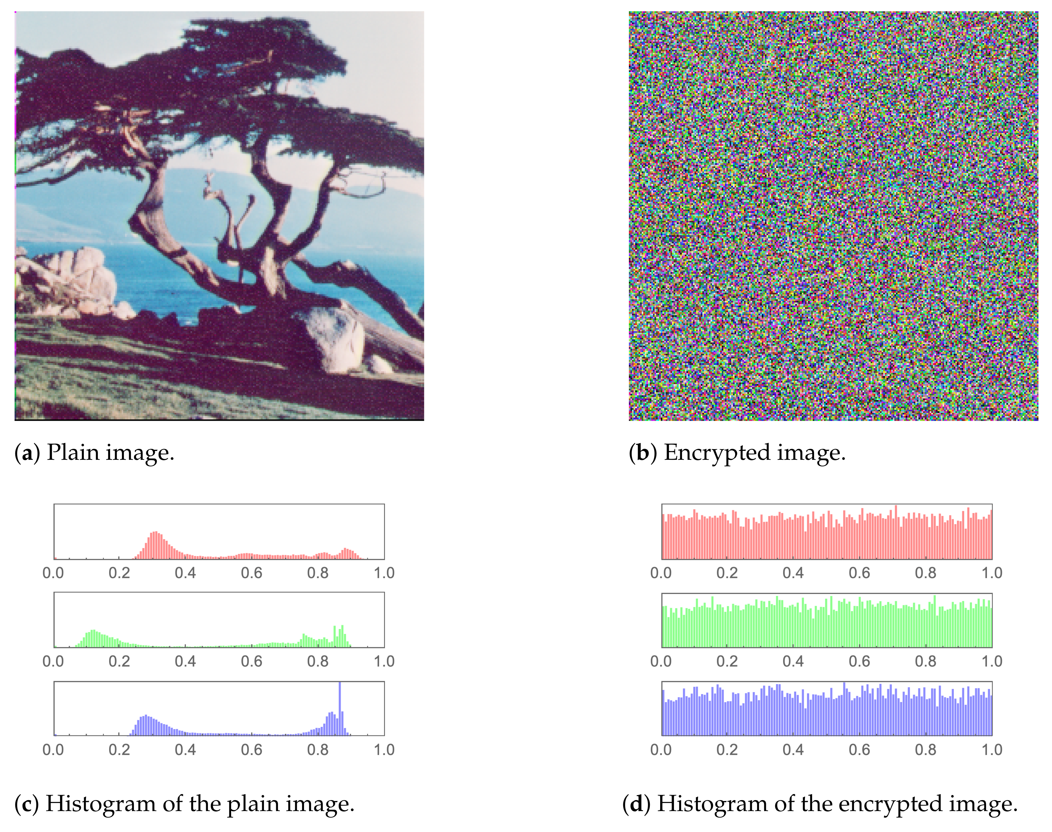
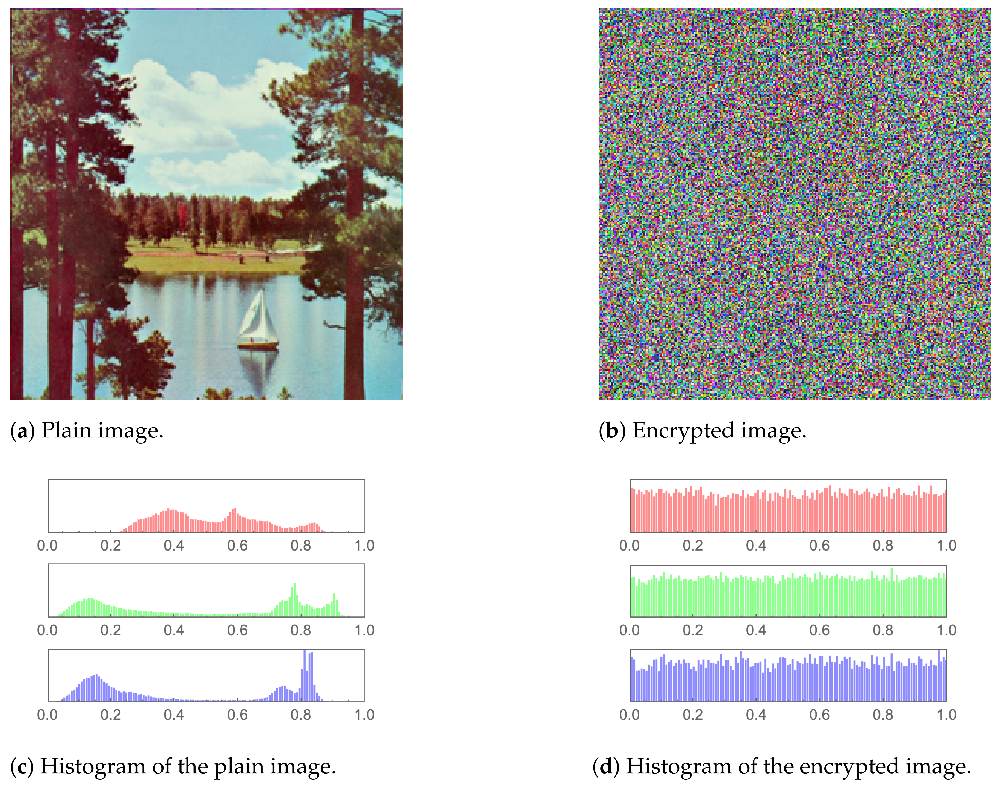
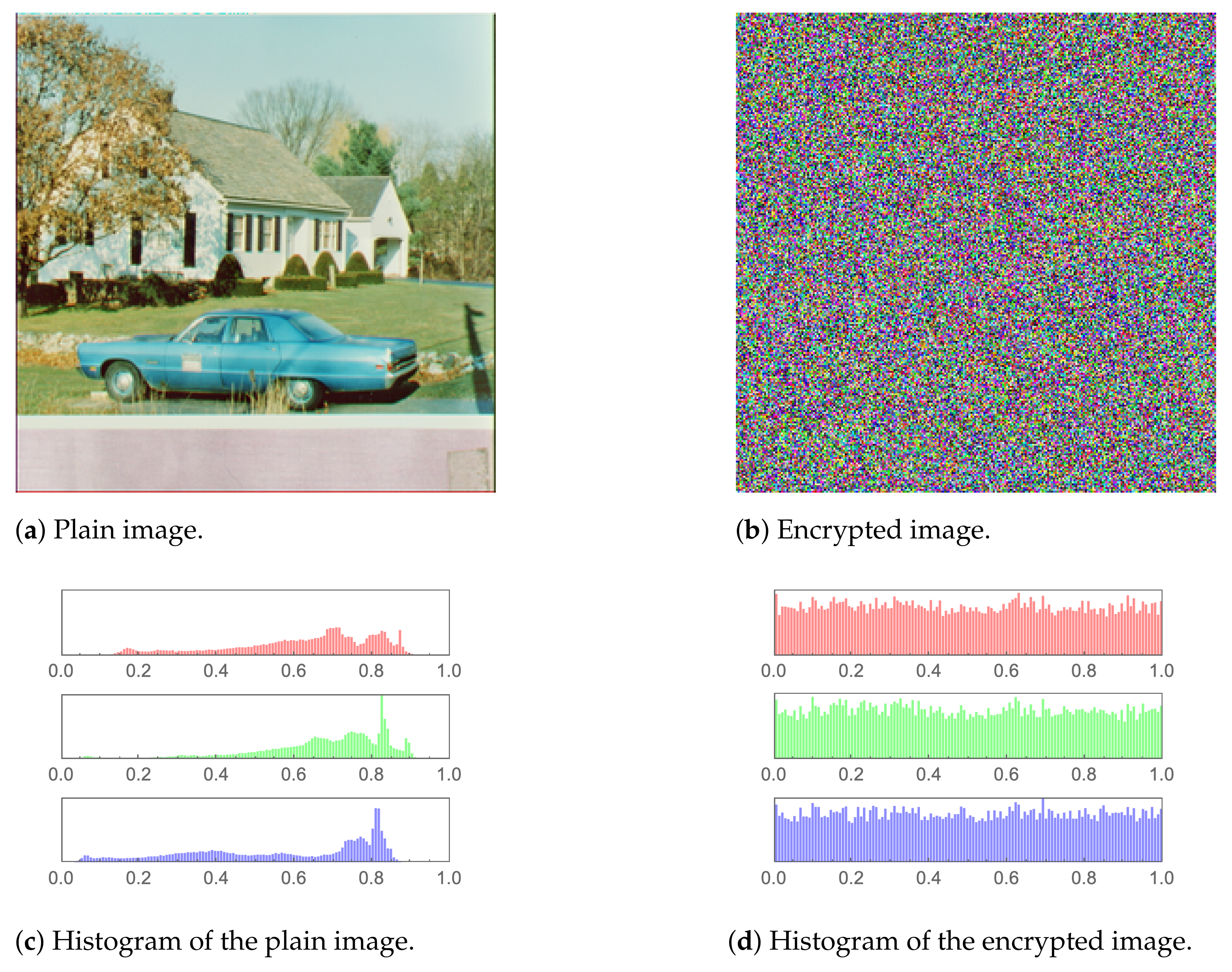
Figure 12 (including sub-figures), a number of input plain images, their encrypted forms along with their respective histograms, are shown. It is evident that the encrypted images’ pixels are asymmetric. This results in the encrypted images being distorted to a high level, to the extent that all visual features in an input (plain) image being totally absent from the encrypted one.
Moreover, histograms of the encrypted images are demonstrated as well. As the histogram of an image displays the frequency distribution of the pixels, the histogram of an encrypted image must be homogeneous to have a reliable encryption method. The core reason behind that is that a uniform histogram distribution reveals that each of the image’s gray levels has a probability that is essentially equivalent. Therefore, the image will be more robust to statistical attacks as a result.

3.2. Mean Squared Error

The Mean Squared Error (MSE) is one of the most common tools used in evaluating the similarity between two sets of numbers (in the most general form). As a variant of the Sum of Squared Differences (SSD), the same properties are inherited. For further elaboration, given two sets S and S of same size n, the SSD is calculated as follows:
S S D = i = 1 n ( S i S i ) 2 .
In light of this representation, there are three main operations performed: subtraction, squaring and summing. Subtraction is mandatory as the operation desired revolves around detecting differences. Consequently, subtraction, as a mathematical operation, produces two results: direction and magnitude. As global difference (as over the whole set) is required, differences in opposing directions are to be added up (instead of cancelling each other out). Performing that, the importance of directional differences among corresponding individual elements in both lists is neglected. Mathematically, either absolute values (retaining the magnitude) or squared values (amplifying the magnitude) are used in order to remove the polarity, which is the main difference between the Sum of Absolute Differences (SAD) and the Sum of Squared Differences (SSD). Finally, summation allows all individual elements in the list to contribute (equally) to the final result, achieving a calculation of the global perspective.
In case of the MSE, the mathematical representation is modified to the following:
M S E = i = 0 M 1 j = 0 N 1 ( I ( i , j ) I ( i , j ) ) 2 M × N .
Given two images I and I of dimensions M × N , as images rectangular areas, two-dimensional summing is required. (Each dimension of the summation is starting at 0 ( i = 0 and j = 0 ), and ending by M 1 and N 1 assuming the image (as a 2D array) is zero-indexed.) What can be perceived as a considerable alteration to the SSD is the division by the image dimensions. Such a step is performed in order to facilitate the comparison between MSE values in which image pairs’ dimensions are different. For example, I 1 and I 1 are both of size 256 × 256 with Mean Squared Error M S E 1 (both images must be of the same size). Comparing M S E 1 to M S E 2 which is calculated for I 2 and I 2 of dimensions 512 × 512 is meaningful as both values are normalized with respect to images’ scales. This entails that MSE can be preserved as the average error (in terms of SSD) per pixel, given two images.
In the scope of this work, MSE is evaluated for input images and their encrypted counterparts. In such a case, the ideal value for a well-performing encryption technique is expected to be high. In other words, as the target of encryption is to distort the visual attributes of images, the similarity should be minimal, resulting in a maximal error factor. Table 4 shows the computed MSE values for various input image examples, alongside showcasing how these values stand in comparison to other encryption techniques in the literature, demonstrating comparable results.
It is common practice to report MSE and Peak Signal to Noise Ratio (PSNR) values together when analyzing image encryption algorithms. This is because the computation of PSNR is based on the value of MSE. However, the authors of [39,40] only provide PSNR values in their respective works, with no mention of MSE values. This explains why Table 4 displays columns of N/A under the headings of [39,40].

3.3. Peak Signal to Noise Ratio

Based on the MSE discussed in Section 3.2, PSNR, given a signal, aims at relating the error margin (represented by MSE), with respect to the peak value in the signal. In the scope of this work, the peak signal value is evaluated as the maximum pixel intensity in a given image. Accordingly, given image I, PSNR is equated as:
P S N R = 10 log I m a x 2 M S E ,
such that I m a x is the maximum pixel intensity in I. Due to the fact that MSE is SSD based (which indicates that MSE is calculated to a squared order of magnitude), I m a x is necessarily squared.
As shown in (19), PSNR in inversely proportional to MSE. Such mathematical representation steers the preference of the PSNR to be the inverse of the preference of MSE, hence a minimal value is more ideal. Table 5 presents the calculated values for the proposed cryptosystem as well as those of counterpart algorithms from the literature. In terms of MSE and PSNR, the proposed cryptosystem is shown to be superior to [16,18,26,39,40], but inferior to [17].

3.4. Mean Absolute Error

Building on the argument presented in Section 3.2, an alternate technique to Sum of Squared Differences, SSD, would be Sum of Absolute Differences, SAD. In such alternative, the task of eliminating the polarity of the per-pixel error is performed by the absolute operation instead of the square one. Therefore, parallel to the SSD equation (Equation (17)), SAD is equated as:
S A D = i = 1 n | S i S i | .
As discussed before in Section 3.2, the role of squaring, beside eliminating polarity, is to amplify the magnitude. On the other hand, using the absolute instead maintains the linearity of the behaviour of the error distribution among pixels, which is accordingly maintained in the global perspective of the whole image.
Upon such variation in the core function, MAE is represented mathematically as:
M A E = i = 0 M 1 j = 0 N 1 | I ( i , j ) I ( i , j ) | M × N ,
for two images I and I . As per this work (similar to the MSE scenario), MAE is evaluated for input images and their encrypted images. Moreover, for a well-performing encryption technique, MAE value is preferred to be maximal. Table 6 presents the numerical results of performing the MAE test on three images (Lena, Peppers, and Mandrill) in comparison to counterpart algorithms from the literature. As the numerical results demonstrate, the proposed algorithm fares comparably to them.

3.5. Information Entropy

In the domain of gray-scale images, information entropy is employed to measure the randomness of the distribution of gray pixel values of an image. According to Shannon’s theory, information entropy is calculated as:
H ( m ) = i = 1 M p ( m i ) log 2 1 p ( m i ) ,
where p ( m i ) refers to the probability of occurrence of symbol m, while M represents the total number of bits for each symbol. With respect to images, as a gray scale image has 256 different values [ 0 255 ] , which are 2 8 different possible permutations, the entropy value of an encrypted image at greatest evaluations approaches 8. Therefore, information entropy can be used to evaluate the degree of randomness of encrypted images. Entropy values of the proposed algorithm for the the images displayed and tested in this paper, along with counterpart algorithms from the literature are displayed in Table 7. The computed entropy values for the various images are very close to the ideal value of 8, which means that the proposed algorithm is resistant to entropy attacks. Furthermore, the differences across entropy values of the various cryptosystems is shown to be diminutive.

3.6. Fourier Transformation Analysis

In order to showcase the co-relation among pixels before and after encryption, the application of the Fourier transformation (for both images) is utilized, more accurately, for Discrete Fourier Transform (DFT). The main aim is, in the frequency domain, visual features such as edges and regions (which are not easily definable in the spatial domain) separate into different frequency ranges. This facilitates visual analysis and comparisons of images. Such separation takes place as a result of the interaction between the pixels in the spatial image with the increasing frequencies of the sine and cosine waves. Aiming towards transforming a spatial domain image into the frequency domain, the following Fourier transformation equation is used:
F ( k , l ) = i = 0 N 1 j = 0 N 1 f ( i , j ) e i 2 π ( k i N + l i N ) ,
such that f ( a , b ) is the image representation in the spatial domain, with the exponential term being the basis function that corresponds to each point F ( k , l ) in the Fourier space.
Interpreting a Fourier transformation of an image (presented as 2D data), two main regions of high relevance are to be looked at [46]. The first region is the middle area of the 2D grid of the Fourier transformed image. The main significance of this area is that it represents the amount of pixels with high similarity in values on the pixel level. Therefore, if a Fourier transformation image is generated out of an image with large regions (flat, same color areas), it is expected for the middle area to contain high values.
The second region is the center row, column and alongside diagonals of the Fourier transformed image. This is due to their representation of vertical, horizontal, and diagonal edges in the input image, respectively. (The Fourier image is considered to be a transposed matrix of the input image.) Thus, if the input image includes only vertical edges, the Fourier transformed image is expected to have a bright middle row, and vice versa. The rest of the Fourier transformed image represents the other features existing in the input image.
Conclusively, for a naturally looking image with wide regions and profound edges (Peppers in this example), the resulting Fourier transformed image contains a bright plus sign at its center, as observed in Figure 13b. On the other hand, on a distorted (encrypted) image, an equal description of values in the Fourier transformed image is expected due to the lack of profound regions or edges, as shown in Figure 13e.

3.7. Correlation Coefficient Analysis

In this evaluation method, the consistency of a single image is evaluated. The aim of such evaluation method is to assess (or provide an estimated coefficient for) the cohesion of near-proximity pixels. In other words, correlation coefficient analysis, in the domain of images, aims at calculating the percentage of the uniform regions with respect to the edge transitions. Hence, in a normal image case, a relatively high correlation coefficient value is expected, as it consists more of regions than edges (in terms of pixel count). On the other hand, as high distortion is aimed for in encrypted images, a smaller correlation coefficient is anticipated for it.
For mathematical evaluation, the correlation coefficient is calculated through the following equations:
ρ ( x , y ) = c o v ( x , y ) σ ( x ) σ ( y ) ,
where:
c o v ( x , y ) = 1 N i = 1 N ( x i μ ( x ) ) ( y i μ ( y ) ) ,
σ ( x ) = 1 N i = 1 N ( x i μ ( x ) ) 2 ,
μ ( x ) = 1 N i = 1 N ( x i ) .
Starting by the mean average of each distribution as in (27), two distribution behaviours are measured. The first behaviour is the dispersion (using (26)), which represents the uncertainty of the distribution. The second behaviour is the covariance (using (25)), which evaluates the linear direction similarity. Combining both mathematical phenomenons results in reaching an evaluation for the correlation coefficient, represented in (24).
As previously mentioned, for a normal image (the input), a high correlation value is expected. On the other hand, a highly distorted image would result in having a low correlation coefficient. Table 8 demonstrates performing the correlation coefficient analysis on three images (Lena, Peppers and Mandrill), for both images, input and encrypted. Moreover, as the covariance is a directional relation, the three main directions are calculated, which are horizontal, vertical and diagonal. As shown by the numerical results, the input image showed a value approaching 1 in all cases, while the encrypted showed a value approaching 0. Table 9 presents the comparison between the proposed approach and counterpart algorithms from the literature, which showcases nearly similar results. Moreover, Table 10 and Table 11 show the results of numerical comparison among the proposed algorithm and its counterparts from the literature, focusing on the color channels separately, with respect to the three directions for the images Lena and Mandrill, respectively.
Alongside the numerical analysis provided by (24), directional covariance can be visualized by the plotting of the co-occurrence matrix. In case of images with natural visual aspects (more pixels representing homogeneous regions than transitional edges), values of high similarity tends to co-exist with a higher probability, resulting in a mostly linear distribution of magnitudes within the matrix. Oppositely, in a highly distorted (encrypted) image, a more equal distribution of values is expected to take place instead. For demonstration, this is carried out in Figure 13, where Figure 13c is for the plain image, while Figure 13f is for its encrypted version. It is clear that the 3D plot for the plain image is diagonal in nature, unlike that of the encrypted image, which resembles a mountain in 3D space, as expected for an encrypted image, signifying random pixel locations. For further demonstration, focusing on the Papers image, Figure 14, Figure 15 and Figure 16 show 3D plots of the co-occurrence matrices for the red, green and blue color channels, respectively. As demonstrated, pixel correlations are fully distorted on each color level individually.

3.8. Differential Attack Analysis

In this section, the quality of image cryptosystems is judged on the grounds of the direct difference between the input and the encrypted images. In other words, the input image is directly compared with the encrypted on pixel by pixel, or mean average bases. Such evaluation is performed in order to calculate a numerical percentage showcasing the difference in color intensities (per pixel, or as a mean average) taking place as a result of the encryption process. According to the fact that the lack of similarity among corresponding pixels within both images is encouraged, such pixel by pixel evaluation is necessarily performed. Moreover, a more global perspective of the cumulative pixels change rates among images (presented in the mean averages) is evaluated, which denotes the existence of general color intensity similarity among these images. In the literature, two tests are most commonly performed to fulfill these test aspects: NPCR for pixel by pixel comparison, and UACI for the mean average difference evaluation.
Number of pixels changing rate (NPCR) represents the percentage evaluation of the amount of changed pixels. The difference between pixels is performed with a strict equality perspective. Given two images I 1 and I 2 (of dimensions M × N ), the difference per pixel D ( x , y ) (where x and y are the coordinates of the pixel) is calculated as:
D ( x , y ) = 0 I 1 ( x , y ) = I 2 ( x , y ) 1 O t h e r w i s e x [ 1 , M ] & y [ 1 , N ]
Accordingly, NPCR is equated as:
N P C R = x = 1 M y = 1 N D ( x , y ) M × N × 100 .
As per this representation, a higher percentage denotes larger difference between the two images. As a large difference is desired, in the literature, 99 % is the target NPCR score for a good encryption technique.
In another perspective, the unified average change intensity (UACI) evaluates the difference between two images in terms of the mean averages. Mathematically, UACI is equated as:
U A C I = 1 M × N x = 1 M y = 1 N | I 1 ( x , y ) I 2 ( x , y ) | 255 × 100 .
In the literature, a target percentage of more than 33 % denotes a strong encryption technique. (With respect to the color range [ 0 , 255 ] , 33 % is approximated to 85 steps of difference in intensity.)
Table 12 shows the result of performing NPCR and UACI, comparing the input and the encrypted image generated by the proposed algorithm, using various images as inputs. (As discussed before, the NPCR is greater than 99.6 % and the UACI should also be greater than 33 % .) For these tests, the proposed algorithm is also compared with its counterparts from the literature, as shown in Table 13 and Table 14. As shown, the computed NPCR value of the proposed algorithm is > 99 % in all cases. On the other hand, the UACI value did not meet the optimal value. However, the exception to this case is the Girl image, which resulted in 32.1283 , 36.4526 , and 37.4855 for color channels red, green and blue, respectively, alongside 35.3554 as an overall.

3.9. The National Institute of Standards and Technology Analysis

The National Institute of Standards and Technology (NIST) SP 800 analysis is a set of statistical tests which ensure the necessary cryptographic properties of the random number sequences are met. The encrypted images’ equivalent binary stream are run through the NIST analysis. To ensure resilience to cryptographic attacks, the results ought to surpass a p-value of 0.01 . Table 15 shows the outcome of running the analysis. The results reflect the cryptographic robustness of the proposed scheme, with all the tests’ outcomes larger than 0.01 . Hence, we can safely conclude the validity of our proposed cryptosystem.

3.10. Key Space Analysis

Key space analysis is calculated as the Cartesian product of the domains of the key values involved in the encryption procedure. Such a step is carried out in order to compute the amount of unique keys that can be utilized in the encryption procedure, which accordingly results in creating various possible encryption instances for the same input image. In the proposed image encryption algorithm, there is a total of seven variables involved in a single encryption procedure. The first two variables are used (in the first stage Section 2.1) for the generation of the bit-stream using the tan variation of the logistic map, which is used in the DNA encoding, namely α and X 0 . In the second stage (Section 2.2), a Lorenz system is used for the S-box generation, which demands three variables ( σ , ρ and β ). Finally, in the last stage discussed in Section 2.3, two keys are used, which are r and t r ( 0 ) . As the largest machine precision is 10 16 , the key space is about 10 7 × 16 = 10 112 2 372 , which exceeds the threshold earlier proposed in [61] as 2 100 . This means that our proposed scheme can resist brute–force attacks. Furthermore, an examination of key space values of related image encryption schemes from the literature, as in Table 16 indicates that the proposed scheme utilizes a comparably much larger key space than most of its counterparts. The only exception here being the work of [39], in which one of the encryption stages relies on the random movement of a chess piece (Castle), which results in a very large key space.

3.11. Histogram Dependency Tests

According to the aim of image encryption (distorting image details in a reversible manner), all forms of correlation between the plain image and its encrypted version is to be absent. In such a test scenario, the images (plain and encrypted) are evaluated on the histogram level. Moreover, these tests are performed on the image as one unit, as well as on the color channels separately. Therefore, given two histograms of images, the comparisons performed aims at evaluating the level of the linear dependency between them. As any dependency (as a form of correlation) test evaluates the level of association between two variables [67], in a well performing encryption technique, the dependency level should be as low as possible. Accordingly, calculating the dependency coefficient as a value in the range [ 1 , 1 ] , it is desirable to be as close to 0 as possible (where 1 means strong dependency, and −1 means strong inverse dependency). In other words, given two distributions, dependency between them is evaluated as the alignment of one with respect to the other, which is either both are following the same linearity (evaluating to 1), or following perpendicular linearity (evaluating to 1 ), or there is no linearity (evaluating to 0). As mentioned, in the context of this work, the pair distributions of variables to evaluate are the histograms of both the input and the encrypted images. Out of many dependency evaluation techniques, in this work, five tests are performed, namely: Blomqvist β , Goodman-Kruskal γ , Kendall τ , Spearman ρ , and Pearson correlation r [68].
As a medial correlation coefficient, Blomqvist evaluates correlation between two distributions of variables X and Y, with their medians x ¯ and y ¯ , respectively, as per the following Equation:
β = { ( X x ¯ ) ( Y y ¯ ) > 0 } { ( X x ¯ ) ( Y y ¯ ) < 0 } .
Considering the median as a reference point, pairs of elements across the two distributions of variables are either on the same side of the median (creating a linear correlation), or not (breaking the linear correlation).
Based on the relative order of succeeding elements in the two distributions of variables, the Goodman-Kruskal measure of monotonic association is used in a pairwise manner. Transforming the two histograms into one set of pairs in a 1 to 1 formation (containing pairs of the form ( H 1 ( n ) , H 2 ( n ) ) ), comparing two pairs ( ( H 1 ( i ) , H 2 ( i ) ) and ( H 1 ( j ) , H 2 ( j ) ) for example), they are either aiding the linear correlation (concordant pairs) or breaking it (discordant pairs). Counting both concordant pairs and discordant pairs provides two counts, n c and n d , respectively. Given these two counts, Goodman-Kruskal correlation is equated as:
γ = n c n d n c + n d .
Based on the same concept of concordant pairs and discordant pairs, Kendall evaluates correlation with respect to the sample size n, equating τ as follows:
τ = n c n d n ( n 1 ) 2 .
For a rank-based correlation test, Spearman rank correlation test relates the rank of an element (its position if the list was sorted), with respect to the mean rank value. Spearman rank correlation is equated as:
ρ = ( R i x R ¯ x ) ( R i y R ¯ y ) ( R i x R ¯ x ) 2 ( R i y R ¯ y ) 2 ,
where x and y are the two evaluated variables, R i l is the rank of element i in list l, and R ¯ l is the mean of ranks of l.
Finally, Pearson correlation, as the most popular and straightforward correlation technique, simply relates elements in the distributions directly to their mean averages. Pearson correlation is equated as:
r = ( X i X ¯ ) ( Y i Y ¯ ) ( X i X ¯ ) 2 ( Y i Y ¯ ) 2 ,
where X ¯ and Y ¯ are the means of the distributions X and Y, respectively.
Table 17 shows the results of performing the six tests on various images. As all scores are approaching 0, there is a very minimal dependency between the input and encrypted images in terms of histograms over all color channels.

3.12. Execution Time Analysis

Encryption and decryption times are used to determine an algorithm’s complexity and suitability for real-time applications. Table 18 displays those values for the Lena image at various dimensions, N × N , where N { 64 , 128 , 256 , 512 , 1024 } . Depending on the image dimensions, the overall encryption and decryption time varies from 0.228822s, for N = 64 , to just under a minute, for N = 1024 . In addition, Table 19 presents a comparison of the encryption time among the proposed algorithm and its counterparts from the literature. Note that the differences in encryption time depend on numerous factors, including the algorithm’s complexity, the machine specifications on which the algorithm is executed (i.e., processing power and accessible memory), and the software package or programming language used to execute the algorithm. In this work, Wolfram Mathematica® is employed, while in [39,66,69,70,71] Mathworks Matlab® was the software of choice. The average encryption speed for the proposed scheme is 1.015 Mbps.

3.13. S-Box Performance Analysis

As a stable component, which is almost always at the core of any image encryption technique, also, as it holds the responsibility towards implementing Shannon’s property of confusion in a cryptosystem, an S-box should be evaluated in isolation from the total perspective of the whole encryption process. There are five tests most commonly performed in order to evaluate the confusion capability of an S-box. The first test is nonlinearity [72], which represents the measure of how many bits in the truth table of a Boolean function need to be changed in order to approach the closest affine function (optimal value of 120, with most commonly achieved of 112). The second test is linear approximation probability (LAP) [73], which identifies the probability of bias for a given S-box (optimal value of 0.0625). Third test is a differential approximation probability (DAP) [74], which is a technique that examines the impact of specific variations in inputs and its effect on encrypted output (optimal value of 0.0156). Fourth, are the bit independence criterion (BIC) [75], which evaluates the relation between encryption procedures and the repeated patterns in the encrypted output (optimal value of 112). Finally, strict avalanche criterion (SAC) [75], which calculates the rate of change in the encrypted output with respect to the change in the input on a bit by bit level (optimal value of 0.5).
In commonly used methods for S-box generation, the procedure followed in the process of S-box generation takes the evaluation methods into consideration. In this work, as demonstrated in Section 2.2, a PRNG approach is followed, which introduces some advantages alongside some disadvantages. The main advantage is that the overall encryption process requires more keys, increasing the overall key space, resulting in more resistance to attacks. On the other hand, as per the keys provided to the S-box generation process, the evaluation scores for each S-box generation scenario is not fixed. As per that, the relation between various keys in the key space and encrypting strengths of the generated S-boxes is to be correlated, as a future work.
Evaluating an S-box generated using keys: σ = 10 , β = 8 / 3 , and ρ = 28 (shown in Table 3) utilizing the aforementioned evaluation methods results in the findings presented in Table 20. As the evaluations demonstrate, not all optimal values were met. More precisely, while nonlinearity and SAC showed near optimal scores, DAP scored average, and LAP was far from optimal. For better reference, Table 21 shows scores comparison with popular S-boxes in the literature, which represent acceptable scores overall. These shortcomings are a natural result of the mechanism we adopted for the S-box generation, which is completely random, with full disregard to major S-box design criteria, which aim at avoiding fixed points and short ring cycles [76,77]. On the other hand, they can be regarded as trade-offs to increasing the key space of the overall encryption process, due to the addition of the new three tunability parameters ( σ , ρ and β of the Lorenz system). In other words, instead of having a fixed (well-performing) S-box as one of the encryption stages, a randomly-generated S-box will allow for increasing the number of encrypted images per a single input plain image. In the case of the proposed work, the factor of increase in encrypted images per a single input plain image is 2 19 , as thoroughly discussed in Section 3.10.

4. Conclusions and Future Works

This research work proposed a 3-stage image encryption scheme. DNA encoding, along with a tan variant of the logistic map, were made use of in the first stage of encryption. An S-box based on the numerical solution of the Lorenz differential equations and a linear descent algorithm was developed for the second stage, and utilized to carry out bit confusion. Finally, the logistic map in its original form was utilized to produce an encryption key for the third stage of encryption. Performance of the proposed image cryptosystem was evaluated utilizing commonly used metrics from the literature, as well as newly adopted ones. The computed values reflect a secure and robust cryptosystem that is resistant to visual, statistical, entropy, differential, known plain text and brute-force attacks. This has been validated through comparison with the performance of counterpart schemes from the literature. The proposed cryptosystem was shown to exhibit comparable performance to them, if not superior at times. Future works could: (a) attempt to replace the utilized 1D chaotic function with a higher-dimensional one. While this would invariably improve the security even more, it is expected that it might affect the computational complexity, and thus the execution time of the algorithm; and (b) optimize the generated S-box design, to achieve better values in all of the evaluation metrics. While the proposed S-box design did not score optimal values in all metrics, this was compensated in the proposed cryptosystem as a whole, due to the other two encryption stages. Furthermore, a future work could replace the utilization of the Lorenz system for the construction of the S-box. The reason behind such a recommendation is that the Lorenz system is a continuous one, with its computation heavily depending on the numerical method adopted in solving it. A better choice would be any discrete chaotic function.

Author Contributions

Conceptualization: M.G., I.K. and W.A.; methodology, M.G. and W.A.; software, M.G., H.Y., M.I., S.A., I.K., R.E. and W.A.; validation, M.G., H.Y., M.I., S.A. and W.A; writing—original draft preparation, M.G., E.A. and W.A.; writing—review and editing, W.A.; visualization, M.G. and W.A.; supervision, R.E., E.A. and W.A. All authors have read and agreed to the published version of the manuscript.

Funding

This research received no external funding.

Data Availability Statement

Not applicable.

Acknowledgments

The authors would like to acknowledge the time and efforts exerted by the esteemed reviewers of this manuscript, which have led to its improvement.

Conflicts of Interest

The authors declare no conflict of interest.

Abbreviations

The following abbreviations are used in this manuscript:
DNADeoxyribonucleic acid
MAEMaximum absolute error
MSEMean Square Error
NISTNational Institute of Standards and Technology
NPCRNumber of Pixel Changing Ratio
PSNRPeak Signal-to-Noise Ratio
UACIUnified Averaged Change Intensity

References

  1. El-Mahdy, A.; Alexan, W. A comparative study on the performance of LLR-and SNR-based hybrid relaying schemes. Wirel. Commun. Mob. Comput. 2017, 2017, 4063792. [Google Scholar] [CrossRef]
  2. Huang, H.; Li, J. Research on Network Communication Model and Network Security Technology through Big Data. In Proceedings of the 2021 IEEE International Conference on Data Science and Computer Application (ICDSCA), Dalian, China, 29–31 October 2021; pp. 138–141. [Google Scholar] [CrossRef]
  3. El Mahdy, A.; Alexan, W. A threshold-free LLR-based scheme to minimize the BER for decode-and-forward relaying. Wirel. Pers. Commun. 2018, 100, 787–801. [Google Scholar] [CrossRef]
  4. Elkandoz, M.T.; Alexan, W. Image encryption based on a combination of multiple chaotic maps. Multimed. Tools Appl. 2022, 81, 25497–25518. [Google Scholar] [CrossRef]
  5. El-Shafai, W.; Almomani, I.M.; Alkhayer, A. Optical bit-plane-based 3D-JST cryptography algorithm with cascaded 2D-FrFT encryption for efficient and secure HEVC communication. IEEE Access 2021, 9, 35004–35026. [Google Scholar] [CrossRef]
  6. Farrag, S.; Alexan, W. Secure 3d data hiding technique based on a mesh traversal algorithm. Multimed. Tools Appl. 2020, 79, 29289–29303. [Google Scholar] [CrossRef]
  7. Alexan, W.; Elkhateeb, A.; Mamdouh, E.; Al-Seba’Ey, F.; Amr, Z.; Khalil, H. Utilization of corner filters, aes and lsb steganography for secure message transmission. In Proceedings of the 2021 International Conference on Microelectronics (ICM), New Cairo City, Egypt, 19–22 December 2021; pp. 29–33. [Google Scholar]
  8. Alexan, W.; Mamdouh, E.; ElBeltagy, M.; Hassan, F.; Edward, P. Image Feature-Based Watermarking. In Proceedings of the 2022 International Telecommunications Conference (ITC-Egypt), Alexandria, Egypt, 26–28 July 2022; pp. 1–6. [Google Scholar] [CrossRef]
  9. Alexan, W.; Ashraf, A.; Mamdouh, E.; Mohamed, S.; Moustafa, M. Iomt security: Sha3-512, aes-256, rsa and lsb steganography. In Proceedings of the 2021 8th NAFOSTED Conference on Information and Computer Science (NICS), Hanoi, Vietnam, 21–22 December 2021; pp. 177–181. [Google Scholar]
  10. Yasser, S.; Hesham, A.; Hassan, M.; Alexan, W. Aes-secured bit-cycling steganography in sliced 3d images. In Proceedings of the 2020 International Conference on Innovative Trends in Communication and Computer Engineering (ITCE), Aswan, Egypt, 8–9 February 2020; pp. 227–231. [Google Scholar]
  11. Coppersmith, D. The Data Encryption Standard (DES) and its strength against attacks. IBM J. Res. Dev. 1994, 38, 243–250. [Google Scholar] [CrossRef]
  12. Adam, N.; Mashaly, M.; Alexan, W. A 3des double–layer based message security scheme. In Proceedings of the 2019 2nd International Conference on Computer Applications & Information Security (ICCAIS), Riyadh, Saudi Arabia, 19–21 March 2019; pp. 1–5. [Google Scholar]
  13. Daemen, J.; Rijmen, V. The Design of Rijndael; Springer: Berlin/Heidelberg, Germany, 2002; Volume 2. [Google Scholar]
  14. Moussa, Y.; Alexan, W. Message security through AES and LSB embedding in edge detected pixels of 3D images. In Proceedings of the 2020 2nd Novel Intelligent and Leading Emerging Sciences Conference (NILES), Giza, Egypt, 24–26 October 2020; pp. 224–229. [Google Scholar]
  15. Liu, X.; Tong, X.; Wang, Z.; Zhang, M. Efficient high nonlinearity S-box generating algorithm based on third-order nonlinear digital filter. Chaos Solitons Fractals 2021, 150, 111109. [Google Scholar] [CrossRef]
  16. Alexan, W.; ElBeltagy, M.; Aboshousha, A. Image Encryption Through Lucas Sequence, S-Box and Chaos Theory. In Proceedings of the 2021 8th NAFOSTED Conference on Information and Computer Science (NICS), Hanoi, Vietnam, 21–22 December 2021; pp. 77–83. [Google Scholar]
  17. Khan, M.; Masood, F. A novel chaotic image encryption technique based on multiple discrete dynamical maps. Multimed. Tools Appl. 2019, 78, 26203–26222. [Google Scholar] [CrossRef]
  18. Younas, I.; Khan, M. A new efficient digital image encryption based on inverse left almost semi group and Lorenz chaotic system. Entropy 2018, 20, 913. [Google Scholar] [CrossRef] [Green Version]
  19. Sambas, A.; Vaidyanathan, S.; Tlelo-Cuautle, E.; Abd-El-Atty, B.; El-Latif, A.A.A.; Guillén-Fernández, O.; Sukono; Hidayat, Y.; Gundara, G. A 3-D Multi-Stable System with a Peanut-Shaped Equilibrium Curve: Circuit Design, FPGA Realization, and an Application to Image Encryption. IEEE Access 2020, 8, 137116–137132. [Google Scholar] [CrossRef]
  20. Chen, J.J.; Yan, D.W.; Duan, S.K.; Wang, L.D. Memristor-based hyper-chaotic circuit for image encryption. Chin. Phys. B 2020, 29, 110504. [Google Scholar] [CrossRef]
  21. Wei, D.; Jiang, M. A fast image encryption algorithm based on parallel compressive sensing and DNA sequence. Optik 2021, 238, 166748. [Google Scholar] [CrossRef]
  22. Vinay, S.; Pujar, A.; Ankith; Kedlaya, H.; Shahapur, V.S. Implementation of DNA cryptography based on dynamic DNA sequence table using cloud computing. Int. J. Eng. Res. Technol. 2019, 7, 1–4. [Google Scholar]
  23. UbaidurRahman, N.H.; Balamurugan, C.; Mariappan, R. A Novel String Matrix Data Structure for DNA Encoding Algorithm. Procedia Comput. Sci. 2015, 46, 820–832. [Google Scholar] [CrossRef] [Green Version]
  24. Lu, M.; Lai, X.; Xiao, G.; Qin, L. Symmetric-key cryptosystem with DNA technology. Sci. China Ser. F Inf. Sci. 2007, 50, 324–333. [Google Scholar] [CrossRef]
  25. Iliyasu, M.A.; Abisoye, O.A.; Bashir, S.A.; Ojeniyi, J.A. A Review of DNA Cryptograhic Approaches. In Proceedings of the 2020 IEEE 2nd International Conference on Cyberspac (CYBER NIGERIA), Abuja, Nigeria, 23–25 February 2021; pp. 66–72. [Google Scholar]
  26. Alexan, W.; ElBeltagy, M.; Aboshousha, A. Rgb image encryption through cellular automata, s-box and the lorenz system. Symmetry 2022, 14, 443. [Google Scholar] [CrossRef]
  27. Hosny, K.M. Multimedia Security Using Chaotic Maps: Principles and Methodologies; Springer: Berlin/Heidelberg, Germany, 2020; Volume 884. [Google Scholar]
  28. Yang, B.; Liao, X. A new color image encryption scheme based on logistic map over the finite field ZN. Multimed. Tools Appl. 2018, 77, 21803–21821. [Google Scholar] [CrossRef]
  29. Gao, H.; Wang, X. Chaotic Image Encryption Algorithm Based on Zigzag Transform with Bidirectional Crossover from Random Position. IEEE Access 2021, 9, 105627–105640. [Google Scholar] [CrossRef]
  30. Ahmad, M.; Chugh, H.; Goel, A.; Singla, P. A chaos based method for efficient cryptographic S-box design. In Proceedings of the International Symposium on Security in Computing and Communication, Mysore, India, 22–24 August 2013; Springer: Berlin/Heidelberg, Germany, 2013; pp. 130–137. [Google Scholar]
  31. Tanyildizi, E.; Özkaynak, F. A new chaotic S-box generation method using parameter optimization of one dimensional chaotic maps. IEEE Access 2019, 7, 117829–117838. [Google Scholar] [CrossRef]
  32. Arora, A.; Sharma, R.K. Known-plaintext attack (KPA) on an image encryption scheme using enhanced skew tent map (ESTM) and its improvement. Optik 2021, 244, 167526. [Google Scholar] [CrossRef]
  33. Zahid, A.H.; Al-Solami, E.; Ahmad, M. A Novel Modular Approach Based Substitution-Box Design for Image Encryption. IEEE Access 2020, 8, 150326–150340. [Google Scholar] [CrossRef]
  34. Gabr, M.; Alexan, W.; Moussa, K.; Maged, B.; Mezar, A. Multi-Stage RGB Image Encryption. In Proceedings of the 2022 International Telecommunications Conference (ITC-Egypt), Alexandria, Egypt, 26–28 July 2022; pp. 1–6. [Google Scholar]
  35. ElBeltagy, M.; Alexan, W.; Elkhamry, A.; Moustafa, M.; Hussein, H.H. Image Encryption Through Rössler System, PRNG S-Box and Recamán’s Sequence. In Proceedings of the 2022 IEEE 12th Annual Computing and Communication Workshop and Conference (CCWC), Las Vegas, NV, USA, 26–29 January 2022; pp. 716–722. [Google Scholar]
  36. Zia, S.; McCartney, M.; Scotney, B.; Martinez Carracedo, J.; Abu-Tair, M.; Memon, J.; Sajjad, A. Survey on Image Encryption Techniques using Chaotic Maps in Spatial, Transform and Spatiotemporal Domains. Int. J. Inf. Secur. 2022, 21, 917–935. [Google Scholar] [CrossRef]
  37. Yaghouti Niyat, A.; Moattar, M.H. Color Image Encryption Based on Hybrid Chaotic System and DNA Sequences. Multimed. Tools Appl. 2020, 79, 1497–1518. [Google Scholar] [CrossRef]
  38. Chen, J.; Chen, L.; Zhou, Y. Cryptanalysis of a DNA-based image encryption scheme. Inf. Sci. 2020, 520, 130–141. [Google Scholar] [CrossRef]
  39. Iqbal, N.; Naqvi, R.A.; Atif, M.; Khan, M.A.; Hanif, M.; Abbas, S.; Hussain, D. On the Image Encryption Algorithm Based on the Chaotic System, DNA Encoding, and Castle. IEEE Access 2021, 9, 118253–118270. [Google Scholar] [CrossRef]
  40. Paul, L.; Gracias, C.; Desai, A.; Thanikaiselvan, V.; Suba Shanthini, S.; Rengarajan, A. A novel colour image encryption scheme using dynamic DNA coding, chaotic maps, and SHA-2. Multimed. Tools Appl. 2022, 81, 37873–37894. [Google Scholar] [CrossRef]
  41. May, R.M. Simple mathematical models with very complicated dynamics. Nature 1976, 261, 459–467. [Google Scholar] [CrossRef] [PubMed]
  42. Anderson, D.R. Model Based Inference in the Life Sciences: A Primer on Evidence; Springer: Berlin/Heidelberg, Germany, 2008; Volume 31. [Google Scholar]
  43. Lorenz, E.N. Deterministic nonperiodic flow. J. Atmos. Sci. 1963, 20, 130–141. [Google Scholar] [CrossRef]
  44. Khan, M.; Shah, T. An efficient chaotic image encryption scheme. Neural Comput. Appl. 2015, 26, 1137–1148. [Google Scholar] [CrossRef]
  45. Liu, H.; Zhao, B.; Huang, L. Quantum image encryption scheme using Arnold transform and S-box scrambling. Entropy 2019, 21, 343. [Google Scholar] [CrossRef] [Green Version]
  46. Jain, A. Fundamentals of Digital Image Processing; Prentice-Hall Information and System Sciences Series; Prentice Hall: Hoboken, NJ, USA, 1989; Chapter 8. [Google Scholar]
  47. Niyat, A.Y.; Moattar, M.H.; Torshiz, M.N. Color image encryption based on hybrid hyper-chaotic system and cellular automata. Opt. Lasers Eng. 2017, 90, 225–237. [Google Scholar] [CrossRef]
  48. Wang, Y.; Wu, C.; Kang, S.; Wang, Q.; Mikulovich, V. Multi-channel chaotic encryption algorithm for color image based on DNA coding. Multimed. Tools Appl. 2020, 79, 18317–18342. [Google Scholar] [CrossRef]
  49. Rhouma, R.; Meherzi, S.; Belghith, S. OCML-based colour image encryption. Chaos Solitons Fractals 2009, 40, 309–318. [Google Scholar] [CrossRef]
  50. Liu, H.; Kadir, A. Asymmetric color image encryption scheme using 2D discrete-time map. Signal Process. 2015, 113, 104–112. [Google Scholar] [CrossRef]
  51. Wu, X.; Wang, K.; Wang, X.; Kan, H.; Kurths, J. Color image DNA encryption using NCA map-based CML and one-time keys. Signal Process. 2018, 148, 272–287. [Google Scholar] [CrossRef]
  52. Norouzi, B.; Mirzakuchaki, S. A fast color image encryption algorithm based on hyper-chaotic systems. Nonlinear Dyn. 2014, 78, 995–1015. [Google Scholar] [CrossRef]
  53. Wu, X.; Wang, K.; Wang, X.; Kan, H. Lossless chaotic color image cryptosystem based on DNA encryption and entropy. Nonlinear Dyn. 2017, 90, 855–875. [Google Scholar] [CrossRef]
  54. Hua, Z.; Zhou, Y. Exponential chaotic model for generating robust chaos. IEEE Trans. Syst. Man Cybern. Syst. 2019, 51, 3713–3724. [Google Scholar] [CrossRef]
  55. Zhang, Y.Q.; He, Y.; Li, P.; Wang, X.Y. A new color image encryption scheme based on 2DNLCML system and genetic operations. Opt. Lasers Eng. 2020, 128, 106040. [Google Scholar] [CrossRef]
  56. Jithin, K.; Sankar, S. Colour image encryption algorithm combining, Arnold map, DNA sequence operation, and a Mandelbrot set. J. Inf. Secur. Appl. 2020, 50, 102428. [Google Scholar] [CrossRef]
  57. Rehman, A.U.; Firdous, A.; Iqbal, S.; Abbas, Z.; Shahid, M.M.A.; Wang, H.; Ullah, F. A Color Image Encryption Algorithm Based on One Time Key, Chaos Theory, and Concept of Rotor Machine. IEEE Access 2020, 8, 172275–172295. [Google Scholar] [CrossRef]
  58. Slimane, N.B.; Aouf, N.; Bouallegue, K.; Machhout, M. A novel chaotic image cryptosystem based on DNA sequence operations and single neuron model. Multimed. Tools Appl. 2018, 77, 30993–31019. [Google Scholar] [CrossRef]
  59. Wu, X.; Kurths, J.; Kan, H. A robust and lossless DNA encryption scheme for color images. Multimed. Tools Appl. 2018, 77, 12349–12376. [Google Scholar] [CrossRef]
  60. Huang, C.K.; Nien, H.H. Multi chaotic systems based pixel shuffle for image encryption. Opt. Commun. 2009, 282, 2123–2127. [Google Scholar] [CrossRef]
  61. Alvarez, G.; Li, S. Some basic cryptographic requirements for chaos-based cryptosystems. Int. J. Bifurc. Chaos 2006, 16, 2129–2151. [Google Scholar] [CrossRef] [Green Version]
  62. Ge, B.; Chen, X.; Chen, G.; Shen, Z. Secure and Fast Image Encryption Algorithm Using Hyper-Chaos-Based Key Generator and Vector Operation. IEEE Access 2021, 9, 137635–137654. [Google Scholar] [CrossRef]
  63. Liu, H.; Jin, C. A novel color image encryption algorithm based on quantum chaos sequence. 3D Res. 2017, 8, 4. [Google Scholar] [CrossRef]
  64. Ur Rehman, A.; Liao, X.; Ashraf, R.; Ullah, S.; Wang, H. A color image encryption technique using exclusive-OR with DNA complementary rules based on chaos theory and SHA-2. Optik 2018, 159, 348–367. [Google Scholar] [CrossRef]
  65. Li, B.; Liao, X.; Jiang, Y. A novel image encryption scheme based on logistic map and dynatomic modular curve. Multimed. Tools Appl. 2018, 77, 8911–8938. [Google Scholar] [CrossRef]
  66. Hu, X.; Wei, L.; Chen, W.; Chen, Q.; Guo, Y. Color image encryption algorithm based on dynamic chaos and matrix convolution. IEEE Access 2020, 8, 12452–12466. [Google Scholar] [CrossRef]
  67. Asuero, A.G.; Sayago, A.; González, A. The correlation coefficient: An overview. Crit. Rev. Anal. Chem. 2006, 36, 41–59. [Google Scholar] [CrossRef]
  68. Temizhan, E.; Mirtagioglu, H.; Mendes, M. Which Correlation Coefficient Should Be Used for Investigating Relations between Quantitative Variables? Am. Acad. Sci. Res. J. Eng. Technol. Sci. 2022, 85, 265–277. [Google Scholar]
  69. Gong, L.; Qiu, K.; Deng, C.; Zhou, N. An image compression and encryption algorithm based on chaotic system and compressive sensing. Optics Laser Technol. 2019, 115, 257–267. [Google Scholar] [CrossRef]
  70. Zhang, X.; Wang, L.; Wang, Y.; Niu, Y.; Li, Y. An image encryption algorithm based on hyperchaotic system and variable-step Josephus problem. Int. J. Opt. 2020, 2020, 6102824. [Google Scholar] [CrossRef]
  71. Xu, L.; Li, Z.; Li, J.; Hua, W. A novel bit-level image encryption algorithm based on chaotic maps. Opt. Lasers Eng. 2016, 78, 17–25. [Google Scholar] [CrossRef]
  72. Meier, W.; Staffelbach, O. Nonlinearity criteria for cryptographic functions. In Proceedings of the Workshop on the Theory and Application of Cryptographic Techniques, Houthalen, Belgium, 10–13 April 1989; Springer: Berlin/Heidelberg, Germany, 1989; pp. 549–562. [Google Scholar]
  73. Hong, S.; Lee, S.; Lim, J.; Sung, J.; Cheon, D.; Cho, I. Provable security against differential and linear cryptanalysis for the SPN structure. In Proceedings of the International Workshop on Fast Software Encryption, New York, NY, USA, 10–12 April 2000; Springer: Berlin/Heidelberg, Germany, 2000; pp. 273–283. [Google Scholar]
  74. Biham, E.; Shamir, A. Differential cryptanalysis of DES-like cryptosystems. J. Cryptol. 1991, 4, 3–72. [Google Scholar] [CrossRef]
  75. Webster, A.; Tavares, S.E. On the design of S-boxes. In Proceedings of the Conference on the Theory and Application of Cryptographic Techniques, Santa Barbara, CA, USA, 18–22 August 1985; Springer: Berlin/Heidelberg, Germany, 1985; pp. 523–534. [Google Scholar]
  76. Liu, H.; Kadir, A.; Xu, C. Cryptanalysis and constructing S-box based on chaotic map and backtracking. Appl. Math. Comput. 2020, 376, 125153. [Google Scholar] [CrossRef]
  77. Si, Y.; Liu, H.; Chen, Y. Constructing keyed strong S-Box using an enhanced quadratic map. Int. J. Bifurc. Chaos 2021, 31, 2150146. [Google Scholar] [CrossRef]
  78. Cui, L.; Cao, Y. A new S-box structure named affine-power-affine. Int. J. Innov. Comput. Inf. Control. 2007, 3, 751–759. [Google Scholar]
  79. Tran, M.T.; Bui, D.K.; Duong, A.D. Gray S-box for advanced encryption standard. In Proceedings of the 2008 International Conference on Computational Intelligence and Security, Washington, DC, USA, 13–17 December 2008; Volume 1, pp. 253–258. [Google Scholar]
  80. Zahid, A.H.; Arshad, M.J.; Ahmad, M. A novel construction of efficient substitution-boxes using cubic fractional transformation. Entropy 2019, 21, 245. [Google Scholar] [CrossRef] [Green Version]
  81. Farwa, S.; Muhammad, N.; Shah, T.; Ahmad, S. A novel image encryption based on algebraic S-box and Arnold transform. 3D Res. 2017, 8, 1–14. [Google Scholar] [CrossRef]
  82. Aboytes-González, J.; Murguía, J.; Mejía-Carlos, M.; González-Aguilar, H.; Ramírez-Torres, M. Design of a strong S-box based on a matrix approach. Nonlinear Dyn. 2018, 94, 2003–2012. [Google Scholar] [CrossRef]
  83. Hayat, U.; Azam, N.A.; Asif, M. A method of generating 8× 8 substitution boxes based on elliptic curves. Wirel. Pers. Commun. 2018, 101, 439–451. [Google Scholar] [CrossRef]
  84. Siddiqui, N.; Yousaf, F.; Murtaza, F.; Ehatisham-ul Haq, M.; Ashraf, M.U.; Alghamdi, A.M.; Alfakeeh, A.S. A highly nonlinear substitution-box (S-box) design using action of modular group on a projective line over a finite field. PLoS ONE 2020, 15, e0241890. [Google Scholar] [CrossRef]
Figure 1. Bifurcation diagram of the proposed tan variation of the logistic map.
Symmetry 14 02559 g001
Figure 2. Lyapunov exponent diagram of the proposed tan variation of the logistic map.
Symmetry 14 02559 g002
Figure 3. 3D plot of a DNA sequence.
Symmetry 14 02559 g003
Figure 4. 3D plot of the numerical solution of the Lorenz system of partial differential equations.
Symmetry 14 02559 g004
Figure 5. The first 100 points from the 1D array obtained from the 3D coordinates of the Lorenz system solution for the values σ = 10 ,   β = 8 / 3 and ρ = 28 .
Symmetry 14 02559 g005
Figure 6. Flowchart of the proposed image encryption algorithm.
Symmetry 14 02559 g006
Figure 7. Flowchart of the proposed image decryption algorithm.
Symmetry 14 02559 g007
Figure 8. Mandrill image and histogram comparison before and after encryption.
Symmetry 14 02559 g008
Figure 9. Tree image and histogram comparison before and after encryption.
Symmetry 14 02559 g009
Figure 10. Sailboat image and histogram comparison before and after encryption.
Symmetry 14 02559 g010
Figure 11. House image and histogram comparison before and after encryption.
Symmetry 14 02559 g011
Figure 12. House2 image and histogram comparison before and after encryption.
Symmetry 14 02559 g012
Figure 13. Peppers image alongside its Fourier transformation and 3D plot of its co-occurrence matrix before and after encryption.
Symmetry 14 02559 g013
Figure 14. Peppers 3D plot of its co-occurrence matrix before and after encryption for red channel.
Symmetry 14 02559 g014
Figure 15. Peppers 3D plot of its co-occurrence matrix before and after encryption for green channel.
Symmetry 14 02559 g015
Figure 16. Peppers 3D plot of its co-occurrence matrix before and after encryption for blue channel.
Symmetry 14 02559 g016
Table 1. Eight rules of complementary DNA encoding and decoding).
Rule12345678
A0000111001100111
T1111000110011000
G1001101100001101
C0110010011110010
Table 2. Simple arithmetic operations on DNA bases (here, {Addition, Subtraction}).
ATCG
A{A,A}{T,G}{C,C}{G,T}
T{T,T}{C,A}{G,G}{A,C}
C{C,C}{G,T}{A,A}{T,G}
G{G,G}{A,C}{T,T}{C,A}
Table 3. Lorenz system based S-box using the values σ = 10 , β = 8 / 3 , and ρ = 28 .
22825173621612062335763716578411542123
201813915821840159846916386421679446170
8973132491899514186975118125020243152
54191249501961345218810385209105447911258
254109682191112272041179222012123521017455102
1821222017910022911996242123572316087234127
592381711262156662461016324813564255211147
192151169140701513112521142185982377427
160773422282801998820317813351779975180
38362911311418410812820053124141166143198129
150221736733213172223149197214195194240130253
148151232176137244252132465618121924730
15393104205865168216901751907218717136239
251181641391838322122424124523624710115208207
7126225133451071138232414414624316216157
19312048217281550106611114522611016923091
Table 4. MSE values comparison with the literature.
ImageProposed Scheme[16][17][18][26][39][40]
Lena 9112.1 8926.96 10,869.73 4859.03 8888.88 N/AN/A
Mandrill 8573.38 8290.84 10,930.33 6399.05 8295.21 N/AN/A
Peppers10,298.7 10045.1 N/A 7274.44 10,092.3N/AN/A
House 8427.04 8351.64 N/AN/AN/AN/AN/A
House2 9374.65 N/AN/AN/AN/AN/AN/A
Girl12,450.9N/AN/AN/AN/AN/AN/A
Table 5. PSNR values comparison with the literature.
ImageProposed Scheme[16][17][18][26][39][40]
Lena 8.53462 8.6237 7.7677 11.3 8.64233 8.5674 8.617
Mandrill 8.79929 8.9448 7.7447 10.10 8.94253 10.0322 8.9695
Peppers 8.00296 8.11128 N/A 9.55 8.94253 N/A 8.1156
House 8.87405 8.91309 N/AN/AN/AN/A 8.935
House2 8.41125 N/AN/AN/AN/AN/A 8.5343
Girl 7.17879 N/AN/AN/AN/AN/A 7.282
Table 6. MAE analysis of the Lena, Peppers and Mandrill images.
ImageProposed Scheme[26][17][44][39]
Lena 78.3564 77.3752 87 77.35 77.96
Peppers 82.3273 81.7740 N/A 74.71 N/A
Mandrill 81.913 75.1659 92 73.91 67.85
Table 7. Entropy values for encrypted images.
ImageProposed[16][17][45][18][26][39][40]
Lena 7.9856 7.999 7.999 7.997 7.996 7.997 7.9972 7.999
Mandrill 7.9905 7.999 7.999 7.999 N/A 7.996 7.9969 7.9991
Peppers 7.9951 7.999 7.9991 N/A 7.997 7.9969 N/A 7.9991
House 7.9577 7.999 N/AN/AN/AN/AN/A 7.999
House2 7.9847 N/AN/AN/AN/AN/AN/A 7.999
Girl 7.9789 N/AN/AN/AN/AN/AN/AN/A
Table 8. Correlation coefficients of plain and encrypted images.
Plain ImageEncrypted Image
Correlation CoefficientCorrelation Coefficient
ImageHorizontalDiagonalVerticalHorizontalDiagonalVertical
Lena 0.96734 0.94821 0.98276 0.003265 0.00413 0.002451
Peppers 0.95595 0.95371 0.97939 0.004331 0.001856 0.001043
Mandrill 0.92203 0.87049 0.90303 0.00484 0.003429 0.003522
Table 9. Correlation coefficients comparison between Input and encrypted Lena images.
SchemeHorizontalDiagonalVertical
Proposed 0.003265 0.00413 0.002451
[26] 0.002287 0.00132 0.00160
[47] 0.0022 0.0017 0.0001
[17] 0.0054 0.0054 0.0016
[48] 0.000199 0.003705 0.000924
[49] 0.0681 0.0128 0.0049
[50] 0.001862 0.003768 0.000710
[51] 0.0082 0.0012 0.0128
[52] 0.000546 0.000192 0.000514
[53] 0.0029 0.0045 0.0001
[54] 0.0023 0.0059 0.0029
[39] 0.0061 0.0018 0.0067
Table 10. Comparison between the three directions of correlation coefficients, for plain and encrypted Lena images, performed on each color channel separately, with respect to results from the literature.
ChannelDirectionPlain ImageEncrypted Image[55][56][57][26]
RedHorizontal 0.95722 0.006559 0.001365 0.0021 0.9568 0.00364
Diagonal 0.93389 0.00145 0.000232 0.0026 0.0075 0.00016
Vertical 0.97889 0.002 0.004776 0.0018 0.0376 0.000697
GreenHorizontal 0.94321 0.00295 0.003294 0.0006 0.0020 0.000118
Diagonal 0.91931 0.001739 0.004807 0.0001 0.0046 0.00177
Vertical 0.97137 0.001745 0.000579 0.0004 0.0013 0.0011
BlueHorizontal 0.92845 0.00278 0.002060 0.005 0.0071 0.00164
Diagonal 0.90068 0.000744 0.004043 0.0104 0.0009 0.00523
Vertical 0.95593 0.0051 0.000194 0.001 0.0423 0.006041
Table 11. Comparison between the three directions of correlation coefficients, for plain and encrypted Mandrill images, performed on each color channel separately, with respect to results from the literature.
ChannelDirectionPlain ImageEncrypted Image[55][56][26]
RedHorizontal 0.94741 0.00383 0.001391 0.0005 0.00428
Diagonal 0.90413 0.000245 0.000334 0.0014 0.00009
Vertical 0.92152 0.00571 0.004650 0.0059 0.000706
GreenHorizontal 0.87266 0.00357 0.008134 0.0078 0.00340
Diagonal 0.79341 0.003297 0.005334 0.001 0.00282
Vertical 0.83905 0.006606 0.000829 0.0042 0.0016
BlueHorizontal 0.92153 0.000063 0.00889 0.0021 0.00253
Diagonal 0.87668 0.00334 0.001710 0.0114 0.00635
Vertical 0.91432 0.001022 0.000056 0.0039 0.00003
Table 12. NPCR and UACI of different images.
Test TypeImageResult
NPCRLena 99.647
Peppers 99.6348
Mandrill 99.6124
House 99.6063
House2 99.6155
Girl 99.617
UACILena 29.4651
Peppers 32.1832
Mandrill 29.3973
House 29.3973
House2 30.716
Girl 35.3554
Table 13. NPCR and UACI values of different images’ color channels comparison.
Test TypeImageColor ChannelProposed[26][58]
NPCRLenaRed 99.6262 99.6109 99.6355
Green 99.6201 99.6109 99.6256
Blue 99.6948 99.6375 99.6159
PeppersRed 99.6658 99.6032 99.6307
Green 99.6262 99.6032 99.6250
Blue 99.6124 99.3750 99.6213
MandrillRed 99.5605 99.5880 99.6102
Green 99.6353 99.5880 99.6134
Blue 99.6414 99.5880 99.6057
UACILenaRed 33.0311 33.4158 33.4657
Green 30.7273 30.3902 33.4552
Blue 27.6116 33.2420 33.4550
PeppersRed 28.9610 33.3459 33.4832
Green 33.7841 33.4702 33.4904
Blue 33.8043 33.4357 33.4619
MandrillRed 29.5056 33.4273 33.5002
Green 28.0120 33.4635 33.4711
Blue 30.6723 33.7951 33.4951
Table 14. Average NPCR and UACI of the Lena image comparison.
SchemeNPCRUACI
Proposed 99.65 30.4567
[26] 99.63 30.3432
[40] 99.63 33.48
[17] 99.52 26.7933
[59] 99.61 33.4342
[60] 99.52 26.7933
[39] 99.61 33.5160
Table 15. NIST analysis on Lena encrypted image.
Test NameValueRemarks
Frequency 0.504134 Success
Block Frequency 0.715728 Success
Run 0.185355 Success
Long runs of ones 0.897733 Success
Rank 0.368065 Success
Spectral FFT 0.783087 Success
No overlapping 0.979028 Success
Overlapping 0.224884 Success
Universal 0.937934 Success
Linear complexity 0.750498 Success
Serial 0.012139 Success
Approximate Entropy 0.369179 Success
Cumulative sum (forward) 0.252025 Success
Cumulative sum (reverse) 0.338189 Success
Table 16. Key space values comparison.
AlgorithmKey Space
Proposed algorithm 2 372
[28] 2 256
[29] 2 256
[39] 2 604
[48] 2 187
[62] 2 345
[63] 2 128
[64] 2 312
[65] 2 128
[66] 2 219
Table 17. Histogram dependency tests for various images.
ImageColor β (31) γ (32) τ (33) ρ (34)r (35)
LenaRed 0.109375 0.0701499 0.0682424 0.102114 0.101001
Green 0.0589406 0.0859604 0.0851644 0.126553 0.118587
Blue 0.078125 0.077486 0.0733405 0.105547 0.116345
Combined 0.0432231 0.0110378 0.0110029 0.0169526 0.0136941
PeppersRed0 0.0288035 0.000855709 0.0436675 0.0261068
Green 0.0755594 0.0436322 0.0433383 0.0637195 0.0674477
Blue 0.146559 0.0669877 0.066303 0.0992495 0.112761
Combined 0.125 0.0554493 0.055267 0.0827907 0.00394907
MandrillRed 0.0476265 0.0467586 0.0464472 0.0708594 0.0700444
Green 0.00394524 0.00409397 0.00403802 0.00467083 0.0128912
Blue 0.0711601 0.025111 0.0249474 0.0376744 0.0287206
Combined0 0.00135451 0.00135127 0.000814718 0.00796008
HouseRed0 0.0124787 0.0121948 0.0217842 0.0585462
Green 0.0510818 0.00839867 0.00835041 0.0114007 0.0658291
Blue 0.122302 0.0590104 0.0567747 0.081944 0.077054
Combined 0.0941184 0.00570442 0.0056861 0.0037896 0.0856705
House2Red 0.019725 0.0458756 0.0453159 0.0647523 0.058933
Green0 0.0115376 0.0114824 0.0167042 0.056937
Blue 0.0591722 0.0672817 0.0664841 0.0960327 0.150064
Combined 0.046875 0.0259157 0.025856 0.0381908 0.051188
GirlRed 0.0942594 0.0389334 0.0330354 0.0431319 0.00880097
Green 0.0359493 0.0201752 0.0167873 0.0231847 0.0228
Blue 0.0205128 0.0861264 0.0701142 0.0957639 0.0820709
Combined 0.015625 0.0153764 0.0147366 0.0201923 0.0580052
Table 18. Encryption time, decryption time, and their added values of the proposed scheme for the Peppers image at various dimensions.
Image Dimensions t Enc [s] t Dec [s] t Add [s]
64 × 64 0.094082 0.13474 0.228822
128 × 128 0.377145 0.515267 0.892412
256 × 256 1.52554 2.05997 3.5855
512 × 512 6.05749 8.24135 14.2988
1024 × 1024 24.8238 34.2197 59.0435
Table 19. Encryption time comparison for various schemes of the Lena image having dimensions 256 × 256 .
Scheme t Enc [s]Machine Specifications (CPU and RAM)
Proposed scheme 1.42545 2.9 GHz Intel® CoreTM i9, 32 GB
[39] 2.7236 2.7 GHz Intel® CoreTM i7, 8 GB
[66] 3.45 N/A
[69] 1.1168 3.4 GHz Intel® CoreTM i7, 8 GB
[70] 1.112 3.4 GHz Intel® CoreTM i3, 4 GB
[71] 4.98 2.5 GHz AMD®, 4 GB
Table 20. Evaluation for S-box generated using keys: σ = 10 , β = 8 / 3 , and ρ = 28 (shown in Table 3).
Evaluation MethodOptimal ScoreScored of Proposed Scheme
Nonlinearity112106
SAC0.50.5019
BIC112112
LAP0.06250.1328
DAP0.01560.0391
Table 21. Comparison between proposed S-box ( σ = 10 , β = 8 / 3 , ρ = 28 ) and those provided in the literature.
S-BoxNonlinearitySACBICLAPDAP
Proposed1060.50191120.13280.0391
AES [13]1120.50581120.06250.0156
Khan et al. [17]1110.50361100.07810.0234
APA [78]1120.49871120.06250.0156
Gray [79]1120.505111.460.06640.0156
Zahid et al. [80]1070.497103.50.15600.0390
Farwa et al. [81]103.50.5065103.30.13280.0468
Aboytes et al. [82]1120.49981120.06250.0156
Hayat et al. [83]1000.5007104.10.03900.1250
Nasir et al., (S4) [84]1120.51120.06250.0156
Publisher’s Note: MDPI stays neutral with regard to jurisdictional claims in published maps and institutional affiliations.

