Geometrical Visual Illusions Revisited: The Curse of Symmetry, the Cure of Sighting, and Taxing Task Demands

Abstract

For nine popular geometrical visual-illusion figures, a mathematical analysis is provided along with a characterization of the figures’ psychological effectiveness. Supported by graphical illustrations, for the L and the T, it is shown how mathematical singularities of these figures can be isolated, and the illusions annihilated. For the Poggendorff, the Hering, and the Zöllner figures, building on observations from Kennedy and Portal (1990), sighting the figures from specific vantage points at a shallow angle is proposed as a means to overcome these illusions. For the T, the Oppel–Kundt, the Müller–Lyer, and the Ebbinghaus figures, a new experiment demonstrated that observers were able to find a slant of the stimuli at which the illusory impressions vanished. Task demands on part of the beholders comprise discrimination and identification. The observed independence of response bias and sensitivity in psychometric functions can possibly be explained by the intrusion of identifying responses into discrimination tasks.

1. Introduction

In the present essay, the notion geometrical visual illusions will be restricted to judgmental errors about translational, rotational, reflective, or glide-reflective congruence (or: isometry), which errors primarily occur with minimum, figural illustrations composed from the elements of Euclidean geometry–points (dots), lines, and unfilled, plane areas. Prototype cases of such illusions, sampled from older and more recent reviews, are shown in Figure 1 [1,2,3,4,5]; see [6,7,8,9] for related illusions that may occur outdoors or under other “real-life” conditions. An example of a visual illusion that is not purely geometrical is the “Shifted checkerboard figure” (“Verschobene Schachbrettfigur” [10]) or “Kindergarten pattern” [11], later rediscovered as the “Café wall illusion” by Gregory and Heard [12]–parallel rows of equal-sized rectangles, alternately colored black and white, and the rows offset against one another by half a unit–because such a design involves areas filled with color. In fact, the illusion–the apparent nonparallelism of the rows–is attenuated after the introduction of grey “mortar lines” (ibid.), and disappears completely with isoluminant colors [13], testifying to effects of lightness; see [14] for additional optical and physiological variables.

With an L figure, the vertical line is often seen as longer than the horizontal one when both have the same length [18]. Similarly, with a T (or ⊥), the undivided line is typically judged longer than the divided one when both lines are equally long [22,23]. Of the two stretches of the Oppel–Kundt figure, the filled one is most often taken to be longer than the empty one when the two are congruent [15,16]. The two circles in the Ponzo illusion and the two shaft lines in the Müller–Lyer figures pairwise have the same size or length; yet, in the Ponzo figure, the circle nearer to the vertex of the converging lines is usually seen as bigger than the other one [17], and in the Müller–Lyer figure, the line with the inward pointing arrowheads is typically judged longer than the one with the outward pointing arrowheads [24]. In the Ebbinghaus figure, the inner circles have the same diameter, but normally, the one surrounded by small circles is seen as bigger than the one surrounded by large circles [25]. In the Poggendorff figure, the lines attached to the parallel lines are actually aligned, but most often, they appear to be misaligned [21]. In the Hering and the Zöllner figures, the long straight lines that run through the figures are actually parallel, but in the Hering figure, most observers find them curved [26], and in the Zöllner figure, converging and diverging [21].

The purpose of the present paper is fourfold: First, provide a mathematical analysis of the nine illusion figures shown in Figure 1, second, taking the L- and T-figures as examples, demonstrate how modifications of illusion figures afford the isolation of specific features, third, replicate and extend observations, first reported by Kennedy and Portal [27], how sighting illusion figures from specific vantage points and a shallow angle can dispel illusions, and fourth, provide a tentative explanation for the common observation that discrimination thresholds and response biases, as read off psychometric functions, are typically uncorrelated [28].

2. The Curse of Symmetry

Geometrical visual-illusion figures have often been characterized as impoverished stimuli (e.g., [29,30]). However, most or even all of them are rich in terms of regularities and the materialization of mathematical singularities.

Table 1. Mathematical Analyses of the Nine Visual-Illusion Figures Shown in Figure 1.

Name	Symmetry Group(s)	Other Geometrical Singularities
The L (Horizontal-vertical; 1851)	d1	Orthogonality
The T (17th century)	d1	Orthogonality, bisection
Oppel-Kundt (1860–1861; 1863)	2 × d2	Repetition (texture)
Ponzo (1912)	d1	Convergence, parallelism
Müller-Lyer (1889)	2 × d2	Convergence/divergence, parallelism
Ebbinghaus (Wundt, 1898)	2 × cn or dn	Annularity, size
Poggendorff (Zöllner, 1860)	c2	Parallelism, collinearity
Hering (1861)	d2	Convergence, parallelism
Zöllner (1860)	pmg	Relative tilt, multiple parallelism

Note. The horizontal-vertical illusion was first described by Fick [31] for rectangles and squares. The L was introduced by Sanford [18]. In the psychological literature, the T is usually depicted upside-down [22,23]. Pan [32] was the first to note that, at nonoblique orientations, the figure comprises two illusion-inducing factors at least: horizontal-vertical and bisection [33]. According to Pastore [34], the illusion was first described by Malebranche (1638–1715) with reference to the corresponding capital Latin letter. The other illusions are named after the authors whose names are traditionally associated with them.

provides analyses of the nine figures shown in Figure 1 in terms of their symmetry groups and other geometrical features.

Since most illusion figures are delimited patterns, for the specification of their inherent symmetries, only the cyclic and the dihedral symmetry groups apply [35,36] (The cyclic groups refer to rotations, and the dihedral ones to reflections. Group c1 refers to a rotation full circle around (360°), c2 to a half-turn (180°), and so forth. Group d1 refers to a single axis of mirror reflection, d2 to two orthogonal axes, and so on. The cyclic groups are subgroups of the dihedral ones. For example: A figure that is doubly mirror-symmetric (d2) is also self-congruent after a half-turn (c2)). An L figure with equal sides is mirror-symmetric along its diagonal. The T figure is mirror-symmetric along its undivided line. The two parts of the given example of the Oppel–Kundt figure are mirror-symmetric along their vertical extensions but also along horizontal axes in the midpoints of the two stretches. The Ponzo figure is mirror-symmetric along the angle bisector of the converging lines. The two parts of the Müller–Lyer figure are mirror-symmetric along the “shaft” lines and also along an orthogonal axis through the midpoints of these lines. Thus, if the shaft lines are aligned and parallel, the symmetry group of the figure as a whole is d1. The two parts of the given example of the Ebbinghaus figure have symmetry groups d6 and d8, respectively. With an uneven number of equally spaced annular circles, the dihedral group can be reduced to a cyclic one. The fact that the symmetry group of each individual circle is d∞ seems of no relevance because the illusion also works with other figures [37,38], although there is an advantage when target and annuli figures are of the same type [39]. The Poggendorff figure has rotational symmetry of a half-turn (i.e., π). The Hering figure is mirror-symmetric along an axis halfway between the objectively parallel, apparently curved lines and also along an orthogonal axis through the point at which all diagonals converge.

The Zöllner figure is so complex that it is better considered as a section of an infinite 2D tiling pattern (i.e., a [rectangular] tiling, the tiles of which are marked with motifs). There are axes of mirror symmetry halfway between the objectively parallel, apparently tilted lines, nonequivalent axes of glide reflection, orthogonal to the mirror axes, connecting the end- or the midpoints of pairs of the diagonal lines, and nonequivalent centers of twofold rotation lying on the glide reflection axes at the crossings of the diagonal and the parallel lines and halfway between these crossings [36] (p. 41).

Most of the other geometrical properties of the illusion figures as listed in Table 1 should be self-explanatory. Following Gibson [40], the translatory repetition of the dots in the filled part of the Oppel–Kundt figure is here denoted as texture (although the appreciation of a row of dots as a linear extent may require some kind of “grouping” [41]). The illusion is known to decrease with a large number of densely spaced dots or ticks–a condition which Spiegel [42] called “Schraffur” (hatching)–which feature also applies to the Zöllner figure (where it seems to support the illusion, though–possibly due to the oblique orientations of the hatches). In several cases, some of the geometrical features are necessary for the symmetry groups to exist. For example, removing the bisection or the orthogonality in the T figure destroys its symmetry. Similarly, if the inner circles of the Ebbinghaus figure are not centered within the annuli, the symmetries are lost, although, in this case, the illusion might survive (see the [identical] illustrations in [20] (p. 85) and [25] (p. 142)). Eventually, it should be noted that the illusion figures are normally presented at orientations in which the cardinal lines of the figures run horizontal or vertical. Some of the illusions are attenuated or vanish at oblique orientations, but others are unaffected. For example, for the Müller–Lyer effect, the shaft lines may be collinear and/or tilted [43], or, alternatively, the two parts of the figure need not be aligned [25].

For the L and the T, Figure 2 and Figure 3 will demonstrate how, by means of the application of two symmetry operations and a similarity transformation, the defining features of the figures can be isolated. The whole figures or one or both of their constitutive lines will be translated, rotated, or reduced in length. It may be obvious that some of the modified figures no longer qualify as illusory, but for both figures, there is also empirical evidence, which changes in particular attenuate, annihilate, or–conversely–enhance the illusions.

Rotating an equal-sides L around ^π/₄ ± n ⋅ ^π/₂ with n = 0, 1, 2, or 3 preserves the figure’s symmetry group, its connectivity, and its orthogonality, but it eliminates the illusion [44]. By having observers look at an illuminated L in the dark while being recumbent, Avery and Day also proved that the horizontal-vertical illusion is yoked to retinal, not geophysical coordinates, so that there is no vestibular or other proprioceptive component to it. By presenting individual horizontal or vertical lines in complete darkness and having observers judge their length by the method of absolute magnitude estimation, Verrillo and Irvin [45] demonstrated that the illusion only occurs in configurations or some kind of context [46]. Tilting only one of the lines of an L retains the symmetry group and seems to attenuate the illusion with acute angles but to enhance it with obtuse angles [47,48]. Shortening one of the lines of an L preserves orthogonality, but destroys the symmetry group and, if sufficiently extreme, the illusion; see [46] who combined this measure with dissecting the L and presenting its individual lines sequentially and centered in different or the same quadrants of a computer screen. There are many different ways in which an L can be dissected into two separate lines, but the following two seem of prime importance. Either the two lines are moved away from the symmetry axis by equal amounts in opposite directions, or one line is moved along its own direction. In the first case, symmetry and orthogonality are retained, but in the other cases, orthogonality has been isolated. If, in the first mentioned case, the lines are tilted at equal angles, symmetry will have been isolated (An alternative way to retain and isolate symmetry is to move one or both lines along the arc of a circle that connects the two lines’ endpoints). If, in the second mentioned cases, one line is tilted relative to the other one, all original geometrical singularities will have been eliminated, and there should be no illusion anymore.

Of course, all of the foregoing modifications can be combined in many different ways, and quantitatively, they can be calibrated in different degrees. Cai et al. [49] recently used some of the modifications of the L as described–notably, tilting the whole figure or one line of it, and dissecting the L into separate lines–and found that, generally, the connectivity of the lines significantly reduced the illusion–as was also the case when the whole figure was tilted and its lines separated (sic!). Cai et al.’s findings are difficult to interpret with regard to the role of symmetry because the gap in the L had been created by randomly moving 4, 6, or 8 cm lines vertically and horizontally by 1.2~5.1 cm. The effects of tilt were rather weak, but this may have been due to the small angle used (15°). Obviously, despite the great amount of work already done, the simple two-lines configuration of the L still requires a lot more to do.

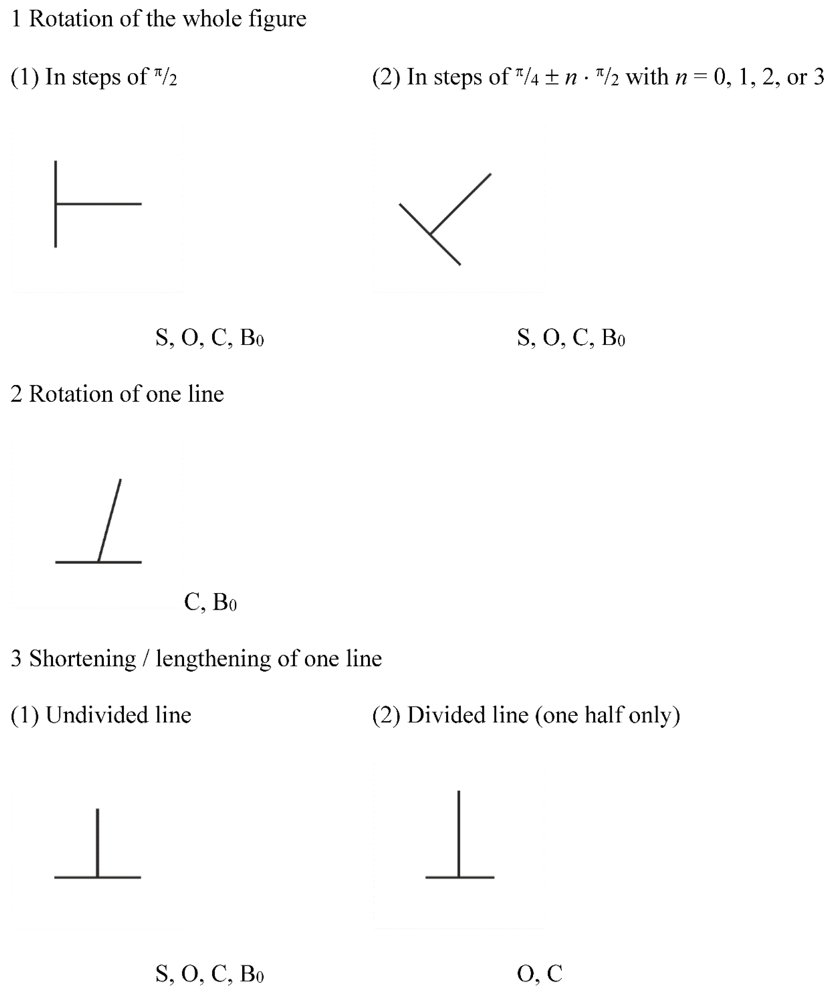
Proceeding analogously to the L, the T figure can also be rotated in its entirety, or its constitutive lines can be tilted relative to one another. The first measure leaves all the geometrical properties of the figure intact, but, at oblique orientations of the figure, it removes the horizontal-vertical component of the illusion, separating the factor of bisection [50,51]. The second move only retains connectivity and bisection, and it significantly reduced or even inverted the illusion, depending on the overall orientation of the figure and the use of a particular psychophysical method (the method of adjustment [47]. With the method of constant stimuli, an additional dissection of the T (case 4–2(1)) led to a further attenuation of the illusion for an inverted, upright T (i.e., a ⊥) with its undivided line tilted, and again to a reversal of the illusion for a laterally oriented T with its divided line tilted [52]. Different from the L, shortening the undivided line of the T preserves all its geometrical characteristics, but easily eliminates the illusion, whereas changing the length of the divided line in either direction only retains orthogonality and connectivity. Translating one line of the T vertically off the other line keeps symmetry, orthogonality and, implicitly, bisection, but attenuates the illusion [53]. Translating one line of the T along the other line keeps orthogonality, but also attenuates the illusion [54]. Translating one line of the T in an oblique direction, isolates orthogonality. Finally, adding rotations to these three cases implicitly keeps bisection in the first case and connectivity in the second case, but, in the third case, a rotation removes all geometrical singularities, and similar to the dissected, tilted-lines Ls, should null all illusion–although a horizontal-vertical bias still has to be controlled for.

3. The Cure of Sighting

Kundt [15], discussing the Poggendorff illusion, emphasized that it was important, “dass man ohne lange zu urtheilen und zu visiren, senkrecht auf die Zeichnung sehen muss” [to look orthogonally at the drawing without extended judging and sighting] (p. 118). Kennedy and Portal [27] let naïve observers exactly do this with the result that the Poggendorff, the Ebbinghaus, and the Hering illusions (plus some others not considered here) vanished when inspected from specific vantage points and a glancing angle of 15°. For the Poggendorff figure, the illusion was dispelled with sighting along the diagonal, objectively collinear lines. For the Ebbinghaus configuration, the effective vantage point was to one side of the figure–namely, looking at it along an imaginary line that connects the midpoints of the two inner circles, with the circle surrounded by larger ones near and the other one far. For the Hering display, the illusion vanished when observers looked along an imaginary line between the parallels (In Kennedy and Portal’s [27] version of the Hering illusion, this line was actually present (although not precisely centered between the target parallels), but the convergence point had been replaced by a white circle. The symmetry groups of the parts of the Ebbinghaus figure used were c5 for the large-annulus part and d8 for the small one).

In Kennedy and Portal’s [27] study, the angle at which to inspect the illusion figures was fixed. Would observers be able to find a glancing angle at which illusions were eradicated when presented at different slants? To answer this question, I set up a simple, computerized experiment. Only four illusion figures were used: the T, a ten-dots version of the Oppel–Kundt figure, the Müller–Lyer figure, and, again, the Ebbinghaus circles. The Poggendorff and Hering figures were not used because Kennedy and Portal’s findings seemed sufficiently clear, and the Zöllner figure was discarded because of its complexity, and also its similarity to the Hering figure (The fact that the Zöllner illusion vanishes when the observer is looking along the parallel lines at an angle, had been noticed already by Hofmann [3] (p. 117), who, in turn, credited Hering [26] for this observation. Looking orthogonally at the parallel lines would enhance the illusion–contrary to what Zöllner [21] had claimed). The L was not used because, if its d1 axis of mirror symmetry is oriented vertically (as was mandatory for the experiment), the illusion vanishes (cf. my Figure 2–1 in Section 2, and the data reported in [43] (p.379)). Eventually, the Ponzo figure was not used because, in my view, it contains an irremovable confound (In the original Ponzo figure, the circle (or line) that is closer to the vertex will always be nearer to the converging lines, when the two inserted items (which are to be compared) are similar in size. Recently, I constructed a deconfounded version of the illusion figure by adding a mirror-symmetric second pair of converging lines and inserting single lines into each V-figure [55]). By using the scroll wheel of a conventional computer mouse, observers were asked to virtually slant pictorial illustrations of the illusion figures around a horizontal axis backwards or forwards until the two critical elements of the figures which had to be compared appeared to be congruent. The hypothesis was that observers would slant that half of a picture away from them which contained the larger appearing item.

3.1. Method

3.1.1. Participants

Ten psychology undergraduates took part in the experiment. The number of participants had been decided upon a priori in order to achieve statistical power of 1 − β ≥ 0.95 for a repeated-measures analysis of variance (rmANOVA) with α = β = 0.05, and f ≥ 1 [56]. Written, informed consent was obtained from all participants, and they were treated in accordance with the Declaration of Helsinki [57]. All participants had normal or corrected-to-normal vision, and all served in partial fulfillment of a class requirement. The Department’s Ethics committee had declared the experiment exempt.

3.1.2. Apparatus

The apparatus consisted of a computer screen (size: 59.6 × 33.5 cm; resolution: 2560 × 1440 pixels; response time: 3 ms), which was used for stimulus presentation, and a conventional computer keyboard and mouse, the space bar and scrolling wheel of which, respectively, were used to deliver responses. Scrolls had a resolution of 0.5° and could go from +90° to −90°. The screen was oriented frontoparallel at a distance of 44 cm from the observer. Stimuli, drawn from thin black lines or small dots (width or diameter = 1.25 mm = 9 arc min visual angle), were presented within a fixed, rectangular, light grey window (width: 21 cm; height: 29.5 cm; plane visual angles: 26.8° and 37.1°, respectively; luminance: 228 cd m⁻²; CIE-coordinates: x = 0.312; y = 0.332; Weber contrast between stimulus elements and background: C_W = −0.998); the rest of the screen was dark (0.355 cd m⁻²), and there was only faint, indirect illumination of the room.

In order to retain maximum comparability to Kennedy and Portal’s [27] study, viewing was binocular with no head restraint. As instructed and controlled by the experimenter, all observers kept a fairly stable head position. Since the stimulus was a cyclopean computer animation, different from Kennedy and Portal’s mechanical set-up, there was no binocular parallax, though.

3.1.3. Stimuli and Responses

As already mentioned in Section 3, four stimulus figures were used: the T, a ten-dots version of the Oppel–Kundt figure, the Müller–Lyer figure, and the Ebbinghaus circles. The T and the Müller–Lyer figure were shown at their canonical orientations with the T’s undivided line vertical and with the Müller–Lyer shaft lines horizontal. The Oppel–Kundt and the Ebbinghaus stimuli were rotated 90° so that the two parts of the figures were one above the other. All stimuli were shown at two orientations which were obtained by rotating the figures by a half-turn (see the insets in Figure 4). For the T, the Oppel–Kundt, and the Müller–Lyer figures, three variants were created with the two lines of the T, the two parts of the Oppel-Kundt, and the two shaft lines of the Müller–Lyer either identical in length (6.5, 7, or 7.5 cm = 8.4°, 9.1°, or 9.7° visual angle) or one line or extent 0.5 cm shorter or longer. Hence, for these stimuli, there were two orientations times nine length combinations, making for 18 different stimuli per figure, all of which stimuli were repeated once. For the Ebbinghaus figure, the diameters of all circles remained constant, and the stimulus was repeated eight times at each orientation, making for another 16 stimuli, which together with the other stimuli added up to 124 trials per participant. The reasons for treating the Ebbinghaus differently were comparability with Kennedy and Portal’s [27] conditions and the incommensurability of the length variation applied to the other figures with the overall size of the stimulus.

Prior to the experiment, the experimenter demonstrated to each participant how the computer animation to be shown had been produced. She held a DIN A 4 upright cardboard (21 × 29.7 cm width to height), on which the Hering illusion figure had been printed, with her hands at the ends of the cardboard’s unmarked midline and rotated it forwards and backwards while keeping the midline at eye-height. Then, the participant was encouraged to do the same her- or himself to see how the perspective view of the illusion figure changed with the direction and amount of slant of the cardboard.

For the experiment, stimuli, arranged in random order, were initially shown at frontoparallel orientation. Participants were instructed to use the scroll-wheel of the computer mouse to change the slant of the picture they saw: scrolling forwards would make the upper half of the picture recede into depth and scrolling backwards the lower half. When content with their setting, observers pressed the space bar of the computer keyboard, which automatically started the next trial after a delay of 200 ms. No time limit was set. Two participants completed the whole experiment within half an hour, whereas two others needed close to one and a half (the average was one hour). There were no systematic differences between fast and slow responders.

3.2. Results

The results can be read off Figure 4 at a glance. For the T, the Müller–Lyer figure, and the Ebbinghaus circles, the hypothesis was corroborated: When the longer appearing line or circle was in the upper half of the stimulus picture, the great majority of observers scrolled this half away from them, and in the opposite case, towards them. Mean results for the Oppel–Kundt stimulus were exactly opposite to the hypothesis.

The angular settings were not perfectly symmetric, but roughly, they corresponded to amounts of illusion as typically reported for the illusions used. For example, for the T, which had been rotated around the midpoint of its undivided line, the average slant was 24.76°. At this inclination, the visual angle of the T’s undivided line, if 7 cm long, was 8.27° (≡6.4 cm), which is a reduction of 9.12 % as compared to the frontoparallel visual angle of 9.1°. Note, however, that during the backward slant of the upper half of the picture, the lower half underwent a forward slant, which increased the inverted T’s divided line by 0.28° (≡0.22 cm) or 3.1 %. Together, the adjusted optical minification of the T’s undivided line and the magnification of its divided line give a 12.22 % amount of illusion which is close to the best available estimate of 13.02 % for a vertically oriented T (or ⊥ [54]).

Statistically, the findings were confirmed by a Greenhouse–Geisser-corrected rmANOVA. There were no significant effects of the stimuli as such, only their orientation, F(2.332, 20.990)_Stimuli = 1.223, p < 0.319, η_p² = 0.120; F(1, 9)_Orientation = 14.993, p < 0.004, η_p² = 0.625, and also a significant interaction, F(2.920, 26.278) = 8.119, p < 0.001, η_p² = 0.474, which came about because of the deviating results for the Oppel–Kundt stimulus. Deviation contrasts showed that, for the Müller–Lyer figure, the effect was slightly greater than the overall mean effect, F(1, 9) = 5.544, p < 0.043, η_p² = 0.381, but simple and repeated contrasts showed that the effects for the T and for the Ebbinghaus figure did not differ in size from the one for the Müller-Lyer (both Fs < 1). Generally, there was a trend for the angular settings to correspond to the length calibration of the linear extents. For five participants, this trend was quite pronounced, but for the other participants, responses were mixed or even indifferent (Figure 5 shows means of all observers). In contradistinction to Figure 4, which refers to observers’ accuracy (i.e., observers’ ability to hit a predefined criterion), the data plotted in Figure 5 may be interpreted to reflect observers’ sensitivity (i.e., observers’ ability to discriminate between the calibration of the stimuli; see Section 4. for further discussion).

Statistically, there were no significant individual differences, F(1, 9) = 1.032, p < 0.336, η_p² = 0.103, but a detailed look at the data revealed that two observers responded to the Oppel–Kundt stimulus as predicted, two other observers responded to the T opposite to the prediction, and another two observers, respectively, responded to the Müller–Lyer or the Ebbinghaus stimuli contrary to the hypothesis.

3.3. Discussion

3.3.1. Do Illusions Really Go Away

In the abstract of their paper, and later in text, Kennedy and Portal [27] said that the illusions they had studied were “dispelled when the figures were viewed from glancing angles” (pp. 37, 42). As remarked by a reviewer, this statement may not actually be true. At a glancing angle of 15°, observers reported the true states of affairs, but the illusion-inducing elements of the figures studied may still have been necessary for the effects to occur. For example, if the annuli in the Ebbinghaus figure were removed, the two remaining circles might not appear equal when inspected at a slant. For my own experiment, I had been at pains to stress that observers’ task was to scroll pictorial representations of illusion figures to a slant at which the to-be-compared items would appear congruent. As I exemplified in Section 3.2, angular settings were expected to, and did, correspond to typical amounts of illusion. Hence, my procedure might be considered an alternative means to measure amounts of illusion.

Matters may be different for different illusions, though. As will be explained in more detail in Section 3.3.2, for some illusion figures–notably those, for which the task is to identify certain geometrical properties (e.g., the Poggendorff and the Hering illusions)–looking at these figures from a specific vantage point at a shallow angle provides a view of the true states of affairs as defined in terms of physical geometry. For some other illusion figures (e.g., those that I used in my experiment), even after a slant had been found at which the to-be-compared extents or sizes appeared equal, it still remained uncertain whether or not they really were in terms of physical geometry.

3.3.2. The Technique of Sighting and Seeing Things in Perspective

As an explanation, why looking at illusion figures from specific vantage points and at a shallow angle would dispel all illusion, Kennedy and Portal [27] offered the concept of “optical separation of the target elements”, suggesting that “smaller separation should improve comparisons” (p. 51). However, at a shallow glancing angle, not only do stimulus elements move closer together, they also undergo perspective contortion. This is most easily appreciated for the Müller–Lyer figure. Seen at a slant along the d1 axis of mirror symmetry, the shaft line which is farther away projects at a smaller visual angle so that the four endpoints of the shaft lines make for a perspective convergence gradient. At the same time, the space between the lines is also compressed, making for a foreshortening gradient [58]. Before attempting to explain Kennedy and Portal’s [27] as well as my newly secured findings in these terms, let us first be clear about the details of sighting.

The technique of sighting is known since ancient times [59] and seems to have been used by the stone-age megalithic architects already [60]. It comes in two forms: Either you look at two items (e.g., the top-ends of two stakes) at eye-height, or you look along a straightedge of variable inclination towards a distant goal. In this latter manner, sighting has been used to determine the distance of a ship approaching the shore–by transferring the angle of inclination to a position along the shore where the target distance could be measured [61]. Applied to illusion figures as done by Kennedy and Portal [27], it is only for the Poggendorff figure that sighting proper applies, because here observers have to decide on the collinearity of the two diagonals. In fact, except for putting a sufficiently long straightedge side-by-side the diagonals, it is difficult to see by which other means than sighting the task could be solved at all. For the other figures, it was true that observers looked at them from a specific vantage point at a shallow glancing angle, but they did not sight along a straightedge, and no use was made of the glancing angle. Hence, the explanation for the effectiveness of the vantage point and / or the glancing angle must be sought elsewhere.

In the cases of the Hering and the Zöllner figures, the task is to decide on the parallelism (or equidistance) of two or more lines. Glancing at these figures along the objectively parallel lines at a shallow angle turns the texture of the converging or tilted lines so dense that their orientations are no longer clearly discriminable; hence, the effects they exert at orthogonal viewing conditions seem to diminish. This hypothesis can further be tested by drawing the converging and tilted lines at low contrast. Note that, considered as sighting along one’s direction of gaze, sighting seems to allow for some tolerance. Remember from Section 3.1.2. that Kennedy and Portal’s [27] subjects “inspected the figures binocularly in free viewing (i.e., with no head restraint)” (p. 41), yet the apparently curved parallels of the Hering figure straightened out. However, why does sighting or glancing at an angle dispel the other illusions?

Looking at the Ebbinghaus or the Müller–Lyer figures at an angle along the d1 axis of mirror symmetry corresponds to looking–outdoors–at identical objects as these recede into the distance. The apparent diminution of sizes constitutes a minimum, two items, optical texture gradient [40]. For the Ponzo illusion, a figure with more than two parallel lines has been constructed [62], making for a more impressive gradient [4](p. 35: Figure 2.34). On the assumption that observers are adapted to the trigonometric functions that govern these gradients, observers may judge the diameters of the central circles in the Ebbinghaus display and the parallel lines in the Müller–Lyer figure according to the visual angles at which they project. Since these angles differ by a specific amount that is yoked to one’s glancing angle, it should be possible to find a glancing angle at which the visual angles apparently are the same so that the to-be-compared items appear to be congruent–as happened in Kennedy and Portal’s [27] as well as in my experiment.

3.3.3. Utilizing Perspective Distortions to Find States of Apparent Congruence

How, then, did observers in my experiment succeed in adjusting the slant of the visual-illusion figures, so as to annihilate the illusions, and why were settings opposite to the prediction for the Oppel–Kundt stimulus? The suggestion here is that observers exploited perspective distortions (The word perspective is used here in a double sense: as an adjectival qualifier and as the name of a specific form of perspective distortion). With the stimuli used, such distortions come in three forms: perspective, foreshortening, and distortion of shape [58]. Perspective refers to the apparent shortening of horizontal extents as these recede into depth, foreshortening to the apparent shortening of vertical extents, and distortion of shape (which is actually a consequence of the first two effects) to the compression of shapes. Perspective is most easily apprehended with the Müller–Lyer stimulus, where the two parallel horizontal lines make for a minimum texture gradient [40], but it is also present in the T-figure. Distortions of shape are most obvious with the Ebbinghaus display, the circles of which deform into compressed ellipses. Foreshortening occurs with all stimuli, but due to the small size of the dots, it is nearly isolated in the Oppel–Kundt stimulus.

Observers responded in accordance with the hypothesis with the more complex stimuli in which at least two of the three features of perspective were present. For the way in which observers could slant the pictorial illustrations of the illusion figures, the crucial difference between perspective and foreshortening was that perspective yielded an increase in the visual angle of a horizontal extent when the picture was slanted towards the observer, whereas foreshortening yielded a decrease in both the visual angles of the two halves of the vertical extents, only to a different degree. This may have confused observers when dealing with the Oppel–Kundt stimulus, in which perspective and compression of an appreciable shape were absent.

Two more things may have contributed to the discordant finding for the Oppel–Kundt figure. In an earlier experiment [63], I found the Oppel–Kundt illusion to be significantly attenuated when the stimulus was oriented vertically instead of horizontally. The attenuation was even stronger for modified stimuli for which the two parts of the figure had been bent relative to one another to produce L-type figures. Then, the illusion was maximally reduced when the vertical part of the figure was empty and the horizontal part filled. These findings suggested that the Horizontal-vertical illusion (viz., the overestimation of vertical extents relative to horizontal ones [31]) only acted on the empty part of an Oppel–Kundt figure, balancing the effect of the filling. In my earlier experiments, stimuli were shown at different orientations. In the present experiment, observers saw vertically oriented Oppel–Kundt stimuli only. Hence, a stimulus range effect may have reinforced the illusion’s attenuation, leading to its reversal for many observers.

The reason why the other elements of the presently discussed illusion figures seem to have exerted less of an influence when these figures were inspected at a slant, may have to do with reduced or eliminated symmetry. The circles of the Ebbinghaus figure now all projected as compressed ellipses with approximate symmetry group d2 instead of d∞, and the arrowheads in the Müller–Lyer figure were no longer symmetric at all. Hence, these context features of the figures probably could not stabilize the illusory impressions, so that zero-illusion orientations of the figures could be found.

4. Observers’ Task Demands: Discrimination versus Identification

So far, I focused on the stimuli and the conditions of presentation and observation in research with geometrical visual illusions. Let us now consider the task demands. For illusion figures A to E in Figure 1, observers are usually asked to say which of the two linear extents shown is the greater or the smaller one. For the Ebbinghaus figure, the task is typically framed in terms of the sizes of the inner circles, but this is equivalent to a judgment of the circles’ diameters or radii. In all these figures, concerning the true state of affairs, there are three possibilities: one or the other of the extents may in fact be greater or smaller, or they may be the same. If there is no further variation, observers’ task is to classify stimuli into one of the three categories (If the experimental procedure is two alternative forced choice (2AFC), the same category is not provided, and observers, if uncertain, are requested to respond at chance. The reason to shun same responses is because they are indistinguishable with regard to correct identification of sameness versus chance performance due to uncertainty or insensitivity (but see [64] for arguments in favor of 3AFC)). If length is varied in more than three steps–or in a factorial design–observers’ task is to compare extents pairwise, and to discriminate them in ordinal terms.

For the Poggendorff figure, the task posed, in contradistinction, is one of identification, namely to state whether the two diagonals are aligned or not. Similarly, for the Hering and Zöllner figures, people are usually asked whether the nonoblique lines are parallel or not. Although, for the Poggendorff, degrees of alignment can be instantiated, and for the Hering and the Zöllner, the number and relative orientation of the obliques can be varied, the response format will necessarily remain dichotomous, with the number of types of stimuli and the number of response alternatives being the same and, with regard to correctness, being bijectively related [28].

Thus, the nine illusion figures shown in Figure 1 seem to fall into two classes, as they require different kinds of responses (Actually, for illusion figures A to F, the task can also be framed in terms of identification, if the instruction reads “Are the two linear extents congruent or not”). However, with illusion figures, identifying responses almost unavoidably intrude into discrimination tasks. As demonstrated in Figure 2 and Figure 3 in illusion research, observers are typically operating under uncertainty near threshold. Even if told that in no case the to-be-compared stimulus elements are identical, they may–and most often will–appear to be so. Such stimuli, then, will invite same responses even if these are not allowed.

When data from two-alternative forced-choice experiments are analyzed in terms of psychometric functions, two parameters of such functions (usually: cumulative Gaussians) can be determined–bias versus sensitivity–which are typically uncorrelated [65]. Bias refers to the displacement of the function’s 50% point relative to true zero, and sensitivity to the function’s slope or a conventionalized threshold measure (most often, half the difference between the 25% and 75% points of the function as projected onto the abscissa). Traditionally, researchers dealing with illusions have focused exclusively on bias, and only recently has it become more common to look at sensitivity as well (e.g., [66]) (Historically, this bias may have come about due to a preference for adjustment procedures. For the experiment reported in Section 3, it was easy to plot data with regard to observers’ accuracy (or amount of illusion; Figure 4), but it was less obvious how to demonstrate their sensitivity (Figure 5). In fact, the procedure used did not allow for a quantitative comparison of the two measures). The suggestion here is that the independence of bias and sensitivity comes about because observers get mixed up with competing task demands.

If an experiment, in which observers have to discriminate stimuli, contains trials with both very similar and very different stimuli, there will be two types of trials, one of which requires discrimination, whereas the other one invites identification. The trials with obviously different stimuli have to be responded to by discriminative ordinal judgments, but the trials with similar or identical stimuli are likely to trigger responses of the same-different dichotomy which qualify as identifications as defined above. With illusion figures, observers often fail with regard to the identifying responses–falling prey to illusions–but usually succeed with the discriminative ones.

5. Conclusions

Geometrical visual illusions mainly occur with regular, especially symmetric figures that are composed from the elements of Euclidean geometry and viewed under contrived conditions of presentation and observation. Several illusions can be overcome by decomposing the figures or by viewing them in perspective. Falling prey to an illusion does not preclude discriminative sensitivity. Of the two parameters of a psychometric function, the response bias is probably caused by an identifying response–deciding on the dichotomy of sameness versus difference–whereas the sensitivity (or difference threshold) is probably due to an assortment of the stimuli according to an ordinal metric.