Article

Automatic Identification and Intelligent Optimization of Tunnel-Free Curve Reconfiguration

1
School of Rail Transportation, Soochow University, Suzhou 215006, China
2
School of Transport and Civil Engineering, Nantong University, Nantong 226019, China
*
Author to whom correspondence should be addressed.
Symmetry 2022, 14(12), 2505; https://doi.org/10.3390/sym14122505
Submission received: 15 October 2022 / Revised: 17 November 2022 / Accepted: 21 November 2022 / Published: 27 November 2022
(This article belongs to the Section Engineering and Materials)

Abstract

:
Extracting complete cross-sectional geometric features from the large amount of point cloud data acquired by laser scanners plays an important part in the detection of deformations in tunnel inspection projects. Tunnel cross-sections have symmetrical geometric features, and information is traditionally collected manually. The traditional manual extraction of point clouds is inefficient and limited by the subjectivity of the operators when addressing the problems. This paper proposes a new algorithm for the automatic identification of tunnel lining section curves, the rapid separation of common interference targets, and the optimization of curve geometry features. The innovation of this approach lies in the combination of B-spline and Euclidean clustering methods and the comprehensive evaluation of the denoising results in terms of precision, recall, F-score, and rand index (RI). In this way, the automatically extracted health point cloud data are refitted to optimize the tunnel profile model.

1. Introduction

Tunnels are subject to varying degrees of disease during construction and operation. Cracks, water leakage, deformation, etc., pose serious challenges to the safety of the tunnel. If they are not detected and warned about in time, small defects can evolve into more serious ones, threatening the safety of trains and even causing incalculable safety accidents. Tunnel deformation is not sudden damage; it is slowly deformed over time during operation and cannot be observed visually compared to cracks and leaks. Therefore, it is necessary to monitor and detect tunnel deformation in real time. The traditional method relies on manual inspection, but fewer data points are collected and cannot reflect the complete tunnel deformation. In addition, the traditional method has a low collection accuracy, and the data collection process is easily affected by the operator’s subjectivity [1]. The efficiency of collecting a representation of the whole tunnel is low, and the real-time detection of tunnel deformation cannot be realized.
The application of visual perception technology to tunnel monitoring projects has great potential in tunnel inspection engineering [2]. Technologies such as laser scanning and photogrammetry can effectively achieve high-precision geometric modeling of tunnel profiles and provide reference information in the event of subsequent tunnel deformation, water leakage, cracking, or detection of falling blocks. In recent years, scholars have conducted in-depth research and proposed constructive solutions. The key step in these methods is to remove the interference from the original point cloud and extract the cross-section of the tunnel [3]. Farahani et al. developed a point cloud scaler to obtain a small-size geometric model of the tunnel by applying a displacement from the exterior wall and compensating for missing point clouds through additive manufacturing [4]. Xu et al. improved model accuracy by locally fitting cross-sectional points and constructed their model using the concept of “circular likelihood”, which reduced the invalid iterations and saved a lot of computational time [5]. Cao et al. segmented the point cloud into blocks by identifying the bolt and liner joint locations, then calibrated the model features of each block before matching and combining them into the final tunnel geometry model [6]. Duan et al. investigated a cylindrical fitting algorithm to identify tunnel lining geometric features for high-density cylindrical point cloud features [7]. Yi et al. extracted elements based on intensity images for hierarchical modeling to remove noise interference [8]. Cheng et al. developed several classification algorithms identifying different components [9]. Liu developed a harmonic map-based algorithm to reconstruct the tunnel model and detect tunnel health based on the depth map [10]. Wang et al. rotated the central axis of the tunnel to obtain the cross-sectional attitude and removed the point cloud noise using fractional calculus [11]. These methods suffer from the problem of excessive removal of effective point clouds or chunking to increase the complexity of the work while improving the model accuracy. The problem of improving the denoising efficiency while reducing the local accuracy of the curve. Therefore, a new method is needed to ensure the continuity of curve fitting, high local accuracy and simple work.
To guarantee the high accuracy of the curve, we have to improve in the curve fitting method. Not limited to the tunnel scene, the methods of building geometric models are diverse. The least squares method is the most commonly used method for constructing geometric models. Curve modeling changes are complex, and singular matrices may appear, so the least squares method cannot meet the requirements of high-precision modeling. It is therefore necessary to optimize the least squares method. Song et al. introduced the Levenberg Marquardt algorithm to manage the fitting of horizontal and vertical curve transitions [12]. Lopez-Rubio et al. fit a parabola based on the minimum absolute error [13]. Sa et al. fitted a buried-hole conic model based on a circular curve [14]. Li et al. fitted an irregular curve with a diagonalized differential equation [15]. Xu et al. proposed approximating the tunnel profile curve using B-spline estimation [16]. The more surface parameters there are, the better B-spline perform [17]. Overfitting or underfitting curves are adjusted by changing the number of control points and the spline order [18]. The Bayesian information criterion verifies that the high-precision B-spline construction model fits the laser tracker results particularly well [19]. Based on the root-mean-square and processing time evaluation indexes compared with other tunnel point cloud model construction methods, the B-spline curve has fewer errors and higher efficiency [20], which provides reliable information support to subsequent finite element analysis and crack detection work [21]. B-spline curves are flexible for any free-form surface construction and the choice of B-spline method for overall fitting reduces the complexity rather than section chunking. Based on this, the B-spline curve was selected to fit and optimize the tunnel profile in our approach.
To ensure the continuity of curve fitting, we have to improve in point cloud denoising. Perfect removal of the interfering point clouds will definitely remove the valid point clouds by mistake and make the curve intermittent in the subsequent fitting process. Different point cloud filtering methods inevitably remove the valid point clouds. The clustering algorithm divides the data into different families according to their characteristics, which are unknown beforehand. The goal of clustering should be to obtain minimum inter-clan similarity and maximum intra-clan similarity. Euclidean clustering is an essential and operationally efficient clustering method that uses Euclidean distance as an indicator for family delineation. There are three categories which are division, hierarchy, and density clustering. Lee et al. implemented divisional clustering of urban scene areas based on Euclidean distance [22]. Liu et al. identified a non-flat terrain grid based on Euclidean distance to achieve hierarchical clustering of multi-level overhang features [23]. Xu et al. investigated the intelligent recognition of obstacles by robots and achieved density clustering of multiple objects in complex scenes based on Euclidean distance [24]. Euclidean clustering is also helpful for the deep processing of data. Wang et al. improved the robustness of the model through secondary fine clustering based on Euclidean distance after coarse classification of road infrastructure [25]. The distance threshold is the most critical parameter in the operation of the algorithm. Choosing the distance threshold based on a priori knowledge can result in a significant error in the point cloud within the family. Wen et al. designed the threshold adaptive algorithm to satisfy the requirement for different threshold values for different objects in different environments [26]. Based on this, this paper uses the clustering method to remove the interference. The innovation in our approach is that the original point cloud data are not clustered directly. After obtaining the residual maps of the B-spline fitted points and the original points, Euclidean clustering is used to divide the residual point clouds and identifies the optimal distance threshold based on the clustering index.
Our paper proposes a new tunnel section geometry construction algorithm based on B-spline curve modeling and Euclidean clustering denoising. The advantages of this algorithm are that it does not consider compensation for missing point clouds, it reduces the complexity of the work by modeling in chunks, achieves fast denoising, optimizes the section geometry model, and is accurate and robust. In Section 2, the algorithm flow and principles are described in detail. In Section 3, the setting of parameters is discussed. In Section 4, the experimental results and algorithm superiority are showed. In Section 5, the conclusions of this study and further research are outlined.

2. Method

The difficulty in automatically identifying tunnel models and removing common interference targets lies in the intelligence required to locate interference targets. The free curve property of the B-spline clearly reflects the local abrupt change of the point cloud and the offsetting of the curve by the interfering point cloud, so the residual point cloud is generated between the fitted point cloud and the original point cloud, where the outlier is the location of the interfering target. This method relies on Euclidean clustering to quickly traverse each point cloud in a cluttered residual map and remove outlier points. We propose an algorithm using B-spline fitting to model curves, Euclidean clustering to remove interference point clouds, and quadratic fitting to optimize the curves.

2.1. Motivation

The workflow described in this paper is shown in Figure 1, which is divided into three main stages covering B-spline fitting to model curves, Euclidean clustering for denoising, and curve optimization.
The disordered point cloud data acquired by the laser scanner are input to the algorithm for the B-spline fitting stage, where the point cloud data are first sorted and projected onto the 2D profile, then the optimal parameters are set, and finally the fitted point cloud data are obtained at the end of this stage. The next stage involves the Euclidean clustering section. First, the residual map of the fitted point cloud and the original point cloud are generated, then the k-dimensional tree (KD-Tree) is applied to divide the region and obtain the set of nearest neighbor points. Next, the optimal Euclidean distance threshold is set, and finally, the set of point clouds that are smaller than the threshold is extracted to end this stage.
The output point cloud set is returned to the original point cloud position to obtain the denoised, healthy point cloud. This is compared with the manually labeled point cloud, and the denoising results are analyzed based on the clustering index. The denoised point clouds are fitted again to obtain the optimized curve model.

2.2. B-Spline Curve

B-spline curves are an important method for constructing geometric features of tunnel sections because of the high accuracy and local modifiability of the feature polygons they approximate. In Equation (1), C(u) is a mathematical expression of the B-spline curve representing a linear combination of the control point P i and the basis function N i , p u , where the number of control points is n + 1. In Equation (2), U is a node vector that represents the set of non-decreasing nodes u, where the number of nodes is m + 1 and it must satisfy m = n + p + 1. In Equation (3), N i , p u denotes the i-th B-spline basis function, where the function order is p. When p = 0, the basis function is the step function in Equation (4), which means that it takes 1 on the node interval   u i , u i + 1 and 0 in other cases.
C ( u ) = i = 0 n N i , p ( u ) P i , u [ 0 , 1 ]
U = 0 , , 0 , u p + 1 , , u m p 1 , 1 , , 1 , u 0 , 1
N i , p u = u u i u i + p u i N i , p 1 u + u i + p + 1 u u i + p + 1 u i + 1 N i + 1 , p 1 u    
N i , 0 u = 1 if   u i u < u i + 1 0   otherwise  
For a more detailed description of the mathematical representation of the B-spline curve, refer to the standard literature, such as [27,28,29].

2.3. KD-Tree

KD-Tree is a structure for partitioning the data space, and it divides the residual cloud into different regions to speed up the clustering algorithm when it queries the nearest neighbor points [30].

2.3.1. Create KD-Tree

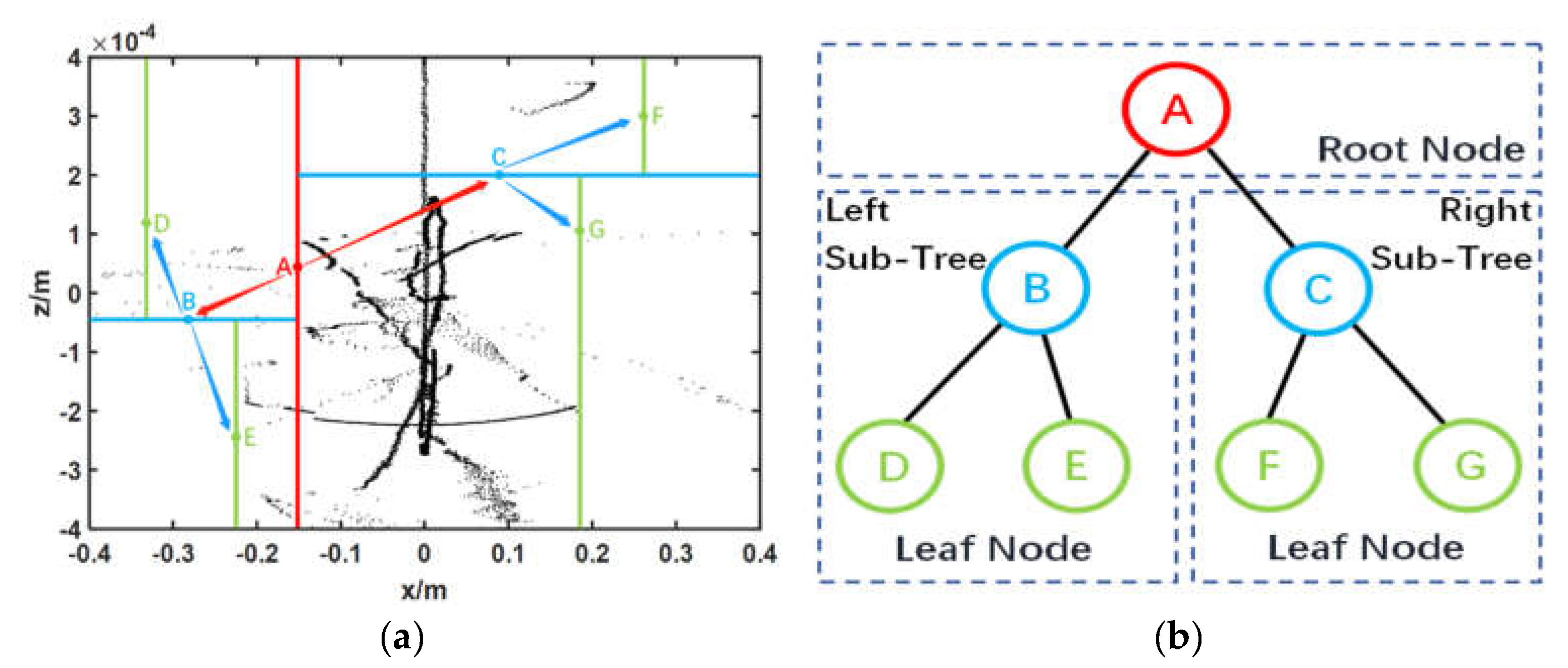
As shown in Figure 2a, the dimension with the largest variance in the residual cloud two-dimensional data set is selected, and then the median point A of this dimension is taken as the root node to divide the data set into left and right subtrees [31]. The above process is repeated, branching the left subtree to node B, then branching node B to nodes D and E. In the same way, the right subtree is branched to node C, and then node C is branched to nodes F and G. When it is no longer possible to divide it any further, it can be assumed that node DEFG is a leaf node, as shown in Figure 2b.

2.3.2. Nearest Neighbor Query

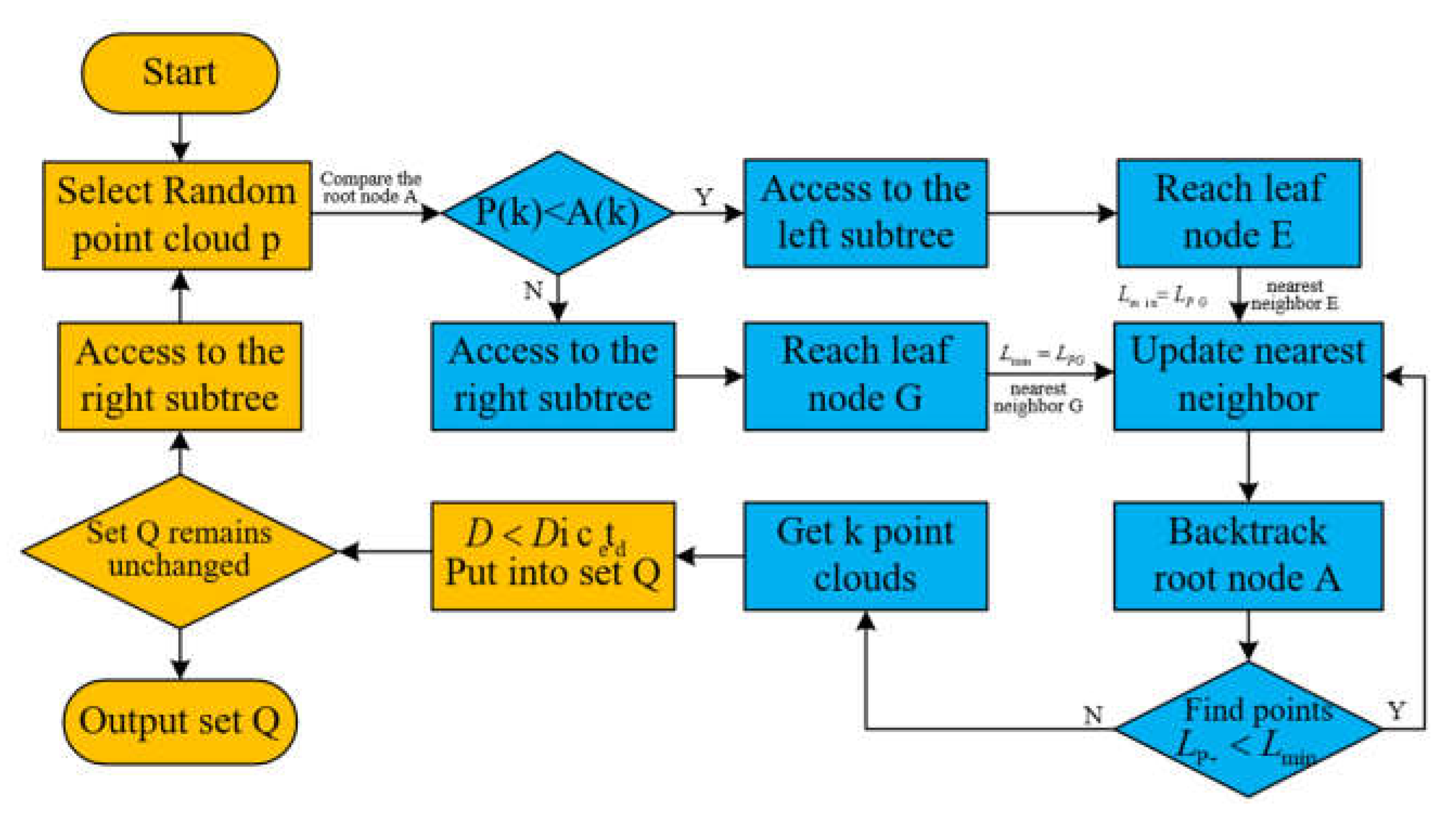
The query nearest neighbor process is shown in the blue dashed box in Figure 3. A randomly selected point cloud P is compared from the starting point A of KD-Tree all the way to the leaf node on the path, where P(k) represents the coordinates of P and A(k) represents the coordinates of A. If P(k) is smaller than A(k), the region to the left of the red line is visited. Otherwise, the region to the right of the red line is visited. In our example, we assume that G is the leaf node, and G is the nearest node of P. At this point, G is the nearest neighbor of P. The distance L between G and P is the minimum distance initially determined in the search path. The next step is to go back in the order of KD-Tree nodes from bottom to top to check if there are any other nearest neighbors. Then, a circle is drawn with distance L as the radius. In Figure 4a, there are no other nodes in the orange circle, then G is the final nearest neighbor point. In Figure 4b, the distance from point C to point P in the orange circle is smaller than L, and point C must therefore be included as a nearest neighbor. The whole nearest neighbor query process is completed when the search path is empty [32].

2.4. Euclidean Clustering

The residual point cloud data are simple to cluster, so the Euclidean clustering algorithm can be used to obtain faster operational efficiency. Equation (5) is the mathematical expression of Euclidean clustering. In our method, the point clouds with large residuals are automatically separated out by the clustering algorithm, and finally the removal of the tunnel contour interference is achieved.
Dict ed = x 1 x 2 2 + y 1 y 2 2

2.4.1. Clustering Flow

The residual maps of the B-spline fitted points and the original points are clustered objects. The interference points are discrete and small compared to the healthy point cloud, so the largest category in the residual map is the healthy point cloud set we want to obtain. The clustering process is shown in the orange box in Figure 3. The first search is completed by constructing a KD-Tree that traverses all point clouds and then quickly finds the k nearest neighbors to the random point cloud p. The specific process is described in Section 2.3 above. The second retrieval is completed by clustering points with inter cloud distance that is less than the Euclidean distance threshold   Dict ed into the set Q. To verify whether the set Q contains all the target point clouds, we continue to randomly select point clouds in the set Q, with the exception of point P, and repeat the above process. The whole clustering process is complete when the elements in the set Q do not change. In this way, we obtain the set of target point clouds and the points outside the set are the interference points. The elements in the set Q are the points in the residual map, so the points in the set Q are reduced to the original point cloud according to the position relationship in order to obtain a healthy point cloud set.

2.4.2. Evaluation Indicator

In our method, manually labeled point clouds with real labels are verified, and the effectiveness of Euclidean clustering is comprehensively evaluated based on four metrics: precision, recall, F-score, and RI. A confusion matrix is generated as shown in Table 1, where true positive (TP) denotes the number of healthy point clouds in set Q; false positive (FP) denotes the amount of noises in set Q; false negative (FN) denotes the number of health point clouds not in set Q; and true negative (TN) denotes the number of noises not in set Q.
The mathematical expressions of precision, recall, F-score, and RI are in Equations (6)–(10), where F β denotes the summed average and β denotes the weight. In this paper, β = 1 is chosen to indicate that accuracy and recall are equally important.
precision   = TP TP + FP
recall = TP TP + FN
RI   = TP + TN TP + FP + TN + FN
F β = 1 + β 2 precision recall ( precision   +   recall )
F 1 = 2 precision recall ( precision   +   recall   )
Precision is between the interval [0, 1], with larger values indicating that more healthy point clouds are correct in the true values; recall is between the interval [0, 1], with larger values indicating that more healthy point clouds are correct in the true values; and F1-score is between the interval [0, 1], combining precision and recall, with larger values indicating better clustering of healthy point clouds. The RI is between the interval [0, 1], and larger values indicate better overall clustering results. Comparing this with the F1-score, also allows the clustering of the interference point cloud to be considered, in order to better reflect fluctuations in the clustering results.

3. Data Analysis

3.1. Data Acquisition

The raw point cloud data in this experiment were obtained from the 14 profiles of the tunnel acquired by the laser scanner in the field, and the labeled point clouds are the corresponding healthy point clouds after manual denoising. Sorted into profiles 1–14, the number of raw point clouds as well as the number of labeled point clouds is shown in Table 2.

3.2. B-Spline Parameter Selection

The sensitivity of values of B-spline parameters n and strata p were studied based on the mean squared deviation. We found that the B-spline curves performed best in terms of accuracy, robustness, and rate for n = 3 and p = 10. The specific research process is described in [33]. Therefore, n = 3 and p = 10 was selected as the B-spline parameters for this entire process.

3.3. Clustering Parameters Selection

The Euclidean distance is the most important parameter in Euclidean clustering, and the choice of its threshold value is directly related to the clustering effect. In this study, the distance threshold was gradually increased in steps of 0.005 from 0.005 to 0.040, and the change in the clustering effect was observed by reference to the discounted graphs of the four external indicators expected to obtain the optimal distance threshold. As shown in Figure 5a, the precision of 12 sets of profiles gradually decreases as the distance threshold increases to approach 0.9, and the data in profiles 6 and 9 appear anomalous. The recall increases gradually as the distance threshold increases to 1, as shown in Figure 5b. Figure 5a,b illustrates that the increase of the distance threshold leads to more and more point clouds being clustered into the set Q. Although the accuracy decreases, there are increasingly more healthy point clouds that are consistent with the labeled point clouds, so the clustering results are increasingly consistent with the manual labeling results. When the distance threshold is too large, although the recall rate can reach 1 to completely cluster the healthy point clouds, it will cause the set Q to become over-clustered with too many noisy point clouds resulting in a reduced denoising effect. The optimal distance threshold must be identified so that the set Q has as many healthy point clouds and as few noisy point clouds as possible. To achieve this, we use the F1-score index, which considers both accuracy and recall, as shown in Figure 5c, and basically reaches a maximum value at a distance threshold of 0.02, decreasing slightly after a smooth period. To observe the moment of descent more accurately, we use the RI, which takes into account the effect of healthy point clouds and noise. The decline starts at 0.025, as seen in Figure 5d.
Therefore, considering the precision, recall, F1-score, and RI trends, it can be concluded that the best Euclidean distance threshold is 0.02. It is worth noting that excessive density of the point cloud has an impact on the selection of the Euclidean distance threshold. The point cloud density needs to be reduced by down sampling before input to the algorithm, and the optimal Euclidean distance threshold of 0.02 still remains applicable.

4. Results

There are three parts to the output of the whole algorithm, which are the fitting and denoising of the tunnel 2D profile, the evaluation of the indexes compared with the manual denoising results and the optimized tunnel fitting curve.

4.1. Fitting and Denoising Results

The tunnel profile resulting from the first B-spline fit and Euclidean clustering denoising is shown in Figure 6 and Figure 7. Green represents the interference point clouds that were removed, red represents the retained healthy point clouds, and blue represents the fitted profiles.
Figure 6 is divided into three parts. At the top are two laser scans of the real tunnel, below on the left are six sets of profiles with excellent fitting and denoising, and on the right are six sets of profiles with slight offsets. The orange circles in the figure indicate the interference factors, and the denoising process has successfully removed interference from the free point cloud, guardrail, cable line, and tube buckle.
Figure 7 presents two sets of poorly fitted profiles, corresponding to profile 6 and profile 9. It can be observed in the orange box that the missing point cloud in this area makes the B-spline curve tend to be straight instead of curved, which leads to the incorrect removal of the correct point cloud in the subsequent denoising process. In other locations, the fitting and denoising results are excellent. On the right, it can be observed that a large number of humanoid interference point clouds appear in this area, which makes the B-spline curve drop suddenly and the fitting result deviate severely from the elliptic curve, resulting in the erroneous retention of the humanoid interference point clouds instead of the erroneous removal of the retained point clouds on the right side of the tunnel in the denoising process.
The fitting and denoising results suggest that the fit is excellent and the denoising is ideal for the normal data collected by the laser scanner, and a healthy tunnel point cloud can be obtained for subsequent optimization of the tunnel profile. In cases where point cloud data are missing, the fitted curve will be interrupted or straightened, which has some impact on denoising. When there are large and dense uncommon disturbances, such as humanoid disturbances, the fit will fail, the denoising will be meaningless, and the subsequent curve optimization will be disturbed. However, there is a low probability of humanoid interference in laser scanner acquisition data in real-life situations, and the entire fitting and denoising process remains sufficiently accurate and robust.

4.2. Indicator Results

The 14 sets of point cloud data are clustered optimally with the best denoising results when the Euclidean distance threshold value is taken as 0.02. The precision, recall, F1-score, and RI are listed in Table 3.
To analyze the data characteristics more clearly, a line graph was created as shown in Figure 8. The purple line depicts the change of precision, the green line depicts the change of recall, the blue line depicts the change of F1-score, and the orange line depicts the change of RI.
By combining Table 3 and Figure 8, it can clearly be seen that there is a downward cusp at the transverse axis 6 and a sharp downward cusp at the transverse axis 9. Profile 9 clustering anomalies are highlights in Table 3, with precision only 0.6858, recall 0.9334, F1-score 0.7907, and RI only 0.6737. The poor clustering of profile 6 in Table 3 with precision 0.8182, recall 0.9627, F1-score 0.8846, and RI 0.8044. Excluding the anomalous data of profile 9, the precision of the other 13 sets of data reached 0.9271 overall, with recall 0.9867, F1-score 0.9555, and RI 0.9190. The clustering index results are consistent with the results of the figure in Section 4.1. The clustering index results show that if the F1-score is in the interval (0.9, 1) the automatic denoising by the algorithm closely matches the manual denoising. If it is in the interval (0.8, 0.9), some point cloud data may have been missed. When it is below 0.8 or when a metric is too weak, there will be large, dense unusual disturbances in the point cloud data.

4.3. Optimization Results

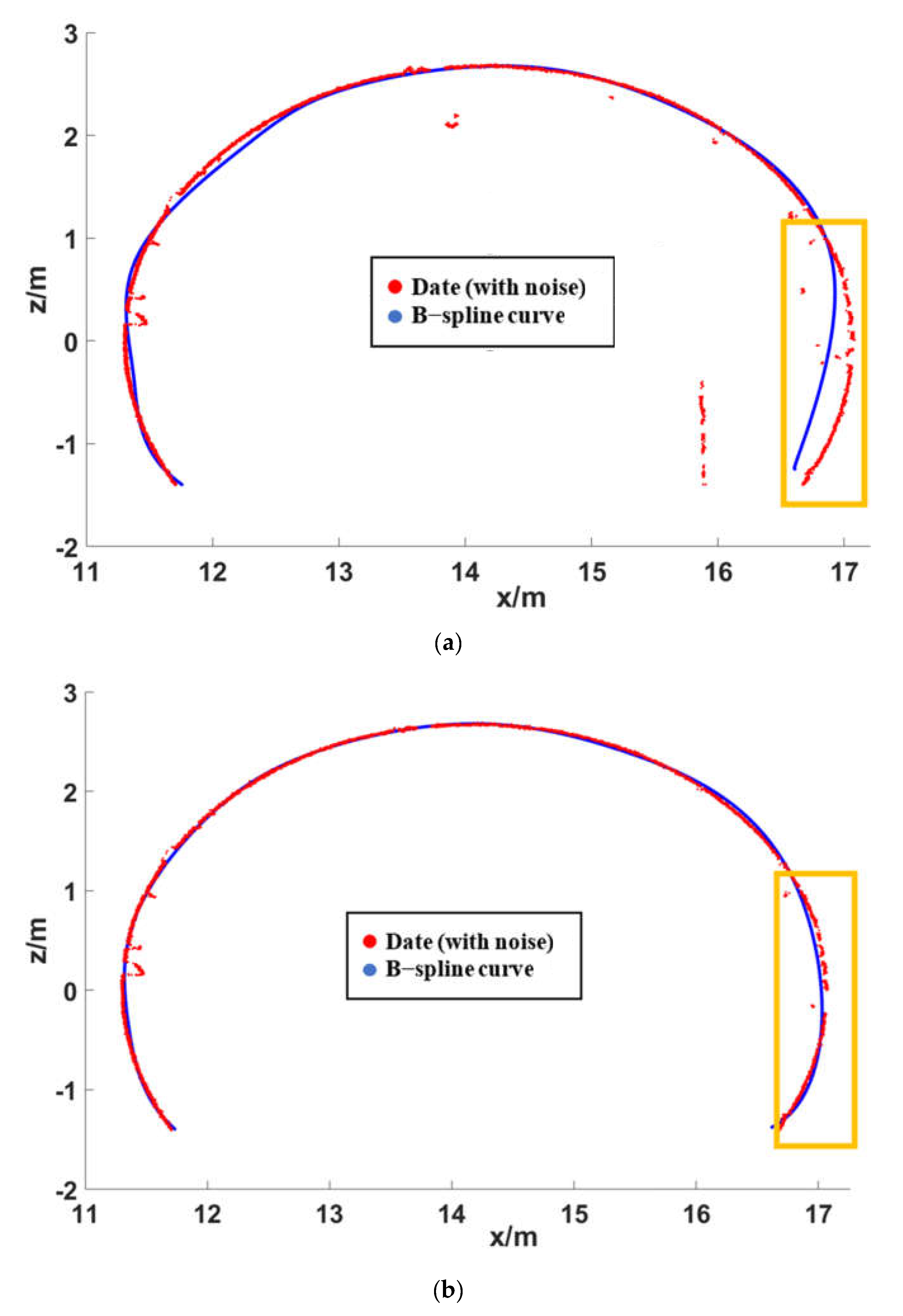
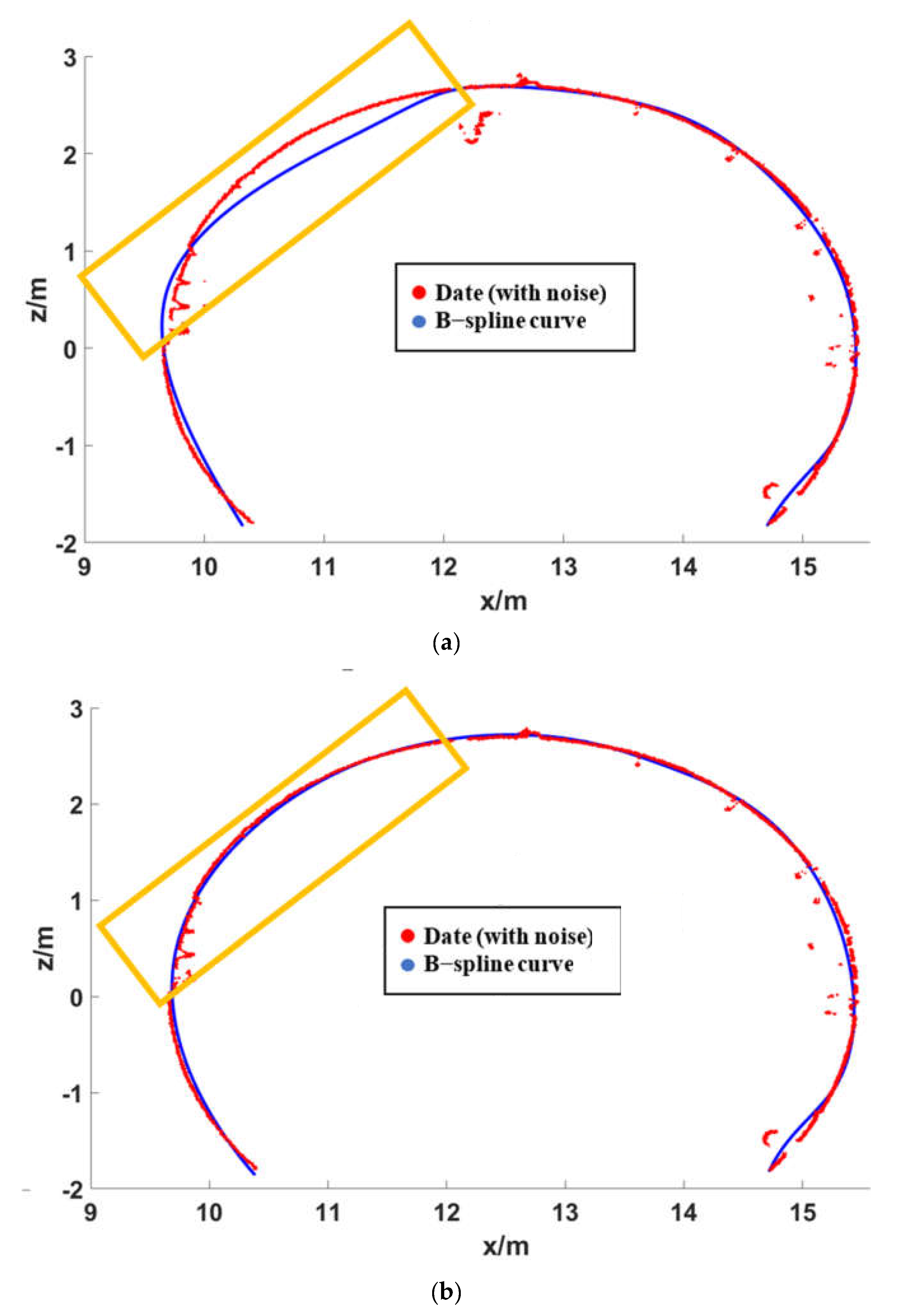
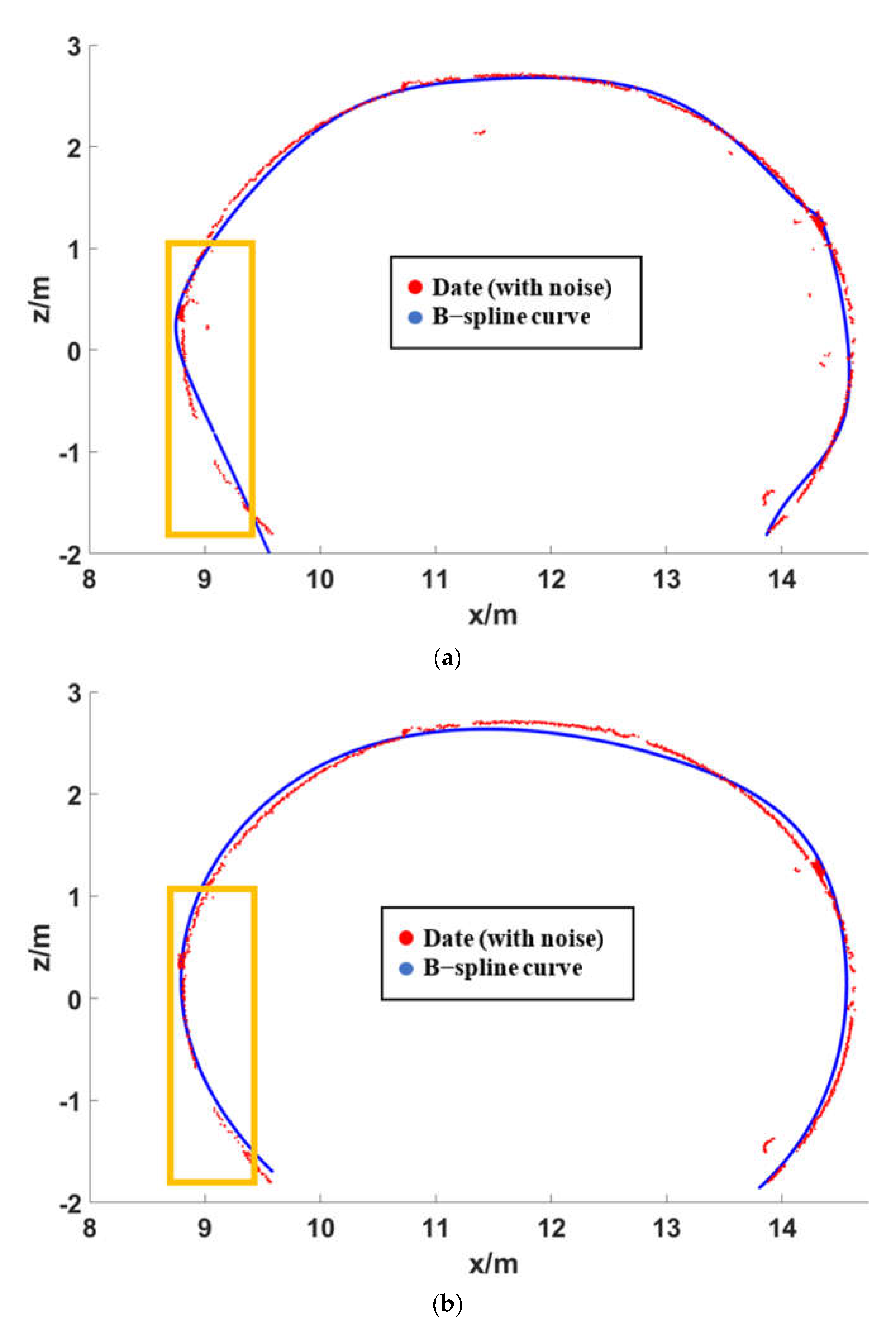
After obtaining the denoised healthy point cloud data and fitting the B-spline curve again, the curve geometry can be optimized to better fit the tunnel shape. As shown in Figure 9, Figure 10, Figure 11, Figure 12, Figure 13 and Figure 14, (a) is the first fitted profile and (b) is the second, optimized fitted profile, and the orange boxes highlight the differences between them. We can observe that Figure 9 is the typical profile of most cases of free point cloud interference, where the curve is slightly shifted inward, so that after removing the interference, the curve is closer to the actual tunnel shape. Figure 10 shows the interference from the tube buckle in the lower right corner, the depression is only present in a small section, and it disappears after the removing the interference. Figure 11 shows the interference from the guardrail, which has a more obvious leftward alignment on the right side of the curve. After removing the interference, the curve corrects to the tunnel shape. Figure 12 shows the interference from the cable line, which makes the curve deviate downward. After removing the interference, the curve returns to the original trend. Figure 13 shows the interference of the missing point cloud; the optimized curve fits the tunnel point cloud but is still offset. Figure 14 shows the humanoid interference, which is a large, dense uncommon interference, and the B-spline fitting curve leads to a subsequent residual clustering effect which is not satisfactory, so after the second fitting, the optimization curve is still not achieved.
The optimization results show that the B-spline fits the tunnel curve model nearly perfectly after removing the interference of common appendages. For large dense uncommon disturbances scanned by the laser scanner, such as humanoid disturbances, the denoising results are poor and the optimized curve still does not correctly reflect the true tunnel curve.

5. Conclusions

With the frequent occurrence of geological hazards, tunnel safety is receiving increasing attention. The rapidly increasing demand for inspection has driven innovation and the development of intelligent inspection techniques for tunnel structures. In this paper, we studied the construction, denoising, and optimization of the tunnel section model. Our contributions are as follows:
(i)
An automated algorithm based on B-spline curve and Euclidean clustering was constructed to identify, denoise, and optimize the tunnel point cloud model.
(ii)
KD-Tree accelerates the clustering of tunnel point clouds and improves the denoising efficiency.
(iii)
The influence of the Euclidean distance threshold on point cloud denoising was evaluated comprehensively using four indexes: precision, recall, F1-score, and RI, and the optimal Euclidean distance threshold for tunnel residual point clouds was determined.
(iv)
The effects of common and uncommon disturbances on the B-spline curve trend were observed by analyzing the curve-fitted profiles.
(v)
A comparison of algorithmic denoising results with manual denoising results from both qualitative and quantitative dimensions through analysis of the denoised profiles.
(vi)
A comparison of the results of the two B-spline fits, demonstrating that the optimized tunneling curve is highly accurate and robust.
In the next stage of our work, we will continue to improve the algorithm’s adaptability to address the impact of uncommon disturbances on the robustness of the tunnel profile construction and to extend it to other tunnel profile environments, such as rectangular tunnel models. In addition, we will rely on the tunnel profile model to complete the subsequent analysis of deformation.

Author Contributions

Methodology, X.X. (Xiangyang Xu), Z.W. and H.Y.; formal analysis, Z.W. and H.Y.; investigation, Z.W. and X.X. (Xiangyang Xu); resources, P.S., X.X. (Xunqian Xu), Z.W. and H.Y.; data curation, P.S., Z.W. and H.Y.; writing—original draft preparation, Z.W., F.X. and X.X. (Xunqian Xu); writing—review and editing, Z.W. and X.X. (Xiangyang Xu); project administration, P.S., X.X. (Xunqian Xu) and X.X. (Xiangyang Xu); funding acquisition, P.S., X.X. (Xiangyang Xu) and H.Y. All authors have read and agreed to the published version of the manuscript.

Funding

This research was funded by Natural Science Foundation of Jiangsu Province, China (No. BK20220502), Suzhou Innovation and Entrepreneurship Leading Talent Plan (No. ZXL2022488), Natural Science Foundation of Nantong, China (No. MS22020026) and National Natural Science Foundation of China (No. U1934209).

Institutional Review Board Statement

Not applicable.

Informed Consent Statement

Not applicable.

Data Availability Statement

The data presented in this study are available on request from the corresponding author.

Conflicts of Interest

The authors declare no conflict of interest.

References

  1. Wroblewski, A.; Wodecki, J.; Trybala, P.; Zimroz, R. A Method for Large Underground Structures Geometry Evaluation Based on Multivariate Parameterization and Multidimensional Analysis of Point Cloud Data. Energies 2022, 15, 6302. [Google Scholar] [CrossRef]
  2. Yasuda, N.; Cui, Y. Deformation estimation of a circular tunnel from a point cloud using elliptic Fourier analysis. Tunn. Undergr. Space Technol. 2022, 125, 104523. [Google Scholar] [CrossRef]
  3. Sun, W.X.; Wang, J.; Jin, F.X.; Li, Y.Y.; Yang, Y.K. An adaptive cross-section extraction algorithm for deformation analysis. Tunn. Undergr. Space Technol. 2022, 121, 104332. [Google Scholar] [CrossRef]
  4. Farahani, B.V.; Barros, F.; Sousa, P.J.; Cacciari, P.P.; Tavares, P.J.; Futai, M.M.; Moreira, P. A coupled 3D laser scanning and digital image correlation system for geometry acquisition and deformation monitoring of a railway tunnel. Tunn. Undergr. Space Technol. 2019, 91, 102995. [Google Scholar] [CrossRef]
  5. Xu, X.Y.; Yang, H.; Neumann, I. A feature extraction method for deformation analysis of large-scale composite structures based on TLS measurement. Compos. Struct. 2018, 184, 591–596. [Google Scholar] [CrossRef]
  6. Cao, Z.; Chen, D.; Peethambaran, J.J.; Zhang, Z.X.; Xia, S.B.; Zhang, L.Q. Tunnel Reconstruction With Block Level Precision by Combining Data-Driven Segmentation and Model-Driven Assembly. IEEE Trans. Geosci. Remote Sens. 2021, 59, 8853–8872. [Google Scholar] [CrossRef]
  7. Duan, D.Y.; Qiu, W.G.; Cheng, Y.J.; Zheng, Y.C.; Lu, F. Reconstruction of shield tunnel lining using point cloud. Autom. Constr. 2021, 130, 103860. [Google Scholar] [CrossRef]
  8. Yi, C.; Lu, D.N.; Xie, Q.; Liu, S.Y.; Li, H.; Wei, M.Q.; Wang, J. Hierarchical tunnel modeling from 3D raw LiDAR point cloud. Comput.-Aided Des. 2019, 114, 143–154. [Google Scholar] [CrossRef]
  9. Cheng, Y.J.; Qiu, W.G.; Duan, D.Y. Automatic creation of as-is building information model from single-track railway tunnel point clouds. Autom. Constr. 2019, 106, 102911. [Google Scholar] [CrossRef]
  10. Liu, M.H.; Sun, X.B.; Wang, Y.; Shao, Y.; You, Y.C. Deformation Measurement of Highway Bridge Head Based on Mobile TLS Data. IEEE Access 2020, 8, 85605–85615. [Google Scholar] [CrossRef]
  11. Wang, W.X.; Chen, W.W.; Kevin, W.; Shuang, L. Extraction of tunnel center line and cross-sections on fractional calculus, 3D invariant moments and best-fit ellipse. Opt. Laser Technol. 2020, 128, 106220. [Google Scholar] [CrossRef]
  12. Song, Z.F.; Yang, F.; Schonfeld, P.; Li, J.; Pu, H. Heuristic Strategies of Modified Levenberg-Marquardt Algorithm for Fitting Transition Curves. J. Surv. Eng. 2020, 146, 04020001. [Google Scholar] [CrossRef]
  13. Lopez-Rubio, E.; Thurnhofer-Hemsi, K.; Blazquez-Parra, E.B.; de Cozar-Macias, S.D.; Ladron-de-Guevara-Munoz, M.C. A fast robust geometric fitting method for parabolic curves. Pattern Recognit. 2018, 84, 301–316. [Google Scholar] [CrossRef]
  14. Sa, J.M.; Gu, H.W.; An, Y.L.; Luo, Y.J.; Zhang, Z.S.Y. Study on Curved Surface Fitting of Countersink Based on Point Cloud. IEEE Access 2020, 8, 106464–106470. [Google Scholar] [CrossRef]
  15. Li, X.J.; Chen, Z.Y.; Chen, J.Q.; Zhu, H.H. Automatic characterization of rock mass discontinuities using 3D point clouds. Eng. Geol. 2019, 259, 105131. [Google Scholar] [CrossRef]
  16. Xu, X.Y.; Kargoll, B.; Bureick, J.; Yang, H.; Alkhatib, H.; Neumann, I. TLS-based profile model analysis of major composite structures with robust B-spline method. Compos. Struct. 2018, 184, 814–820. [Google Scholar] [CrossRef]
  17. Zhao, X.; Kargoll, B.; Omidalizarandi, M.; Xu, X.Y.; Alkhatib, H. Model Selection for Parametric Surfaces Approximating 3D Point Clouds for Deformation Analysis. Remote Sens. 2018, 10, 634. [Google Scholar] [CrossRef] [Green Version]
  18. Yang, H.; Xu, X.Y.; Kargoll, B.; Neumann, I. An automatic and intelligent optimal surface modeling method for composite tunnel structures. Compos. Struct. 2019, 208, 702–710. [Google Scholar] [CrossRef]
  19. Yang, H.; Xu, X.Y. Multi-sensor technology for B-spline modelling and deformation analysis of composite structures. Compos. Struct. 2019, 224, 111000. [Google Scholar] [CrossRef]
  20. Xu, X.Y.; Yang, H. Robust model reconstruction for intelligent health monitoring of tunnel structures. Int. J. Adv. Robot. Syst. 2020, 17, 1729881420910836. [Google Scholar] [CrossRef]
  21. Xu, W.; Xu, X.Y.; Yang, H.; Neumanna, I. Optimized finite element analysis model based on terrestrial laser scanning data. Compos. Struct. 2019, 207, 62–71. [Google Scholar] [CrossRef]
  22. Lee, H.; Jung, J. Clustering-Based Plane Segmentation Neural Network for Urban Scene Modeling. Sensors 2021, 21, 8382. [Google Scholar] [CrossRef] [PubMed]
  23. Liu, H.Y.; Song, R.; Zhang, X.B.; Liu, H. Point cloud segmentation based on Euclidean clustering and multi-plane extraction in rugged field. Meas. Sci. Technol. 2021, 32, 095106. [Google Scholar] [CrossRef]
  24. Xu, X.B.; Zhang, L.; Yang, J.; Cao, C.F.; Tan, Z.Y.; Luo, M.Z. Object Detection Based on Fusion of Sparse Point Cloud and Image Information. IEEE Trans. Instrum. Meas. 2021, 70, 2512412. [Google Scholar] [CrossRef]
  25. Wang, D.; Wang, J.; Scaioni, M.; Si, Q. Coarse-to-Fine Classification of Road Infrastructure Elements from Mobile Point Clouds Using Symmetric Ensemble Point Network and Euclidean Cluster Extraction. Sensors 2020, 20, 225. [Google Scholar] [CrossRef] [Green Version]
  26. Wen, L.; He, L.; Gao, Z.H. Research on 3D Point Cloud De-Distortion Algorithm and Its Application on Euclidean Clustering. IEEE Access 2019, 7, 86041–86053. [Google Scholar] [CrossRef]
  27. Piegl, L.; Tiller, W. The NURBS Book; Springer: Berlin/Heidelberg, Germany, 1997. [Google Scholar]
  28. Farin, G. Curves and Surfaces for CAGD: A Practical Guide; Morgan Kaufmann: Burlington, MA, USA, 2002. [Google Scholar]
  29. Bureick, J.N.H.; Harmening, C.; Neumann, I. Curve and Surface Approximation of 3D Point clouds. Allg. Vermess.-Nachrichten. 2016, 123, 135–227. [Google Scholar]
  30. Liu, W.P.; Sun, J.; Li, W.Y.; Hu, T.; Wang, P. Deep Learning on Point Clouds and Its Application: A Survey. Sensors 2019, 19, 4188. [Google Scholar] [CrossRef] [Green Version]
  31. Cheng, D.Y.; Zhao, D.J.; Zhang, J.C.; Wei, C.S.; Tian, D. PCA-Based Denoising Algorithm for Outdoor Lidar Point Cloud Data. Sensors 2021, 21, 3703. [Google Scholar] [CrossRef]
  32. Lee, J.M. Fast k-Nearest Neighbor Searching in Static Objects. Wirel. Pers. Commun. 2017, 93, 147–160. [Google Scholar] [CrossRef]
  33. Xu, X.Y.; Wang, Z.H.; Shi, P.X.; Liu, W.; Tang, Q.; Bao, X.H.; Chen, X.S.; Yang, H. Intelligent monitoring and residual analysis of tunnel point cloud data based on free-form approximation. Mech. Adv. Mater. Struct. 2022, 1–10. [Google Scholar] [CrossRef]
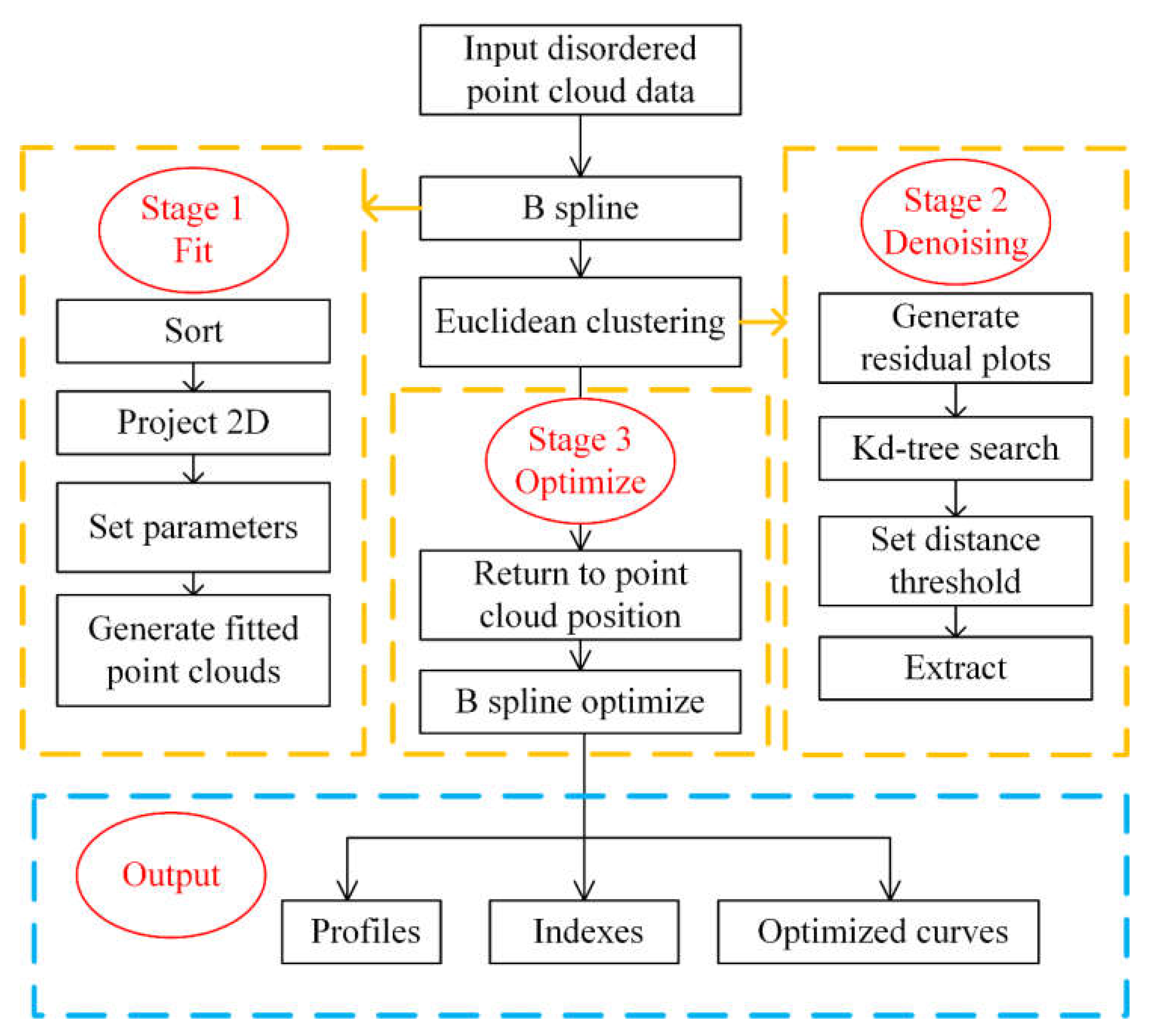
Figure 1. The workflow for this investigation.
Symmetry 14 02505 g001
Figure 2. Subtrees and nodes of KD-Tree: (a) in the residual graph; (b) in the tree diagram.
Symmetry 14 02505 g002
Figure 3. Euclidean clustering and KD-Tree workflow.
Symmetry 14 02505 g003
Figure 4. Nearest Neighbor Path Query: (a) no other node in the circle of radius PG; (b) other nodes in the circle of radius PG.
Symmetry 14 02505 g004
Figure 5. Clustering index of various distance thresholds. (a) Precision; (b) recall; (c) F1-score; (d) RI.
Symmetry 14 02505 g005aSymmetry 14 02505 g005b
Figure 6. Fitted profiles of excellence and slight offset.
Symmetry 14 02505 g006
Figure 7. Poor fitted profiles.
Symmetry 14 02505 g007
Figure 8. Index line graph of 14 groups of profiles.
Symmetry 14 02505 g008
Figure 9. Free point cloud interference and its optimization: (a) before optimization; (b) after optimization.
Symmetry 14 02505 g009
Figure 10. Tube buckle interference and its optimization: (a) before optimization; (b) after optimization.
Symmetry 14 02505 g010
Figure 11. Guardrail interference and its optimization: (a) before optimization; (b) after optimization.
Symmetry 14 02505 g011
Figure 12. Cable line interference and its optimization: (a) before optimization; (b) after optimization.
Symmetry 14 02505 g012
Figure 13. Missing interference and its optimization: (a) before optimization; (b) after optimization.
Symmetry 14 02505 g013
Figure 14. Humanoid point cloud interference and its optimization: (a) before optimization; (b) after optimization.
Symmetry 14 02505 g014
Table 1. Confusion Matrix.
Confusion MatrixPredicted Value
Set QNon Set Q
True ValueHealthy Point CloudTPFN
NoiseFPTN
Table 2. Number of raw point clouds and labeled point clouds.
ProfileRaw Point CloudsLabeled Point Clouds
11017897
21096943
31080935
411801100
513201232
616511286
719561808
823032134
940482673
1040673886
1165756078
1261665819
1375206581
1479886832
Table 3. Index data table of 14 sets of profiles.
ProfilePrecisionRecallF1-ScoreRI
10.95330.97770.96530.9381
20.90980.97350.94060.8922
30.88660.97860.93040.8731
40.94430.97090.95740.9195
50.95410.99590.97460.9519
60.81820.96270.88460.8044
70.95560.98730.97120.9458
80.94210.99860.96950.9418
90.68580.93340.79070.6737
100.98850.99770.99310.9867
110.94100.99130.96550.9344
120.97870.99380.98620.9737
130.88741.00000.94060.8890
140.89281.00000.94340.8973
Average0.92710.98670.95550.9190
The highlights represent anomalous data, bold represents poor data and others represent normal data.
Publisher’s Note: MDPI stays neutral with regard to jurisdictional claims in published maps and institutional affiliations.