
Heat and Mass Transfer Analysis of MHD Jeffrey Fluid over a Vertical Plate with CPC Fractional Derivative

 and
and 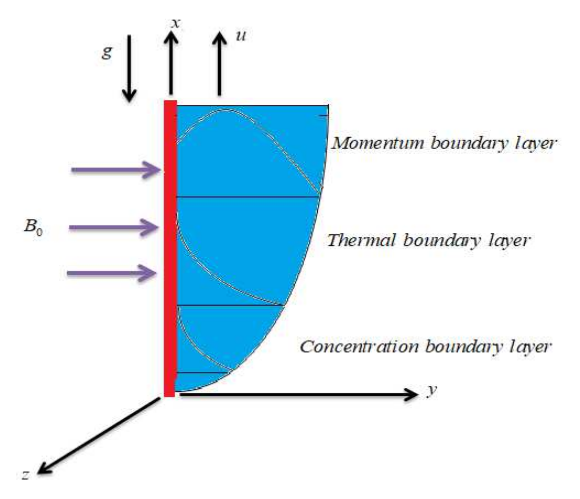
Abstract
1. Introduction
2. Problem Formulation
3. Ordinary Solution
3.1. Calculation of Temperature
3.2. Calculation of Concentration
3.3. Calculation of Velocity
4. Fractional Solution
4.1. Fractional Thermal Diffusion
4.2. Fractional Concentration
4.3. Fractional Velocity
5. Result and Discussion
6. Conclusions
- Increasing the values of , , Gr, and Gm increases the fluid’s velocity.
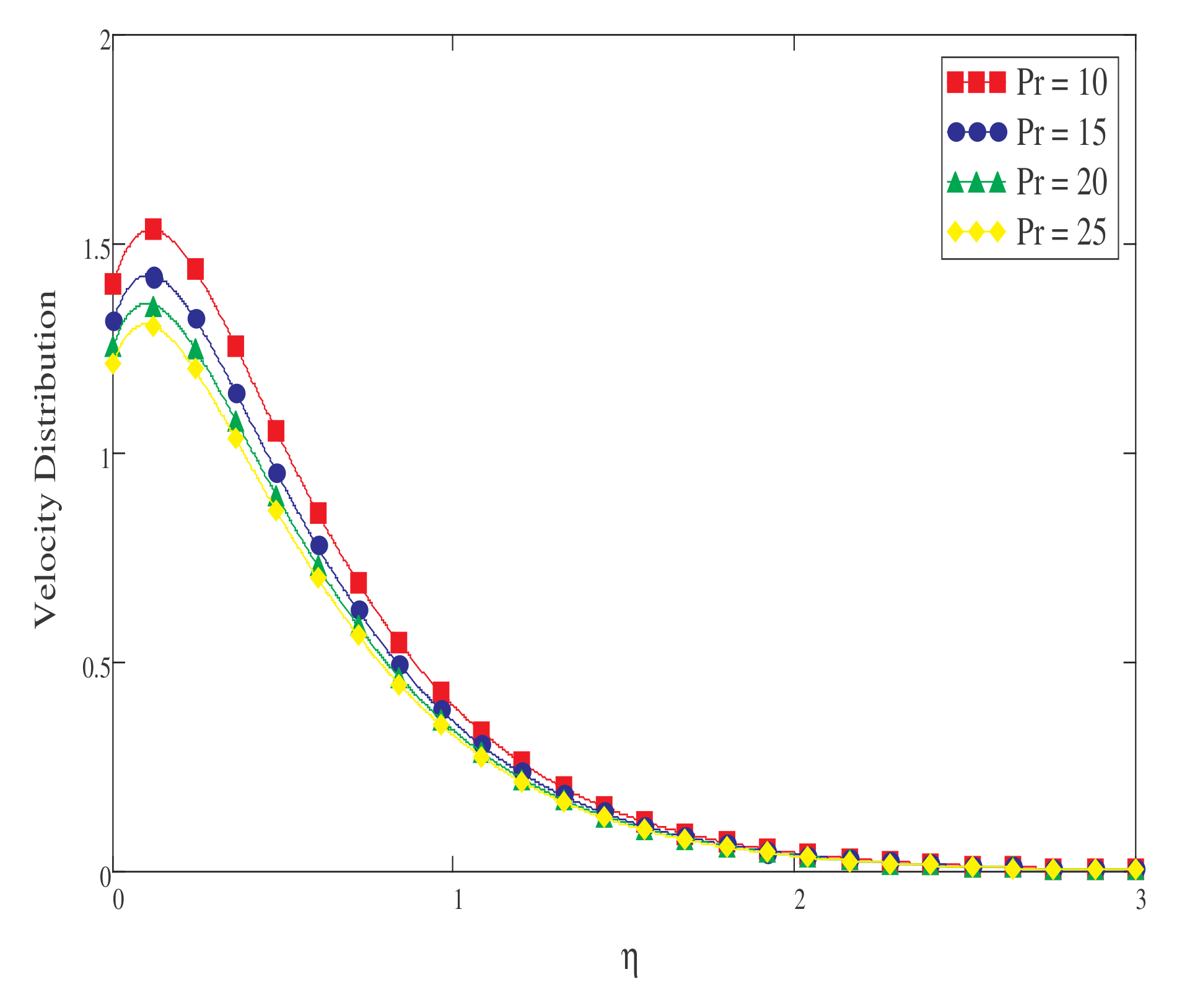
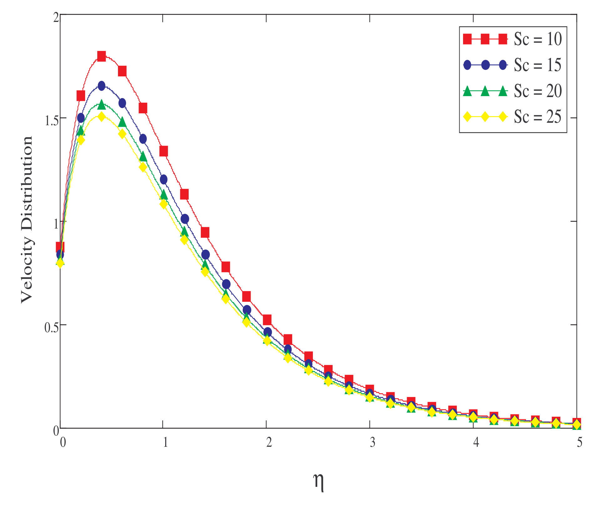
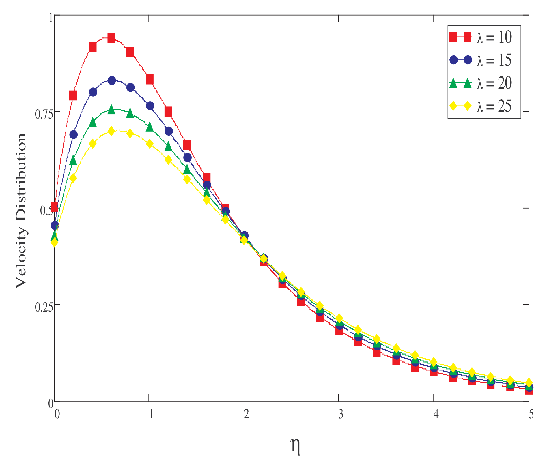
- Rises in the values of Pr, Sc, F, , and slow the fluid’s velocity down.
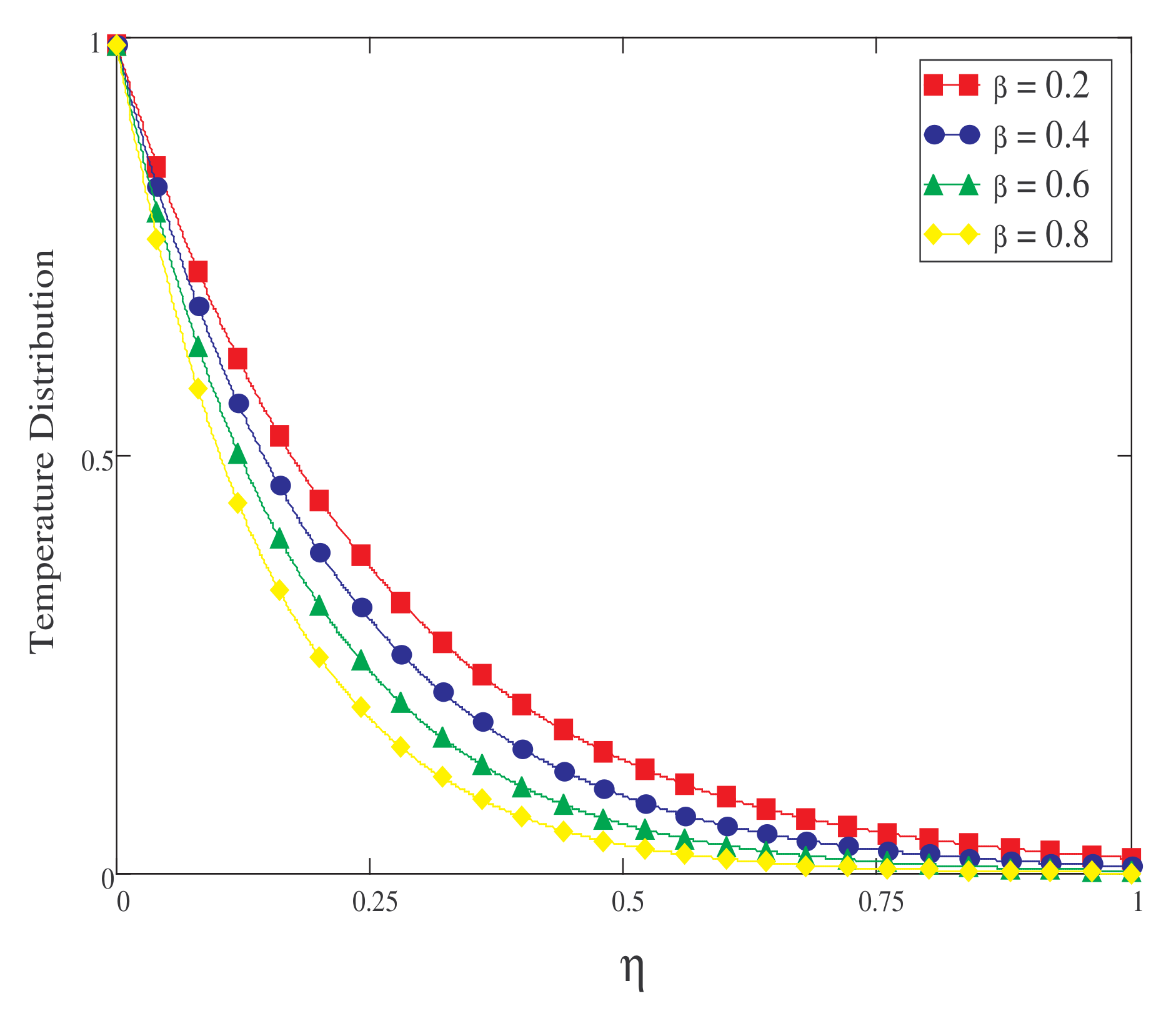
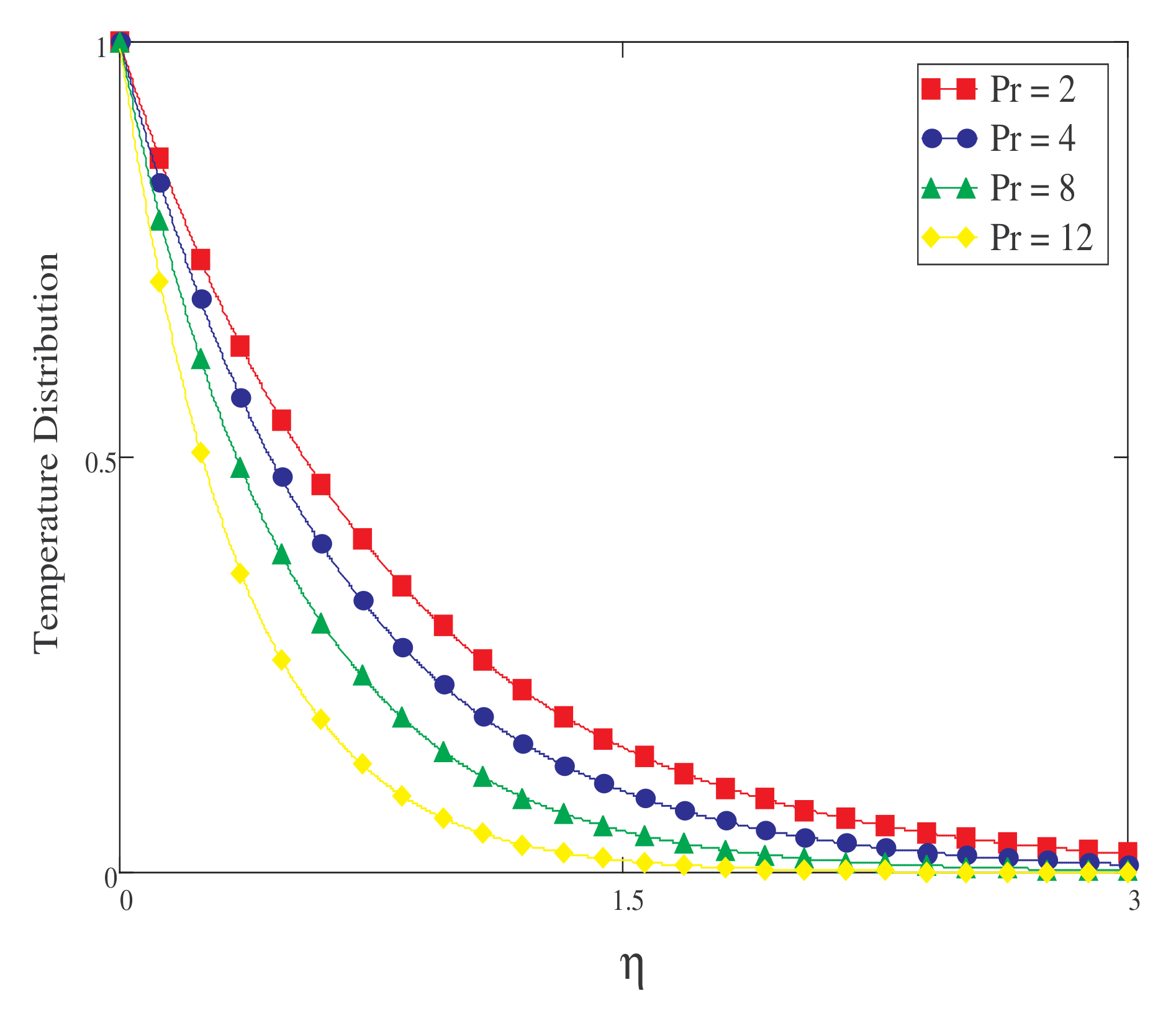
- Rises in the value of Pr decrease the fluid temperature.
- For a short time, the temperature field is a decreasing function of .
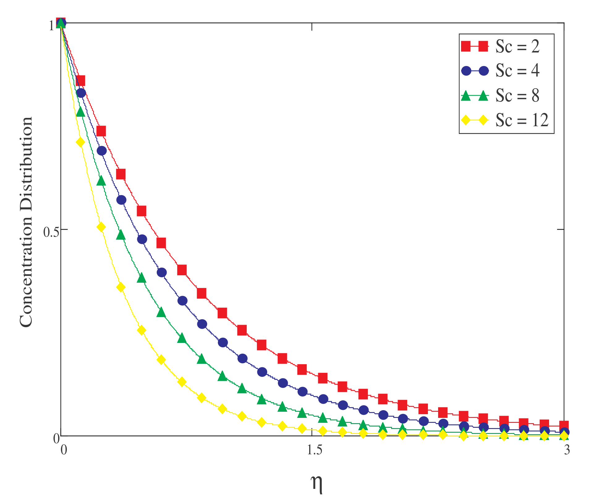
- Increasing the value of Sc decreases the concentration of the fluid.
- For a short time, the concentration field is a decreasing function of .
- The fractionalized outcomes for velocity, temperature, and concentration are generalized and are of a more decaying nature.
Author Contributions
Funding
Data Availability Statement
Acknowledgments
Conflicts of Interest
Nomenclature
| Symbol | Name | Unit |
| U | Velocity of fluid | (m s) |
| u | Velocity of fluid | (m s) |
| T | Temperature of fluid | (K) |
| C | Concentration of fluid | (Kg s) |
| Concentration level at the plate | (Kg m) | |
| Fluid concentration far from the plate | (Kg m) | |
| Temperature of fluid at the plate | (K) | |
| Fluid temperature far away from plate | (K) | |
| Specific heat at constant pressure | (Jkg K) | |
| D | Mass diffusivity | (m s) |
| g | Acceleration due to gravity | (m s) |
| K | Thermal conductivity of fluid | (W m K) |
| Kinematic viscosity of fluid | (m s) | |
| dynamic viscosity | (Kg m s) | |
| Fluid density | (Kg m) | |
| t | Time | (s) |
| Volumetric coefficient of thermal expansion | (K) | |
| Volumetric coefficient of mass expansion | (m Kg) | |
| , | Fractional parameters | (-) |
| M | Magnetic parameter | (-) |
| s | Laplace transform variables | (-) |
| Uniform applied magnetic field | (-) | |
| Jeffrey’s fluid parameter | (-) | |
| Relaxation and retardation time | (-) | |
| Retardation time | (-) | |
| Dimensional chemical reaction parameter | (-) | |
| E | Heat generation | (-) |
| H | Chemical reaction | (-) |
Appendix A
References
- Yang, L.; Du, K. A comprehensive review on the natural, forced, and mixed convection of non-Newtonian fuids (nanofuids) inside different cavities. J. Therm. Anal. Calorim. 2020, 140, 2033–2054. [Google Scholar] [CrossRef]
- Aleem, M.; Asjad, M.I.; Akgul, A. Heat transfer analysis of magnetohydrodynamic Casson fluid through a porous medium with constant proportional Caputo derivative. Heat Transf. 2021, 50, 6444–6464. [Google Scholar] [CrossRef]
- Waqas, H.; Farooq, U.; Liu, D.; Abid, M.; Imran, M.; Muhammad, T. Heat transfer analysis of hybrid nanofluid flow with thermal radiation through a stretching sheet: A comparative study. Int. Commun. Heat Mass Transf. 2022, 138, 106303. [Google Scholar] [CrossRef]
- Ahmad, M.; Asjad, M.I.; Nazar, M. Mathematical modeling of (Cu, Al2O3) water based Maxwell hybrid nanofluids with Caputo-Fabrizio fractional derivative. Adv. Mech. Eng. 2020, 12, 1–11. [Google Scholar] [CrossRef]
- Ayub, R.; Ahmad, S.; Asjad, M.I.; Ahmad, M. Heat transfer analysis for viscous fluid flow with the Newtonian heating and effect of magnetic force in a rotating regime. Complexity 2021, 2021, 9962732. [Google Scholar] [CrossRef]
- Reddy, P.R.; Gaffar, S.A.; Khan, B.M.H.; Venkatadri, K.; Beg, O.A. Mixed convection flows of tangent hyperbolic fluid past an isothermal wedge with entropy: A mathematical study. Heat Transf. 2021, 50, 2895–2928. [Google Scholar] [CrossRef]
- Bajwa, S.; Saif, U.; Al-Johani, A.S.; Khan, I.; Andualem, M. Effects of MHD and porosity on Jeffrey fluid flow with wall transpiration. Math. Probl. Eng. 2022, 2022, 6063143. [Google Scholar] [CrossRef]
- Shafique, A.; Nisa, Z.U.; Asjad, M.I.; Nazar, M.; Jarad, F. Effect of diffusion-thermo on MHD flow of a Jeffrey fluid past an exponentially accelerated vertical plate with chemical reaction and heat generation. Math. Probl. Eng. 2022, 2022, 6279498. [Google Scholar] [CrossRef]
- Krishna, M.V.; Bharathi, K.; Chamkha, A.J. Hall effects on MHD peristaltic flow of Jeffrey fluid through porous medium in a vertical stratum. Interfacial Phenom. Heat Transf. 2018, 6, 241–253. [Google Scholar] [CrossRef]
- Noor, N.A.M.; Shafie, S.; Admon, M.A. Slip effects on MHD squeezing flow of Jeffrey nanofluid in horizontal channel with chemical reaction. Mathematics 2021, 9, 1201–1215. [Google Scholar]
- Siddiqui, A.M.; Farooq, A.A.; Haroon, T.; Babcock, B.S. A variant of the classical von Karman flow for a Jeffrey fluid. Appl. Math. Sci. 2013, 7, 983–991. [Google Scholar] [CrossRef]
- Nadeem, S.; Riaz, A.; Ellahi, R. Peristaltic flow of a Jeffrey fluid in a rectangular duct having compliant walls. Chem. Ind. Chem. Eng. Q. 2013, 19, 399–409. [Google Scholar] [CrossRef]
- Zeeshan, A.; Majeed, A. Heat transfer analysis of Jeffery fluid flow over a stretching sheet with suction/injection and magnetic dipole effect. Alex. Eng. J. 2016, 55, 2171–2181. [Google Scholar] [CrossRef]
- Zin, N.A.M.; Khan, I.; Shafie, S. Influence of thermal radiation on unsteady MHD free convection flow of Jeffrey fluid over a vertical plate with ramped wall temperature. Math. Probl. Eng. 2016, 2016, 6257071. [Google Scholar]
- Kothandapani, M.; Prakash, J. Convective boundary conditions effect on peristaltic flow of a MHD Jeffery nanofluid. Appl. Nanosci. 2016, 6, 323–335. [Google Scholar] [CrossRef]
- Baleanu, D.; Fernandez, A. On fractional operators and their classifications. Mathematics 2019, 7, 830. [Google Scholar] [CrossRef]
- Baleanu, D.; Fernandez, A. On some new properties of fractional derivatives with Mittag-Leffler kernel. Commun. Nonlinear Sci. Numer. Simul. 2018, 59, 444–462. [Google Scholar] [CrossRef]
- Yu, C.H. Fractional derivatives of some fractional functions and their applications. Asian J. Appl. Sci. Technol. 2020, 4, 147–158. [Google Scholar] [CrossRef]
- Hristov, J. Steady-state heat conduction in a medium with spatial non-singular fading memory, derivation of Caputo-Fabrizio space fractional derivative with Jeffreys kernel and analytical solution. Therm. Sci. 2017, 21, 827–839. [Google Scholar] [CrossRef]
- Hristov, J. A transient flow of a non-Newtonian fluid modelled by a mixed time-space derivative: An improved integral-balance approach. In Mathematical Methods in Engineering; Springer: Cham, Switzerland, 2019; pp. 153–174. [Google Scholar]
- Hristov, J. Transient heat diffusion with a non-singular fading memory from the Cattaneo constitutive equation with Jeffrey is kernel to the Caputo-Fabrizio time fractional derivative. Therm. Sci. 2016, 20, 557–562. [Google Scholar] [CrossRef]
- Cruz, F.; Almeida, R.; Martins, N. Optimality conditions for variational problems involving distributed-order fractional derivatives with arbitrary kernels. AIMS Math. 2021, 6, 5351–5369. [Google Scholar] [CrossRef]
- Shafique, A.; Ramzan, M.; Nisa, Z.U.; Nazar, M.; Hafeez, A. Unsteady magnetohydrodynamic flow of second grade Nanofluid (Ag-Cu) with CPC fractional derivative: Nanofluid. J. Adv. Res. Fluid Mech. Therm. Sci. 2022, 97, 103–114. [Google Scholar] [CrossRef]
- El-Nabulsi, R.A. Path integral formulation of fractionally perturbed Lagrangian oscillators on fractal. J. Stat. Phys. 2018, 172, 1617–1640. [Google Scholar] [CrossRef]
- Ahmad, A.; Nazar, M.; Ali, A.; Hussain, M.; Ali, Z. Exact solutions of hydromagnetic fluid flow along an inclined plane with heat and mass trasfer. J. Math. Anal. 2021, 12, 1–12. [Google Scholar]
- Shah, N.A.; Imran, M.A.; Miraj, F. Exact solutions of time fractional free convection flows of viscous fluid over an isothermal vertical plate with Caputo and Caputo-fabrizio derivatives. J. Prime Res. Math. 2017, 13, 56–74. [Google Scholar]
- Jassim, H.K.; Hussain, M.A.S. On approximate solutions for fractional system of differential equations with Caputo-Fabrizio fractional operator. J. Math. Comput. Sci. 2021, 23, 58–66. [Google Scholar] [CrossRef]
- Prasada, R.; Kumarb, K.; Doharec, R. Caputo fractional order derivative model of Zika virus transmission dynamics. J. Math. Comput. Sci. 2023, 28, 145–157. [Google Scholar] [CrossRef]
- Saqib, M.; Ali, F.; Khan, I.; Sheikh, N.A.; Jan, S.A.A. Samiulhaq, Exact solutions for free convection flow of generalized Jeffrey fluid: A Caputo-Fabrizio fractional model. Alex. Eng. J. 2018, 57, 1849–1858. [Google Scholar] [CrossRef]
- Ahmad, M.; Asjad, M.I.; Nisar, K.S.; Khan, I. Mechanical and thermal energies transport flow of a second grade fluid with novel fractional derivative. Proc. Inst. Mech. Eng. Part E 2021. [Google Scholar] [CrossRef]
- Pavlovskii, V.A. On theoretical description of weak aqueous solutions of polymers. Dokl. Akad. Nauk. 1971, 200, 809–812. [Google Scholar]
- Goud, B.S.; Reddy, Y.D.; Mishra, S.R.; Khan, M.I.; Guedri, K.; Galal, A.M. Thermal radiation impact on magneto-hydrodynamic heat transfer micropolar fluid flow over a vertical moving porous plate: A finite difference approach. J. Ind. Chem. Soc. 2022, 99, 100618. [Google Scholar] [CrossRef]
- Biswas, R.; Hossain, M.S.; Islam, R.; Ahmmed, S.F.; Mishra, S.R.; Afikuzzaman, M. Computational treatment of MHD Maxwell nanofluid flow across a stretching sheet considering higher-order chemical reaction and thermal radiation. J. Comput. Math. Data Sci. 2022, 4, 100048. [Google Scholar] [CrossRef]
- Afikuzzaman, M.; Alam, M.M. MHD casson fluid flow through a parallel plate. Sci. Technol. Asia 2016, 21, 59–70. [Google Scholar]
- Oskolkov, A.P. The initial boundary-value problem with a free surface condition for the penalized equations of aqueous solutions of polymers. J. Math. Sci. 1997, 83, 320–326. [Google Scholar] [CrossRef]
- Baranovskii, E.S. Mixed initial-boundary value problem for equations of motion of Kelvin-Voigt fluids. Comput. Math. Math. Phys. 2016, 56, 1363–1371. [Google Scholar] [CrossRef]
- Baleanu, D.; Fernandez, A.; Akgul, A. On a fractional operator combining proportional and classical differintegrals. Mathematics 2020, 360, 360. [Google Scholar] [CrossRef]


Publisher’s Note: MDPI stays neutral with regard to jurisdictional claims in published maps and institutional affiliations. |
© 2022 by the authors. Licensee MDPI, Basel, Switzerland. This article is an open access article distributed under the terms and conditions of the Creative Commons Attribution (CC BY) license (https://creativecommons.org/licenses/by/4.0/).
Share and Cite
Abbas, S.; Nazar, M.; Nisa, Z.U.; Amjad, M.; Din, S.M.E.; Alanzi, A.M. Heat and Mass Transfer Analysis of MHD Jeffrey Fluid over a Vertical Plate with CPC Fractional Derivative. Symmetry 2022, 14, 2491. https://doi.org/10.3390/sym14122491
Abbas S, Nazar M, Nisa ZU, Amjad M, Din SME, Alanzi AM. Heat and Mass Transfer Analysis of MHD Jeffrey Fluid over a Vertical Plate with CPC Fractional Derivative. Symmetry. 2022; 14(12):2491. https://doi.org/10.3390/sym14122491
Chicago/Turabian StyleAbbas, Shajar, Mudassar Nazar, Zaib Un Nisa, Muhammad Amjad, Sayed M. El Din, and Agaeb Mahal Alanzi. 2022. "Heat and Mass Transfer Analysis of MHD Jeffrey Fluid over a Vertical Plate with CPC Fractional Derivative" Symmetry 14, no. 12: 2491. https://doi.org/10.3390/sym14122491
APA StyleAbbas, S., Nazar, M., Nisa, Z. U., Amjad, M., Din, S. M. E., & Alanzi, A. M. (2022). Heat and Mass Transfer Analysis of MHD Jeffrey Fluid over a Vertical Plate with CPC Fractional Derivative. Symmetry, 14(12), 2491. https://doi.org/10.3390/sym14122491