Article

Particle Production in Strong Electromagnetic Fields and Local Approximations

by
Ivan A. Aleksandrov
1,2,*,
Denis G. Sevostyanov
1 and
Vladimir M. Shabaev
1
1
Department of Physics, St. Petersburg State University, 7/9 Universitetskaya Naberezhnaya, 199034 Saint Petersburg, Russia
2
Ioffe Institute, Politekhnicheskaya 26, 194021 Saint Petersburg, Russia
*
Author to whom correspondence should be addressed.
Symmetry 2022, 14(11), 2444; https://doi.org/10.3390/sym14112444
Submission received: 2 November 2022 / Revised: 14 November 2022 / Accepted: 16 November 2022 / Published: 18 November 2022

Abstract

:
We investigate the phenomenon of electron–positron pair production in intense external backgrounds within the strong-field regime. We perform nonperturbative calculations by solving the quantum kinetic equations, and obtain the momentum distributions of particles created and the total number of pairs. In particular, we analyze the validity of the locally constant field approximation (LCFA), which represents a powerful method for treating inhomogeneous external backgrounds. We consider a combination of two consecutive time-dependent Sauter pulses and thoroughly examine the effects of quantum interference and the role of the Pauli exclusion principle. It is shown that the latter can be approximately incorporated within the LCFA when computing the momentum distributions, while the closed-form LCFA expression for the total particle yield completely disregards Pauli blocking. It is demonstrated that in the presence of multiple turning points of classical electron trajectories, one observes interference patterns in the particle spectra, and the LCFA may significantly overestimate the number of pairs. To further elaborate this issue, we perform the analogous calculations in the case of scalar QED. It is shown that the quantum statistics effects enhance the number of bosons produced.

1. Introduction

As it became evident decades ago, a self-consistent theory of electromagnetic interactions should properly incorporate vacuum fluctuations, which can give rise to essentially nonlinear fundamental phenomena, such as light-by-light scattering [1,2,3,4], vacuum birefringence [5,6,7], and electron–positron pair production in strong fields [8,9,10] (for review, see Refs. [11,12,13,14,15,16,17]). The latter process is especially intriguing, as in the case of quasistatic external backgrounds, it can be described only by means of nonperturbative methods. Electron–positron pair production in the strong-field regime (Schwinger mechanism) has never been observed experimentally. From the theoretical viewpoint, it is strongly desirable to explore new setups and obtain accurate predictions concerning various realistic scenarios, as it should significantly facilitate the experimental research.
Since the exact nonperturbative calculations basically require a great amount of computational resources, one has to invoke approximate methods. In this study, we will focus on the widely used locally constant field approximation (LCFA), which allows one to estimate the pair yield in the presence of strong inhomogeneous fields [18,19,20,21,22,23,24,25,26]. The idea here is to employ a closed-form expression for the pair-production probability in the presence of a constant electromagnetic background and then integrate it over space-time, plugging the local values of the actual external-field configuration. In our recent studies [24,25], the validity of the LCFA was explored by comparing the approximate predictions with the results of exact numerical computations. Since the LCFA by definition includes only the tunneling mechanism of pair production, it basically underestimates the exact values. However, in Ref. [25], it was found that the LCFA results may also overestimate the particle number in the case of sufficiently strong external fields. It was suggested that it is the effects of the statistics which are responsible for this nontrivial behavior [25]. Here, we thoroughly examine this issue and discover clear relationships among the LCFA applicability, statistics, and the effects of quantum interference.
In order to simplify the analysis and evidently demonstrate the main mechanisms, we consider a combination of two purely time-dependent pulses. The exact calculations are performed by means of the quantum kinetic equations (QKE) (see Refs. [21,25,26,27,28,29,30,31,32,33]). To properly identify the effects of statistics, we evaluate the momentum distributions of particles and the total pair yield in the case of usual (spinor) quantum electrodynamics and in the case of a scalar field interacting with the classical external background. The process of boson pair production is also investigated by means of the quantum kinetic approach and the LCFA. We employ the units = c = 1 and denote the electron charge by e < 0 . The critical (Schwinger) field strength reads E c = m 2 / | e | .

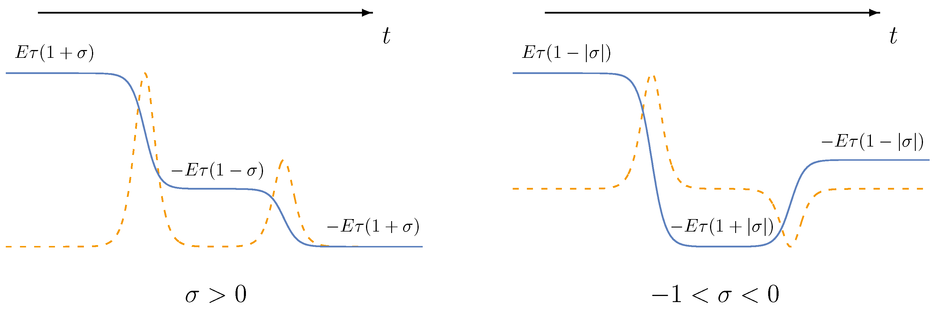
2. External Field Configuration. Turning Points

We assume that the external electric field depends solely on time and has a linear polarization. The field strength is given by the following combination of two Sauter pulses:
E ( t ) = E 1 cosh 2 ( t / τ ) + σ cosh 2 ( t / τ δ ) ,
where τ is the duration of each pulse, E and σ E are the amplitudes of the pulses, and δ governs the temporal distance between the corresponding two peaks. We employ δ = 10 , so the two pulses do not essentially overlap. In the gauge A 0 = 0 , the vector potential reads
A ( t ) = E τ tanh ( t / τ ) + σ tanh ( t / τ δ ) .
As will be demonstrated in what follows, for negative values of σ , one can observe interference effects in the spectra of particles produced. A schematic picture of the external-field profile for positive and negative σ is depicted in Figure 1.
A spatially homogeneous external background is a widely used approximation of the electromagnetic field of two counterpropagating laser pulses forming a standing wave. The pair-production process basically occurs in the vicinity of the electric-field maximum, where the magnetic-field component vanishes. Although laser fields usually contain several optical cycles, here, we consider a very simple model of the external field consisting of Sauter profiles, which can be viewed as very short (half-period) laser pulses. This significantly simplifies the analysis allowing one to clearly identify the main patterns regarding the interference and statistical effects. The general mechanisms revealed in the present study are qualitatively the same, even if the external field has a more involved subcycle structure.
Let us discuss the evolution of the kinetic momentum of the electron in the field E ( t ) . Since the external field does not depend on the spatial coordinates, the generalized momentum P is conserved. Let p = ( p , p ) be the final kinetic momentum of the electron ( p is the momentum projection along the external field direction). From P = p ( t ) + e A ( t ) , it follows that the kinetic momentum as a function of time reads
p ( t ) = p e [ A ( t ) A ( + ) ] .
The perpendicular components do not change, p ( t ) = p . In the nonperturbative regime that we are mostly interested in, the electric field is very unlikely to produce particles with relatively large kinetic energy. Within the LCFA, it is turning point (TP) p ( t * ) = 0 which provides the main contribution to the number density of the electrons (we will discuss the momentum distributions of the electrons, while the positron spectra can be obtained by substituting p p ). In the case of the external field Equation (2) with δ 1 , for any given t, one of the hyperbolic tangents can be replaced with either + 1 or 1 , which simplifies the analysis. For σ > 0 , we obtain the following function t * ( z ) [ z p / ( e E τ ) ]:
t * ( z ) τ = δ + arctanh ( 1 z / σ ) if 0 < z < 2 σ , arctanh ( 1 + 2 σ z ) if 2 σ < z < 2 σ + 2 .
There are no TPs for z outside the interval ( 0 , 2 σ + 2 ) . We also note that Equation (4) is not valid in a certain vicinity of z = 2 σ (this vicinity is exponentially small for large δ ). In what follows, however, the momentum distributions at z = 2 σ will be recovered by simply using their continuity. For 1 < σ < 0 , we can encounter two TPs for given z:
t * ( z ) τ = δ + arctanh ( 1 z / σ ) arctanh ( 1 + 2 σ z ) if 2 σ < z < 0 , arctanh ( 1 + 2 σ z ) if 0 z < 2 σ + 2 .
There are no TPs for z ( 2 σ , 2 σ + 2 ) . The existence of two TPs for certain values of p gives rise to quantum interference that will be investigated in what follows. We will not consider σ < 1 , as this regime is equivalent to the previous one up to interchanging the two pulses and rescaling the amplitude E. Throughout the paper, we will assume E > 0 . Expressions (4) and (5) will be utilized in the following section.

3. Locally Constant Field Approximation

Here, we will briefly recap how the LCFA is implemented for computing the particle spectra and total number of pairs (see also Refs. [24,25]).

3.1. Momentum Distributions

Let us first describe how one can evaluate the dimensionless number density of electrons defined via
f ( p ) = ( 2 π ) 3 V d N p , s d p ,
where V is the volume of the system and s governs the spin state of the particle produced. In our case, the results do not depend on s, so one can simply double f ( p ) to take into account the spin degeneracy. As the external field is homogeneous in space, we evaluate the number density of particles per unit volume. The momentum distribution Equation (6) at any given p cannot exceed unity according to the Pauli principle.
In order to estimate the number density Equation (6), we will first propagate the electron momentum p backwards in time according to Equation (3) and determine the TP(s) Equation (4) or (5) depending on the sign of σ . The idea of the LCFA is to employ then the well-known expression for the pair-production probability density in a constant electric field E [10],
W ( p ) = exp π π 2 | e E | ,
where π m 2 + p 2 . Within the LCFA, one evaluates Equation (7) using the field amplitude at the corresponding TP. In the case σ > 0 , where there is always no more than one TP for given p , we obtain the following LCFA prediction for the particle number density:
f σ > 0 ( LCFA ) ( p ) = F ( E ; p , p + 2 σ | e E | τ ) if 2 ( σ + 1 ) | e E | τ < p < 2 σ | e E | τ , F ( σ E ; p , p ) if 2 σ | e E | τ < p < 0 , 0 otherwise ,
where
F ( E ; p , p ) = exp π π 2 | e E | τ 2 p ( p 2 e E τ ) .
Note that z = 2 σ in Equation (4) corresponds to p = 2 σ | e E | τ , which yields a zero value of f σ > 0 ( LCFA ) ( p ) , and the piecewise expression (8) is a continuous function. Taking a closer look at Equation (8), one can easily find out that this distribution represents two separate bell-shaped profiles, whose physical interpretation is clear: the first Sauter pulse in Equation (1) creates electrons with a bell-shaped momentum distribution; these particles are then accelerated by the second Sauter pulse, which also generates electrons described by the second line in Equation (8). Accordingly, the first line in Equation (8) includes the shift 2 σ | e E | τ and involves the different field amplitude. The two Sauter pulses create pairs independently. As was demonstrated in Refs. [24,25], in the case of an individual Sauter pulse of amplitude E and duration τ , the LCFA is accurate if | e E | 3 / 2 τ m 2 . This means that Equation (8) provides accurate predictions if | e E | 3 / 2 τ m 2 and | σ e E | 3 / 2 τ m 2 simultaneously. As will be seen below, the case σ < 0 is much less trivial. It is the main focus of our study.
As was indicated above, in the case σ < 0 some values of p correspond to two TPs. The easiest way to treat them is to simply sum the corresponding probabilities W ( p ) , which brings us to
f σ < 0 ( LCFA ) ( p ) = F ( E ; p , p 2 | σ e E | τ ) if 2 ( σ + 1 ) | e E | τ < p 0 , F ( E ; p , p 2 | σ e E | τ ) + F ( σ E ; p , p ) if 0 < p < 2 | σ e E | τ , 0 otherwise .
Nevertheless, this simple prescription is obviously incorrect, as it does not prevent the number density from exceeding unity with the increasing number of TPs. In order to take into account the Pauli exclusion principle, one has to multiply the contribution from the second TP by a suppressing factor since the electron cannot be produced at the second TP if the corresponding state is already occupied by the particle created at the first TP. The correct implementation of the LCFA reads [25,34,35]
f σ < 0 ( LCFA + ) ( p ) = F ( E ; p , p 2 | σ e E | τ ) if 2 ( σ + 1 ) | e E | τ < p 0 , G ( E , σ ; p , p ) if 0 < p < 2 | σ e E | τ , 0 otherwise ,
where
G ( E , σ ; p , p ) = F ( E ; p , p 2 | σ e E | τ ) + [ 1 2 F ( E ; p , p 2 | σ e E | τ ) ] F ( σ E ; p , p ) .
Here the second term contains suppressing factor 1 2 F . This scheme can easily be generalized in the case of many TPs, and it always yields number densities less than unity. We label this approach as LCFA+ and in what follows, we will employ both this approximation and the “naive” LCFA version Equation (10). In the case of scalar QED, one should change the sign of the 2 F term in Equation (12) so that the statistical factor enhances the number of bosons produced. Note that the LCFA and LCFA+ can differ only if the effects of statistics become important. This issue will be investigated in detail.

3.2. Total Number of Pairs

Within the LCFA, in order to evaluate the total number of pairs, which obviously coincides with the total number of electrons or positrons, one has to integrate the momentum distribution Equation (8) for σ > 0 or Equation (10) for σ < 0 . However, in this section, we will consider a generic time-dependent background E ( t ) . Let us first assume that the corresponding potential A ( t ) is monotonous, i.e., the number of TPs is either 0 or 1 for any given p . The total number of pairs is given by
( 2 π ) 3 V N ( LCFA ) = 2 d p exp π π 2 | e E ( t * ) | .
Here, one integrates over p Π where the electron trajectories have TPs. We have also introduced a factor of 2 due to spin degeneracy. Note that within Π we have a one-to-one correspondence between p and t * since the vector potential is monotonous. It allows one to substitute p with t * by using Equation (3) [ d p = e E ( t * ) d t * ] and obtain
( 2 π ) 3 V N ( LCFA ) = 4 π 0 d p p d t | e E ( t ) | exp π ( m 2 + p 2 ) | e E ( t ) | = 2 e 2 E 2 ( t ) exp π m 2 | e E ( t ) | .
If the vector potential A ( t ) is not monotonous, i.e., the field strength E ( t ) can change its sign, one can split the p axis into intervals of constant E sign and straightforwardly demonstrate that summing over all of the TPs leads again to Equation (14). Note that the contributions arising from different TPs are directly combined according to the simple LCFA prescription used in Equation (10), i.e., no statistical effects are taken here into account.
In Equation (14), one explicitly sums the local contributions from each small time interval [ t , t + Δ t ] . Alternatively, one can employ a closed-form expression for the total number of pairs produced per unit volume and time in a constant electric field [36,37]. Plugging the actual temporal dependence E ( t ) into this expression, one obtains exactly the same formula as (14) (see Refs. [18,19,20,21,22,23,24,25,26]). Note that the LCFA expression (14) can easily be generalized in order to consider arbitrary space-time-dependent backgrounds, while the TP analysis performed in the previous subsection is no longer valid in the case of multidimensional inhomogeneities [24].
It is clear that there is no point in integrating the LCFA momentum spectra f ( LCFA ) ( p ) , as one can instead perform one-dimensional integration Equation (14). Nevertheless, to approximately take into account the effects of statistics as was done within the LCFA+ in the previous section, one has to integrate the momentum distribution f ( LCFA + ) ( p ) . The statistical factor 1 2 F (or 1 + 2 F for bosons) in Equation (12) is essentially nonlocal, so it is not possible to deduce a closed-form LCFA expression for the total particle yield which incorporates the statistics of the particles produced. We will directly integrate the number density Equation (11) over p and also refer to the corresponding results as the LCFA+. Finally, we point out that in the case of scalar QED, the LCFA expression (14) remains the same apart from the spin factor 2 (see Ref. [37]).

4. Quantum Kinetic Equations

In this section, we will briefly outline the method based on solving the QKE [21,25,26,27,28,29,30,31,32,33]. It allows one to accurately obtain the distribution function Equation (6) treating the temporal dependence of the classical external field without any additional approximations. This technique precisely takes into account quantum interference and the effects of statistics. It is exact to the zeroth order in the radiative interaction, i.e., the photon degrees of freedom are entirely disregarded.
Let us assume that the external background E ( t ) vanishes for t < t in and t > t out (in our case, t in / out ). The electron distribution function Equation (6) coincides with the asymptotic values of the adiabatic particle number density f ( p , t ) for t > t out . The latter can be found via
f ˙ ( p , t ) = λ ( p , t ) t in t d t λ ( p , t ) 1 2 f ( p , t ) cos 2 θ ( t , t ) ,
where
λ ( p , t ) = e E ( t ) π ω 2 ( p , t ) ,
ω ( p , t ) = π 2 + [ p e A ( t ) ] 2 ,
θ ( t , t ) = t t ω ( p , t ) d t .
The initial condition reads f ( p , t in ) = 0 for all p . Instead of using Equation (15), it is basically more convenient to solve the following equivalent system of differential equations:
f ˙ ( p , t ) = 1 2 λ ( p , t ) u ( p , t ) ,
u ˙ ( p , t ) = 1 2 f ( p , t ) λ ( p , t ) 2 ω ( p , t ) v ( p , t ) ,
v ˙ ( p , t ) = 2 ω ( p , t ) u ( p , t ) .
Here, we also set u ( p , t in ) = v ( p , t in ) = 0 for all p . The system Equations (19)–(21) is referred to as the quantum kinetic equations (QKE). Note that a more general system can be employed for describing pair production in uniform electric fields of arbitrary polarization (see Ref. [33] and the references therein). We also point out that the abiabatic number density f ( p , t ) does not yield the physical number of particles at intermediate times t ( t in , t out ) (see recent studies [26,38]). The function u ( p , t ) determines the polarization current, and the function v ( p , t ) describes the energy density of the vacuum polarization [33] (see also Ref. [39]). We will solve the system Equations (19)–(21) numerically in the case of the external background Equation (1) and compare the results with the approximate predictions obtained within the LCFA and LCFA+.
Equation (20) contains factor 1 2 f ( p , t ) , which reflects the Fermi statistics of electrons. Here, one can argue that for sufficiently weak external fields, this factor does not differ much from unity, so one can approximately omit the function f ( p , t ) in the right-hand side of Equations (20) and (15). This approach is called the low-density approximation (LDA) [21,30,32] which will also be utilized in our study. It turns out that within the LDA, one can easily integrate Equation (15):
f ( LDA ) ( p ) = 1 4 | t in t out λ ( p , t ) e 2 i θ ( t , t in ) d t | 2 .
In the case of scalar QED, the function λ ( p , t ) should be defined via λ ( p , t ) = e E ( t ) [ p e A ( t ) ] / ω 2 ( p , t ) , and one has to change the sign in the square brackets in Equation (20), so that the factor reads 1 + 2 f ( p , t ) .

5. Results

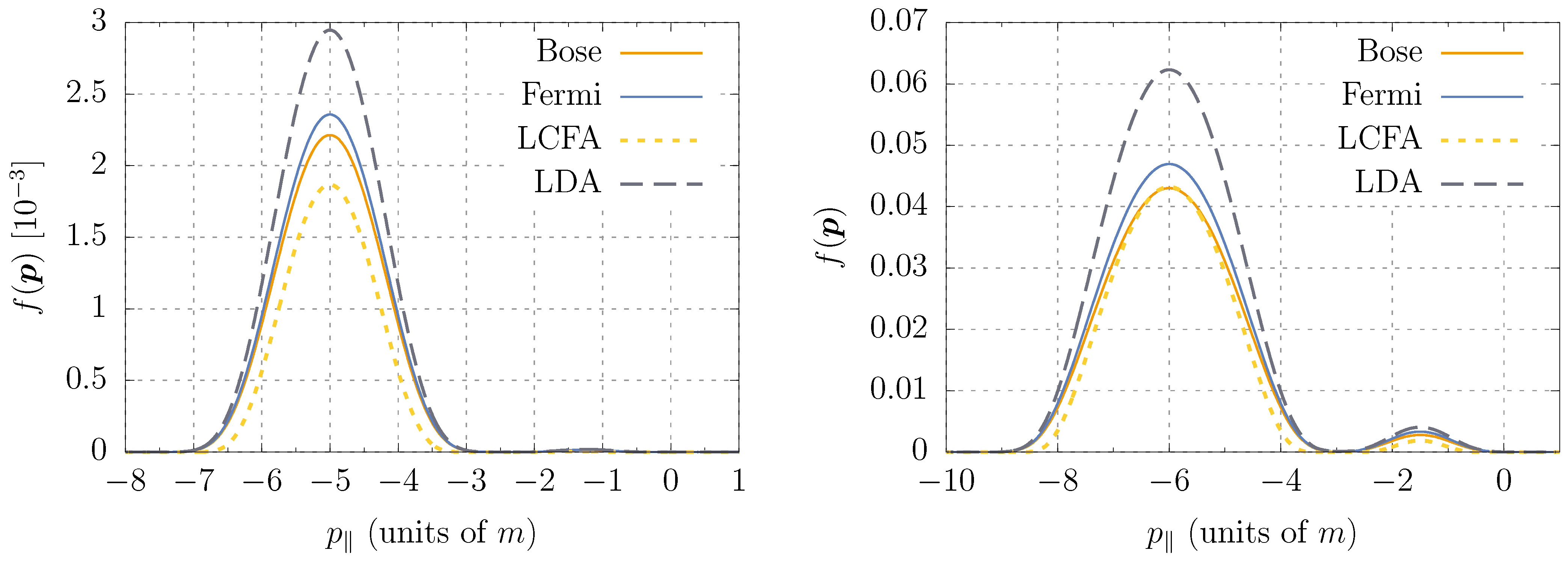
5.1. Momentum Distributions for Positive
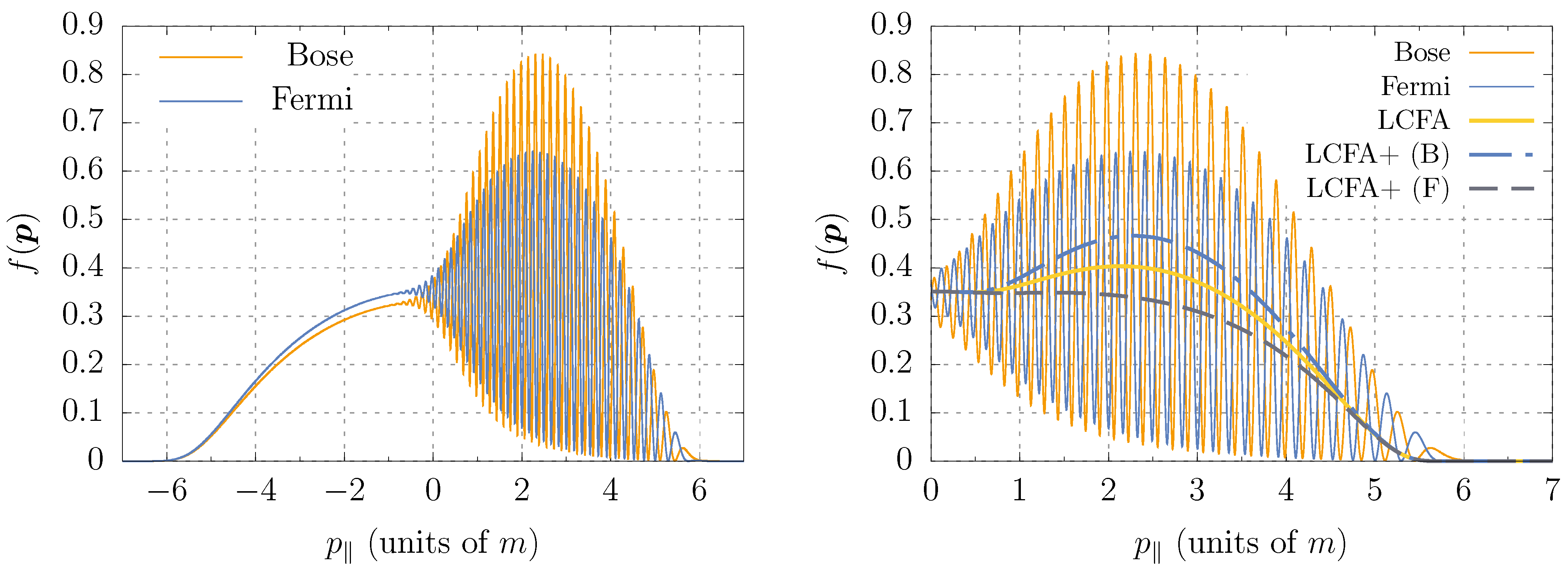
 σ

Let us first address the case σ > 0 , where there is no more than one TP and the LCFA prediction (8) for the momentum distribution consists of two separate bell-shaped profiles. In Figure 2, we present two examples of the particle spectra computed by means of the QKE (solid lines), LCFA (yellow dashed lines), and LDA for fermions (grey dashed lines). According to Equation (8), the LCFA predicts two bell-shaped profiles centered at p = ( 2 σ + 1 ) | e E | τ and p = σ | e E | τ , respectively (the second peak in the left panel is hardly visible due to the small number densities as the amplitude σ E appears to be too low compared to E in this case). We observe that the exact and approximate techniques yield exactly the same support of the momentum distributions and the peak positions. However, the number densities are different. First, we note that the exact number densities evaluated in the case of scalar QED are smaller than those computed for electrons. This can be found already for an individual Sauter pulse, i.e., σ = 0 . In this case, one can employ the exact closed-form expressions for f ( p ) (see Ref. [40]). It turns out that the ratio of the maximal number densities calculated for bosons and fermions amounts to
R max f ( p ) ( Bose ) max f ( p ) ( Fermi ) = cosh 2 ( π ( ξ m τ ) 2 1 / 4 ) sinh 2 ( π ξ m τ ) ,
where ξ = | e E | τ / m is a classical adiabaticity parameter. The nonperturbative regime of pair production corresponds to ξ 1 . In the case ξ m τ 1 , one obtains
R exp π 4 1 ξ m τ .
This means that R < 1 and this ratio is close to 1 in the domain of sufficiently large ξ m τ . A relative difference of 5 % ( R = 0.95 ) corresponds to ξ m τ 15.3 . In Figure 2, the stronger Sauter pulse has ξ m τ = 12.5 (left panel) and ξ m τ = 9 (right panel). Accordingly, for larger values of E and τ , the spinor-QED and scalar-QED results in the case of an individual Sauter pulse will be closer to each other. For σ > 0 , we have essentially a pair of independent Sauter pulses, so the same condition holds true in our case. Moreover, one can straightforwardly confirm that a single Sauter pulse produces particles with exactly the same momentum distributions, once one takes into account the corresponding momentum shifts in the field of the second pulse. This means that for σ > 0 , it suffices to consider an individual Sauter pulse and examine the local approximations for this simpler field configuration. This was verified in Ref. [24] (see also Ref. [25]), where it was found that the LCFA accurately reproduces the exact spectra if | e E | 3 / 2 τ m 2 . The field parameters chosen in Figure 2 yield for the stronger pulse | e E | 3 / 2 τ 1.8 m 2 (left panel) and | e E | 3 / 2 τ 3 m 2 (right panel), so the LCFA is not completely justified, although it definitely provides adequate estimates. Note that the LCFA predictions for σ > 0 never exceed the exact number densities [24,25]. As will be shown in what follows, negative values of σ lead to much fewer trivial momentum spectra. For instance, the ratio R will not tend to unity for large E due to the effects of statistics, which do not manifest themselves for σ > 0 . Finally, Figure 2 reveals that the LDA can considerably overestimate the electron number density, even if the latter itself is much smaller than unity. In fact, the LDA is indeed accurate for lower field amplitudes, E 0.1 E c . We also confirmed that the validity of the LDA is almost independent of τ , provided the pulse duration is sufficiently large [21].

5.2. Negative σ . Interference Effects

According to Equation (5), in the case σ < 0 , particle longitudinal momenta p within the interval ( 0 , 2 | σ e E | τ ) correspond to two TPs. It means that such particle can be produced by either pulse, which leads to quantum interference of the two possible events [24,25,31,41,42,43,44,45,46].
As an example, we choose σ = 1 / 2 , so the support of the momentum distribution is symmetric, p ( | e E | τ , | e E | τ ) , and the interference effects should be revealed within the positive- p region. In Figure 3, we present the results of exact calculations in the case of bosons and fermions (solid lines) and the approximate predictions obtained with the aid of the LCFA and LCFA+ (see right panel). In the left panel, we observe a very nontrivial behavior showing that the relation between the spinor-QED and scalar-QED predictions is twofold. On the one hand, the number density at the vicinity of p = 0 is again smaller in the case of bosons according to our estimate (24). With increasing E, this difference vanishes. On the other hand, the oscillatory structure of the momentum distribution is not only more pronounced for Bose particles, but also leads to larger values of the boson yield (aside from the spin factor 2, which always double the number of electrons). It suggests that the effects of statistics can lead to a notable enhancement of scalar–particle production, whereas the Pauli exclusion principle only inhibits the creation of electron–positron pairs in the domain of high-field amplitudes. This issue will also be examined in the next section, where we will analyze the total number of particles produced. We also note that the frequency of the oscillations in Figure 3 is proportional to τ and δ as can be verified by direct numerical calculations with different field parameters or by means of the semiclassical analysis (see Ref. [44]).
Since within the LCFA and LCFA+ one combines the contributions arising from different TPs on the level of probabilities, the effects of quantum interference in the particle spectra are completely neglected within these approximations as we clearly see in the right panel of Figure 3. Nevertheless, the LCFA may provide a reasonable estimate for a “mean curve” and thus accurately predict the total amount of pairs. Here it can be important to take into account the statistics effects by means of the LCFA+, as the basic LCFA tends to overestimate (underestimate) the pair-production probabilities in the case of fermions (bosons).
We also point out that the LDA spectra (not shown here) possess interference patterns but may yield inaccurate quantitative estimates. As we are mainly interested here in the effects of statistics in strong pulses ( E 0.1 E c ), the LDA is always significantly less accurate than the LCFA and LCFA+. In what follows, we will calculate the total number of pairs by means of the various techniques.

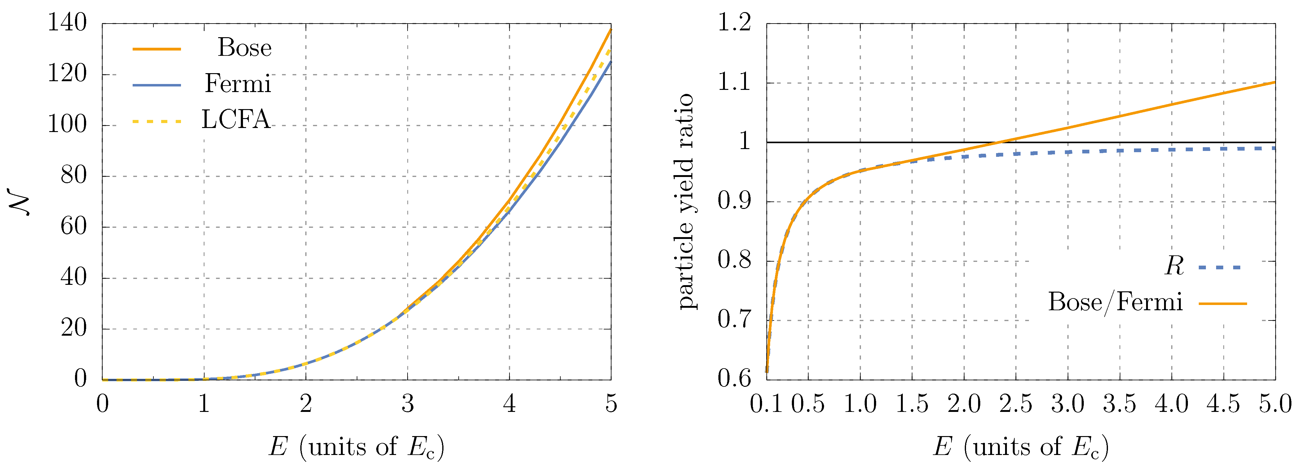
5.3. Total Number of Particles

In this section, we will always multiply the total number of bosons by a factor of two in order to compare the results without considering the trivial effect of spin degeneracy in the case of fermions.
In Figure 4 (left panel), we display the quantity N = ( 2 π ) 3 N / V as a function of E for σ = 1 / 2 , τ = 4 m 1 , and δ = 10 . First, one observes that the number of bosons exceeds the number of fermions for sufficiently large field amplitudes. Since the ratio Equation (24) tends to 1, this feature appears due to the statistics effects. This point is evidently demonstrated in the right panel of Figure 4, where we present the ratio of the Bose and Fermi yields together with the function Equation (24). For relatively low field amplitudes, our estimate Equation (24) perfectly describes the quantitative difference between the pair production processes of bosons and fermions. Since the support of the momentum distribution is the same, the ratio of Equation (23) coincides with the ratio of the total particle yields. However, for sufficiently large E, the number of fermions becomes smaller than the number of bosons due to the effects of statistics. Moreover, we observe that the LCFA predictions in the strong-field domain overestimate the electron number as they do not incorporate the Pauli principle. On the other hand, the LCFA underestimates the total yield of scalar particles since Bose statistics leads to the additional enhancement of pair production. We also note that for lower amplitudes, the validity of the LCFA is governed again by the criterion | e E | 3 / 2 τ m 2 . For instance, for E = 0.2 E c this parameter amounts to | e E | 3 / 2 τ 0.36 m 2 and the LCFA predictions are about two orders of magnitude smaller than the actual particle yield (it is not visible in Figure 4 due to the linear scale of the N axis).
The effects of statistics can be taken into account by means of the LCFA+. Although the LCFA uncertainty increases with E, the LCFA+ becomes more accurate. For example, at E = 5 E c in the case of bosons, the relative uncertainty of the LCFA is about 5 % while the uncertainty of the LCFA+ is less than 0.1 % .
According to the previous section, the effects of statistics manifest themselves only in the presence of quantum interference. This can also be confirmed by computing the total number of pairs in the case of positive σ . We performed analogous calculations for σ = 1 / 2 . Although the LCFA predictions remain the same, as they do not depend on the sign of σ , these approximate results are now always smaller than the exact number of bosons and fermions. The ratio of the latter particle numbers coincides with the expression (24) and tends to unity with increasing E. These observations demonstrate that statistics plays an important role if (a) the pair-production process involves quantum interference, (b) the field amplitude is sufficiently high, so the external background produces a significant amount of pairs.

6. Discussion

In the present study, we considered a simple configuration of the external electric field and investigated the effects of quantum interference and the role of particle statistics in the context of vacuum pair production. Special focus was placed on the analysis of the LCFA accuracy for computing the particle momentum distributions and total number of pairs. By performing exact calculations within the quantum kinetic approach, it was shown that the local approximation can be invalid even if the field amplitude is large. Moreover, the corresponding discrepancy, which appears due to the effects of statistics, increases with the field strength. It turns out that this behavior can be observed only in the presence of the interference effects in the particle momentum spectra, i.e., these two phenomena accompany each other and occur if the classical trajectories of the charged particles have multiple turning points. We note that the mechanisms uncovered in the present study can have different quantitative features depending on the external-field parameters. For instance, in the case of many turning points, the interference and statistics effects will be more pronounced. This issue is relevant to possible experimental investigations, as the realistic scenarios involving laser pulses can easily possess a large number of oscillations.

Author Contributions

Conceptualization, methodology, investigation, and writing, I.A.A., D.G.S. and V.M.S.; software, I.A.A. and D.G.S. All authors have read and agreed to the published version of the manuscript.

Funding

This research was funded by RFBR and ROSATOM, grant number 20-21-00098. I.A.A. acknowledges the support from the Foundation for the advancement of theoretical physics and mathematics “BASIS”.

Data Availability Statement

Not applicable.

Conflicts of Interest

The authors declare no conflict of interest.

Abbreviations

The following abbreviations are used in this manuscript:
QEDQuantum electrodynamics
LCFALocally constant field approximation
QKEQuantum kinetic equations
TPTurning point

References

  1. Euler, H.; Kockel, B. Über die Streuung von Licht an Licht nach der Diracschen Theorie. Naturwissenschaften 1935, 23, 246–247. [Google Scholar] [CrossRef]
  2. Weisskopf, V. Über die Elektrodynamik des Vakuums auf Grund der Quantentheorie des Elektrons. Kong. Dan. Vid. Sel. Mat. Fys. Med. 1936, XIV, 1–39. [Google Scholar]
  3. Karplus, R.; Neuman, M. Non-linear interactions between electromagnetic fields. Phys. Rev. 1950, 80, 380–385. [Google Scholar] [CrossRef]
  4. Karplus, R.; Neuman, M. The scattering of light by light. Phys. Rev. 1951, 83, 776–784. [Google Scholar] [CrossRef]
  5. Baier, R.; Breitenlohner, P. Photon propagation in external fields. Act. Phys. Austriaca 1967, 25, 212. [Google Scholar]
  6. Baier, R.; Breitenlohner, P. The vacuum refraction index in the presence of external fields. Nuovo Cimento B 1967, 47, 117–120. [Google Scholar] [CrossRef]
  7. Aleksandrov, E.B.; Ansel’m, A.A.; Moskalev, A.N. Vacuum birefringence in an intense laser radiation field. Zh. Eksp. Teor. Fiz. 1985, 62, 1181, Translated: Sov. Phys. JETP 1985, 62, 680. [Google Scholar]
  8. Sauter, F. Über das Verhalten eines Elektrons im homogenen elektrischen Feld nach der relativistischen Theorie Diracs. Z. Phys. 1931, 69, 742–764. [Google Scholar] [CrossRef]
  9. Heisenberg, W.; Euler, H. Folgerungen aus der Diracschen Theorie des Positrons. Z. Phys. 1936, 98, 714–732. [Google Scholar] [CrossRef]
  10. Schwinger, J. On gauge invariance and vacuum polarization. Phys. Rev. 1951, 82, 664–679. [Google Scholar] [CrossRef]
  11. Dunne, G.V. New strong-field QED effects at extreme light infrastructure. Eur. Phys. J. D 2009, 55, 327. [Google Scholar] [CrossRef] [Green Version]
  12. Heinzl, T.; Ilderton, A. Exploring high-intensity QED at ELI. Eur. Phys. J. D 2009, 55, 359. [Google Scholar] [CrossRef]
  13. Marklund, M.; Lundin, J. Quantum vacuum experiments using high intensity lasers. Eur. Phys. J. D 2009, 55, 319. [Google Scholar] [CrossRef]
  14. Di Piazza, A.; Müller, C.; Hatsagortsyan, K.Z.; Keitel, C.H. Extremely high-intensity laser interactions with fundamental quantum systems. Rev. Mod. Phys. 2012, 84, 1177–1228. [Google Scholar] [CrossRef] [Green Version]
  15. Blaschke, D.; Gevorgyan, N.T.; Panferov, A.D.; Smolyansky, S.A. Schwinger effect at modern laser facilities. J. Phys. Conf. Ser. 2016, 672, 012020. [Google Scholar] [CrossRef] [Green Version]
  16. Xie, B.S.; Li, Z.L.; Tang, S. Electron-positron pair production in ultrastrong laser fields. Matter Radiat. Extremes. 2017, 2, 225–242. [Google Scholar] [CrossRef] [Green Version]
  17. Fedotov, A.; Ilderton, A.; Karbstein, F.; King, B.; Seipt, D.; Taya, H.; Torgrimsson, G. Advances in QED with intense background fields. arXiv 2022, arXiv:2203.00019. [Google Scholar]
  18. Bunkin, F.V.; Tugov, I.I. The possibility of electron-positron pair production in vacuum when laser radiation is focussed. Dokl. Akad. Nauk SSSR 1969, 187, 541–544, Translated: Sov. Phys. Dokl. 1970, 14, 678. [Google Scholar]
  19. Narozhny, N.B.; Bulanov, S.S.; Mur, V.D.; Popov, V.S. e+e-pair production by a focused laser pulse in vacuum. Phys. Lett. A 2004, 330, 1–6. [Google Scholar] [CrossRef] [Green Version]
  20. Dunne, G.V.; Wang, Q.; Gies, H.; Schubert, C. Worldline instantons and the fluctuation prefactor. Phys. Rev. D 2006, 73, 065028. [Google Scholar] [CrossRef] [Green Version]
  21. Hebenstreit, F.; Alkofer, R.; Gies, H. Pair production beyond the Schwinger formula in time-dependent electric fields. Phys. Rev. D 2008, 78, 061701(R). [Google Scholar] [CrossRef] [Green Version]
  22. Bulanov, S.S.; Mur, V.D.; Narozhny, N.B.; Nees, J.; Popov, V.S. Multiple colliding electromagnetic pulses: A way to lower the threshold of e+e pair production from vacuum. Phys. Rev. Lett. 2010, 104, 220404. [Google Scholar] [CrossRef] [Green Version]
  23. Gavrilov, S.P.; Gitman, D.M. Vacuum instability in slowly varying electric fields. Phys. Rev. D 2017, 95, 076013. [Google Scholar] [CrossRef] [Green Version]
  24. Aleksandrov, I.A.; Plunien, G.; Shabaev, V.M. Locally-constant field approximation in studies of electron-positron pair production in strong external fields. Phys. Rev. D 2019, 99, 016020. [Google Scholar] [CrossRef] [Green Version]
  25. Sevostyanov, D.G.; Aleksandrov, I.A.; Plunien, G.; Shabaev, V.M. Total yield of electron-positron pairs produced from vacuum in strong electromagnetic fields: Validity of the locally constant field approximation. Phys. Rev. D 2021, 104, 076014. [Google Scholar] [CrossRef]
  26. Aleksandrov, I.A.; Sevostyanov, D.G.; Shabaev, V.M. Schwinger particle production: Rapid switch off of the external field versus dynamical assistance. arXiv 2022, arXiv:2210:15626. [Google Scholar]
  27. Grib, A.A.; Mamaev, V.M.; Mostepanenko, V.M. Vacuum Quantum Effects in Strong External Fields; Friedmann Laboratory Publishing: St. Petersburg, Russia, 1994. [Google Scholar]
  28. Schmidt, S.M.; Blaschke, D.; Röpke, G.; Smolyansky, S.A.; Prozorkevich, A.V.; Toneev, V.D. A quantum kinetic equation for particle production in the Schwinger mechanism. Int. J. Mod. Phys. E 1998, 7, 709–722. [Google Scholar] [CrossRef] [Green Version]
  29. Kluger, Y.; Mottola, E.; Eisenberg, J.M. Quantum Vlasov equation and its Markov limit. Phys. Rev. D 1998, 58, 125015. [Google Scholar] [CrossRef] [Green Version]
  30. Schmidt, S.; Blaschke, D.; Röpke, G.; Prozorkevich, A.V.; Smolyansky, S.A.; Toneev, V.D. Non-Markovian effects in strong-field pair creation. Phys. Rev. D 1999, 59, 094005. [Google Scholar] [CrossRef] [Green Version]
  31. Hebenstreit, F.; Alkofer, R.; Dunne, G.V.; Gies, H. Momentum signatures for Schwinger pair production in short laser pulses. Phys. Rev. Lett. 2009, 102, 150404. [Google Scholar] [CrossRef] [Green Version]
  32. Fedotov, A.M.; Gelfer, E.G.; Korolev, K.Y.; Smolyansky, S.A. Kinetic equation approach to pair production by a time-dependent electric field. Phys. Rev. D 2011, 83, 025011. [Google Scholar] [CrossRef] [Green Version]
  33. Aleksandrov, I.A.; Dmitriev, V.V.; Sevostyanov, D.G.; Smolyansky, S.A. Kinetic description of vacuum e+e production in strong electric fields of arbitrary polarization. Eur. Phys. J. Spec. Top. 2020, 229, 3469–3485. [Google Scholar] [CrossRef]
  34. Kluger, Y.; Eisenberg, J.M.; Svetitsky, B.; Cooper, F.; Mottola, E. Pair production in a strong electric field. Phys. Rev. Lett. 1991, 67, 2427–2430. [Google Scholar] [CrossRef]
  35. Kluger, Y.; Eisenberg, J.M.; Svetitsky, B.; Cooper, F.; Mottola, E. Fermion pair production in a strong electric field. Phys. Rev. D 1992, 45, 4659–4671. [Google Scholar] [CrossRef] [Green Version]
  36. Nikishov, A.I. Pair production by a constant external field. Zh. Eksp. Teor. Fiz. 1969, 57, 1210, Translated: Sov. Phys. JETP 1970, 30, 660. [Google Scholar]
  37. Fradkin, E.S.; Gitman, D.M.; Shvartsman, S.M. Quantum Electrodynamics with Unstable Vacuum; Springer: Berlin, Germany, 1991. [Google Scholar]
  38. Ilderton, A. Physics of adiabatic particle number in the Schwinger effect. Phys. Rev. D 2022, 105, 016021. [Google Scholar] [CrossRef]
  39. Aleksandrov, I.A.; Panferov, A.D.; Smolyansky, S.A. Radiation signal accompanying the Schwinger effect. Phys. Rev. A 2021, 103, 053107. [Google Scholar] [CrossRef]
  40. Gavrilov, S.P.; Gitman, D.M. Vacuum instability in external fields. Phys. Rev. D 1996, 53, 7162–7175. [Google Scholar] [CrossRef] [Green Version]
  41. Dumlu, C.K.; Dunne, G.V. Stokes phenomenon and Schwinger vacuum pair production in time-dependent laser pulses. Phys. Rev. Lett. 2010, 104, 250402. [Google Scholar] [CrossRef] [Green Version]
  42. Dumlu, C.K.; Dunne, G.V. Interference effects in Schwinger vacuum pair production for time-dependent laser pulses. Phys. Rev. D 2011, 83, 065028. [Google Scholar] [CrossRef] [Green Version]
  43. Dumlu, C.K.; Dunne, G.V. Complex worldline instantons and quantum interference in vacuum pair production. Phys. Rev. D 2011, 84, 125023. [Google Scholar] [CrossRef] [Green Version]
  44. Akkermans, E.; Dunne, G.V. Ramsey fringes and time-domain multiple-slit interference from vacuum. Phys. Rev. Lett. 2012, 108, 030401. [Google Scholar] [CrossRef] [PubMed] [Green Version]
  45. Aleksandrov, I.A.; Plunien, G.; Shabaev, V.M. Pulse shape effects on the electron-positron pair production in strong laser fields. Phys. Rev. D 2017, 95, 056013. [Google Scholar] [CrossRef] [Green Version]
  46. Aleksandrov, I.A.; Kohlfürst, C. Pair production in temporally and spatially oscillating fields. Phys. Rev. D 2020, 101, 096009. [Google Scholar] [CrossRef]
Figure 1. Temporal dependence of the external field Equation (1) (dashed lines) and vector potential Equation (2) (solid lines) in the case of positive (left) and negative (right) values of the parameter σ . In the latter case, the vector potential is not monotonous, so the classical electron trajectory can have two turning points.
Symmetry 14 02444 g001
Figure 2. Momentum distributions of negatively charged fermions and bosons produced in the external field Equation (1). The transverse momentum component is p = 0 . The solid lines represent the exact results obtained by means of the QKE. The dashed lines correspond to the LCFA Equation (8) and LDA Equation (22) for fermions. The field parameters are E = 0.5 E c , σ = 1 / 2 , τ = 5 m 1 , δ = 10 (left panel) and E = E c , σ = 1 / 2 , τ = 3 m 1 , δ = 10 (right panel).
Symmetry 14 02444 g002
Figure 3. Momentum distribution of negatively-charged fermions and bosons produced in the external field (1) with E = 3 E c , σ = 1 / 2 , τ = 2 m 1 , and δ = 10 . The transverse momentum component is p = 0 . In the right panel, we also display the approximate spectra obtained by means of the LCFA (10) and LCFA+ (11) (“B” and “F” stand for bosons and fermions, respectively).
Symmetry 14 02444 g003
Figure 4. (left) Total number of pairs per unit volume produced in a combination of two Sauter pulses Equation (1) with σ = 1 / 2 , τ = 4 m 1 , and δ = 10 in the case of bosons and fermions together with the LCFA prediction Equation (14); (right) Ratio of the total particle yields in the case of bosons and fermions as a function of the field amplitude E and the estimate R evaluated according to Equation (24).
Symmetry 14 02444 g004
Publisher’s Note: MDPI stays neutral with regard to jurisdictional claims in published maps and institutional affiliations.

