Article

Analytical Formulas Using Affine Transformation for Pricing Generalized Swaps in Commodity Markets with Stochastic Convenience Yields

by
Ampol Duangpan
1,
Ratinan Boonklurb
1,*,†,
Udomsak Rakwongwan
2,*,† and
Phiraphat Sutthimat
1
1
Department of Mathematics and Computer Science, Faculty of Science, Chulalongkorn University, Bangkok 10330, Thailand
2
Department of Mathematics, Faculty of Science, Kasetsart University, Bangkok 10900, Thailand
*
Authors to whom correspondence should be addressed.
These authors contributed equally to this work.
Symmetry 2022, 14(11), 2385; https://doi.org/10.3390/sym14112385
Submission received: 14 October 2022 / Revised: 2 November 2022 / Accepted: 7 November 2022 / Published: 11 November 2022

Abstract

:
This paper presents analytical formulas for pricing generalized swaps, including the moment swap, gamma swap, entropy swap and self-quantoed variance swap. The formulas are based on closed-form formulas for the conditional expectations of the product of the price and its logarithm and the product of the price and the convenience yield obtained by solving a partial differential equation corresponding to the infinitesimal generator for the two-dimensional diffusion process. In this respect, the formulas obtained are combinatorial in nature and are solved via an affine transformation involving the complete Bell polynomials. The formulas are quite suitable for practical usage with symmetric and skew-symmetric properties, i.e., they are simpler and more compact compared with those existing in the literature. Moreover, for moments swaps, we show in general that the strike price does not depend on the initial spot price but depends only on the initial convenience yield, which highlights the resulting versatility in this respect.

1. Introduction

Pricing variance swaps in commodity derivative markets, under stochastic convenience yields with discretely sampled realized variance, have been studied via stochastic differential equations (SDEs) by a number of researchers over the past decades, see [1,2,3,4,5]. The SDE describing the evolution of an underlying of each swap we study here is the Schwartz’s two-factor model [6]. This model consists of a Schwartz’s one-factor model and an Ornstein–Uhlenbeck (OU) process [7]. The model can be applied to describe the behavior of commodity prices and allows the convenience yields to bear the OU process as its mean reversion. Although, the Schwartz’model is commented upon favorably in some aspects of commodity pricing, the model is not constructed to capture some key characteristics of commodity price evolution such as seasonal effects and occasional price spikes which may produce jumps in empirical behavior of the commodities paths, see more details in [8,9,10]. However, pricing swaps under the two-factor model are still a challenge. Although various analytical approaches for pricing the swaps under the two-factor model have been proposed and applied to quantify variance risk premia in commodities such as gold, see [3], the existing results are not general and practical in use as they usually consist of more than a page-long of cluttered mathematical expressions. This makes its calculation as computationally expensive as using Monte Carlo (MC) simulations. The main focus of this paper is to provide a generalized and simplified explicit formula to price the discretely sampled generalized variance swaps, and thus significantly reducing the computational burden.
Unlike the case of the stock which has been widely studied by many researchers, see [11,12,13,14], the pricing problem in commodity is rarely investigated or used in applications. In the variance swap context reviewed by Zhu and Lian [5], there exist two main types of swap valuation approaches: numerical methods and analytical methods. In 2021, Swishchuk [4] applied the Brockhaus–Long approximation to obtain the variance swaps formula and also the volatility swap formula by assuming that the energy prices follow the continuous-time model, namely, GARCH(1,1) model. In 2016, under the Schwartz’s one-factor model, Chunhawiksit and Rujivan [15] proposed an analytical formula for pricing the discretely sampled variance swaps when the underlying asset follows a commodity under the realized variance defined in terms of squared percentage return of the commodity prices. With the same model, in 2017, Weraprasertsakun and Rujivan [16] presented an analytical formula for pricing discretely sampled variance swaps with a commodity asset under the realized variance defined in terms of squared log-returns of the commodity prices. In 2020, Chumpong [17] provided closed-form formulas for pricing skewness and kurtosis swaps under the one-factor model which were derived by using the results of the conditional moments proposed by Chumpong et al. [18]. However, these approaches are based on the one-factor model which do not involve the main hidden stochastic factor that affects the commodity prices, namely, convenience yields. Moreover, the existing formulas in the mentioned literature are extremely complicated, see ([3], Proposition 3.1) for example.
Very recently, based on the two-factor model with stochastic convenience yields, an analytical formula for pricing discretely sampled variance swaps under the realized variance defined in terms of squared log-return of the commodity asset was presented by Rujivan [3]. His main result was achieved by solving a partial differential equation (PDE) generated from the infinitesimal generator for the two-dimensional diffusion process. He provided a special case of the variance swaps in closed form which is the moment of the second order. However, the moments of higher orders are still unavailable in closed forms.
This paper establishes an affine transformation of the two-factor model [19] based on a PDE according to the infinitesimal generator of the two-dimensional diffusion process [20]. Under the motivation of the moment-generating function and its derivatives combined with Bell polynomials, some novel but simple closed-form formulas for the conditional moments and mixed moments are derived as consequences of the affine transformation. Several mathematical properties of the PDE corresponding to the two-factor model, such as conditional variance, conditional mixed moment, conditional covariance and conditional correlation, are given. To the best of our knowledge, these formulas are presented in closed forms for the first time.
As the major contribution points, the formulas for pricing the generalized swaps, such as the actual return-based realized pth-moment swap, log-return realized pth-moment swap, gamma swap, entropy swap and self-quantoed variance swap, are proposed explicitly. Such formulas significantly simplify the other approaches in the mentioned literature. The only difference between our method and Rujivan’s method in [3] is that our results are based on the affine transformation and knowledge involving Bell polynomials, while their method assumes that any solutions of the infinitesimal generator are in the form of some polynomial expansions.
This paper also successfully derives the closed-form formulas for the moment swaps of all integer orders. More interestingly, in general, our results show that the strike price does not depend on the given spot prices but depends only on the initial convenience yield. This information will be beneficial for investors in the commodity markets who need to trade the volatility on payoff or to hedge on the volatility risk.
The rest of the paper is organized as follows. Section 2 gives a brief overview of the two-factor model with stochastic convenience yields, its equivalent forms and also the structure of variance swaps. The key methodology is presented in Section 3 to address the relevant ideas and to establish our main results, which are closed-form formulas for conditional moments of the two-factor model with stochastic convenience yields. Some essential properties of the formulas are explored and provided in Section 4. Section 5 presents five types of swaps mentioned above as consequences of our results. This section provides closed-form formulas for pricing the five types of variance swaps. Section 6 presents experimental validations of the closed-form formulas via MC simulations. Section 7 concludes the paper.

2. Variance Swaps under Model with Stochastic Convenience Yields

Unlike stocks and bonds, commodity assets may produce some features, such as seasonal effects and occasional price spikes which may give jumps in the empirical behavior of the commodities paths. Furthermore, there is a substantial variance in commodity prices because of the large value of their prices and seem to fluctuate by a long-term equilibrium [21]. Since commodity derivative markets have been become increasingly significant over the past decades and commodity prices, such as gold [3,22], continue to reach new record highs [3], the study of commodity price behaviors has received much more attention in risk management. This differentiates the commodity assets from stocks and bonds which have been widely studied. In contrast, commodity assets remain poorly explored. This section provides a brief overview of the Schwartz’s two-factor model with stochastic convenience yields introduced by Schwartz [6] in 1997, and the structure of various exotic variance swaps in the risk-neutral world.

2.1. Schwartz’s Two-Factor Model

The Schwartz’s two-factor model with stochastic convenience yields is a stochastic two-factor model often used to describe the dynamics of commodity prices, see more details in [6]. Roughly speaking, the first factor is known as the standard process for commodity prices, while the second factor is the stochastic convenience yields following the OU process. Let ( Ω , F t 0 , { F t } 0 t T , Q ) be a filtered probability space generated by an adapted stochastic process { S t } 0 t T , where Ω is a sample space, Q is a risk-neutral measure and the family { F t } 0 t T of σ -field on Ω is a filtration. The joint dynamics of commodity spot price S t and its instantaneous convenience yield δ t satisfy the following SDEs
d S t = r δ t S t d t + σ 1 S t d W ^ t ( 1 ) , d δ t = κ ( α δ t ) λ d t + σ 2 d W ^ t ( 2 ) ,
where r is a fixed risk-free interest rate, κ > 0 is the speed of adjustment for the mean reversion to the long run term α R of the convenience yields, σ 1 and σ 2 are the volatility of the commodity prices and convenience yields, respectively, and λ R is the price of the convenience yield risk. Moreover, the increments to the standard Brownian motions d W ^ t ( 1 ) and d W ^ t ( 2 ) are correlated with d W ^ t ( 1 ) d W ^ t ( 2 ) = ρ d t , where ρ ( 1 , 1 ) . Using Itô’s lemma ([20], Section 3.3) with x t : = ln S t for all t 0 to the first SDE of system (1) yields
d x t = r δ t 1 2 σ 1 2 d t + σ 1 d W ^ t ( 1 ) , d δ t = κ ( α δ t ) λ d t + σ 2 d W ^ t ( 2 ) , d W ^ t ( 1 ) d W ^ t ( 2 ) = ρ d t .
Next, we employ the Cholesky decomposition method from ([23], Section 6.3) to system (2) in order to obtain a dynamical system with mutually independent Brownian motions W t ( 1 ) and W t ( 2 ) . Then, (2) can be expressed by
d x t d δ t = r δ t 1 2 σ 1 2 κ ( α δ t ) λ d t + Σ d W ^ t ( 1 ) d W ^ t ( 2 ) = r δ t 1 2 σ 1 2 κ ( α δ t ) λ d t + Σ C d W t ( 1 ) d W t ( 2 ) ,
where the matrices Σ and C are
Σ = σ 1 0 0 σ 2 and C = 1 0 ρ 1 ρ 2 satisfying C C = 1 ρ ρ 1 ,
and the Brownian motions W t ( 1 ) and W t ( 2 ) are independent. Thus, the dynamical system (2) becomes
d x t = r δ t 1 2 σ 1 2 d t + σ 1 d W t ( 1 ) , d δ t = κ ( α δ t ) λ d t + ρ σ 2 d W t ( 1 ) + σ 2 1 ρ 2 d W t ( 2 ) .

2.2. Structure of Pricing Swaps

Variance swaps are essentially contracted on the future-realized variance of returns on the specified underlying assets at the fixed maturity time T > 0 . The payoff of the swap contracts over the contract life [ t 0 , T ] is the difference between the annualized realized variance of the returns σ 2 and the annualized strike price K, which can be expressed by V T = σ 2 K L , where L is the notional amount of the swap. In the risk-neutral world, the value of a variance swap at time t, for t 0 t T , whose payoff structured with a fixed interest rate r can be defined mathematically by
V t = E t Q e r ( T t ) σ 2 K L .
Thus, V t should be zero at t = t 0 since there is no cost for the swap at the beginning of the contract. Thus, the fair value for the annualized strike price K can be determined by E t 0 Q σ 2 . Therefore, the value of this conditional expectation can consequently resolve the variance swap valuation problem.
Indeed, there are essentially two categories of variance swaps pricing. One is for pricing with continuously sampled realized variance, the other is for pricing with discretely sampled realized variance.
This paper mainly focuses on explicitly solving the conditional expectation of the annualized realized variance of returns σ 2 under stochastic convenience yields with discretely sampled realized variance. In general, there are many types of variance swaps. However, this paper studies only five types, namely, actual return-based realized pth-moment swap, log-return realized pth-moment swap, gamma swap, entropy swap and self-quantoed variance swap. Each of these is defined, respectively, as follows
σ R p K R = A F N i = 1 N S t i S t i 1 S t i 1 p × 100 2 K R , σ M p K M = A F N i = 1 N ln p S t i S t i 1 × 100 2 K M , σ G 2 K G = A F N i = 1 N S t i S t 0 ln 2 S t i S t i 1 × 100 2 K G , σ E 2 K E = A F N i = 1 N S t i S t i 1 ln 2 S t i S t i 1 × 100 2 K E , σ S 2 K S = A F N i = 1 N S T S t 0 ln 2 S t i S t i 1 × 100 2 K S ,
where S t i is the asset price at times t i for t 0 < t 1 < t 2 < < t N = T , N is the sampling frequency of the discrete asset prices, A F is the annualized factor. A significant relation between them is A F / N = 1 / T . For more details, we refer the readers to [24].

3. Main Results

Risk-neutral pricing of derivatives such as bond derivatives, quantos, foreign bond options, chooser options, and Asian options under the affine and affine jump-diffusion processes such as Vašíček process, Cox–Ingersoll–Ross (CIR) process and Heston models through the transform and extended transform analysis methods was studied by Duffie et al. [19], see [25,26] for more details. The existence and uniqueness of the processes were also studied via their stochastic invariance of the canonical state space. The admissibility conditions and a full proof were worked out by Filipović [27] and Filipović and Mayerhofer [28].
The same techniques are applied here in order to achieve the explicit formula for (4) which is our main goal in this paper. We first derive an explicit formula for the affine transformation u corresponding to model (3) in Theorem 1 under the solution of the PDE according to the infinitesimal generator for the two-dimensional diffusion process ([20], Section 5.1). In addition, we derive some explicit formulas for the conditional moments and mixed moments of S t , x t , δ t and their products for the model (3) as consequences of Theorem 1.
Theorem 1.
Suppose that x t and δ t follow the Schwartz’s two-factor model (3) on [ t 0 , T ] with the initial values x t 0 = x and δ t 0 = δ . There exists an affine transformation u : R × R × C × C × R 0 + C which can be expressed as
E t 0 Q e a x T + b δ T = u ( x , δ , a , b , τ ) = e A ( a , b , τ ) x + B ( a , b , τ ) δ + C ( a , b , τ ) : = e f ,
where τ = T t 0 and the coefficient functions are
A ( a , b , τ ) = a , B ( a , b , τ ) = b + a κ e κ τ a κ a n d C ( a , b , τ ) = σ 2 2 4 κ 2 2 a 2 τ + 4 a e κ τ 1 a κ + b κ e 2 κ τ 1 a κ + b 2 1 κ e κ τ 1 a κ + b + a τ a ρ σ 1 σ 2 + α κ λ + a 2 σ 1 2 τ 2 + a τ 2 2 r σ 1 2 .
Proof. 
By applying the infinitesimal generator of the two-dimensional diffusion process, the Schwartz’s two-factor model (3) corresponds to the following PDE,
u τ r δ σ 1 2 2 u x κ α κ δ λ u δ σ 1 2 2 u x x σ 2 2 2 u δ δ ρ σ 1 σ 2 u x δ = 0 ,
where u = E t 0 Q e a x T + b δ T . To solve (6), we assume that u = e A ( a , b , τ ) x + B ( a , b , τ ) δ + C ( a , b , τ ) , where A, B and C are unknown functions depending on variables a, b and τ which will be determined later. Thus, we have
u τ = ( A τ x + B τ δ + C τ ) e A x + B δ + C , u x = A e A x + B δ + C , u δ = B e A x + B δ + C , u x x = A 2 e A x + B δ + C , u δ δ = B 2 e A x + B δ + C , u x δ = A B e A x + B δ + C .
After substituting all partial derivatives into (6) and dividing it by e A x + B δ + C , we have the following PDE
( A τ x + B τ δ + C τ ) r δ σ 1 2 2 A κ α κ δ λ B σ 1 2 2 A 2 σ 2 2 2 B 2 ρ σ 1 σ 2 A B = 0 .
Moreover, we can see that at τ = 0 or T = t 0 , the initial condition satisfies
e a x + b δ = E t 0 Q e a x t 0 + b δ t 0 = u ( x , δ , a , b , 0 ) = e A ( a , b , 0 ) x + B ( a , b , 0 ) δ + C ( a , b , 0 ) .
By comparing coefficients of the exponent, we have A ( a , b , 0 ) = a , B ( a , b , 0 ) = b and C ( a , b , 0 ) = 0 . Since x and δ are independent, we can compare the coefficients of x and δ from both sides of (7) to obtain three linear PDEs depending on the first-order partial derivative with respect to τ only and their initial conditions, that are
A τ = 0 with A ( a , b , 0 ) = a , B τ = κ B A with B ( a , b , 0 ) = b and C τ = r σ 1 2 2 A + κ α λ B + σ 1 2 2 A 2 + σ 2 2 2 B 2 + ρ σ 1 σ 2 A B with C ( a , b , 0 ) = 0 .
By solving the above linear PDEs, respectively, it is easy to obtain the solutions A ( a , b , τ ) , B ( a , b , τ ) and C ( a , b , τ ) as expressed in the statement of Theorem 1. □
Corollary 1.
According to Theorem 1 with a = γ and b = 0 , the closed-form formula for the conditional γ-moment of S T , where γ is a complex number and x t = ln S t for all t 0 , can be expressed by
E t 0 Q S T γ = u ( x , δ , γ , 0 , τ ) = e A ( γ , 0 , τ ) x + B ( γ , 0 , τ ) δ + C ( γ , 0 , τ ) : = e f ^ ,
where the functions A, B and C are defined as in Theorem 1.
To obtain the conditional and mixed moments, the idea of calculating conditional moments by using the moment-generating function is applied here. Since the derivative of moment-generating function always involves the complete Bell polynomials ([29], Section 2), we need to manipulate (5) by finding its higher-order partial derivatives and to use the result of the complete Bell polynomials, as stated in Lemma 1, to give concise forms for each one of them.
Lemma 1
([29]). Let B n ( x 1 , x 2 , x 3 , , x n ) be the nth complete Bell polynomial recurrently defined by
B n + 1 ( x 1 , x 2 , x 3 , , x n ) = k = 0 n n k B n k ( x 1 , x 2 , x 3 , , x n k ) x k + 1
with the initial value B 0 = 1 . Then, its explicit form can be expressed as the following determinant:
B n ( x 1 , x 2 , x 3 , , x n ) = det x 1 0 ! x 2 1 ! x 3 2 ! x 4 3 ! x n ( n 1 ) ! 1 x 1 0 ! x 2 1 ! x 3 2 ! x n 1 ( n 2 ) ! 0 2 x 1 0 ! x 2 1 ! x n 2 ( n 3 ) ! 0 0 3 x 1 0 ! x n 3 ( n 4 ) ! 0 0 0 ( n 1 ) x 1 0 ! .
For convenience, thereafter, we use h x i ( n ) or D x i n h instead of n h x i n for n 3 ; h x i , x j ( n , m ) instead of n + m h x j m x i n ; h x i and h x i x j for h x i and 2 h x j x i , respectively, where h = h ( x 1 , x 2 , x 3 , , x m ) .
Theorem 2.
Suppose that x t and δ t follow the Schwartz’s two-factor model (3) on [ t 0 , T ] with the initial values x t 0 = x and δ t 0 = δ . The closed-form formula for the conditional mixed moment of S T and x T , x t = ln S t for all t 0 , can be expressed by
E t 0 Q S T γ x T n = u a ( n ) ( x , δ , γ , 0 , τ ) = e f ^ i = 0 n / 2 ( 2 i 1 ) ! ! n 2 i x + B ^ a δ + C ^ a n 2 i C ^ a a i ,
where u is defined in (5) with γ is a complex number and n is a positive integer. Additionally,
B ^ a : = B a ( γ , 0 , τ ) = 1 κ e κ τ 1 , C ^ a : = C a ( γ , 0 , τ ) = e κ τ 1 κ 2 + τ κ λ α κ γ ρ σ 1 σ 2 ρ σ 2 σ 1 γ e κ τ 1 κ 2 + τ κ + σ 2 2 γ 2 4 e κ τ 4 κ 3 e 2 κ τ 1 κ 3 + 2 τ κ 2 + γ σ 1 2 τ + τ r σ 1 2 2 a n d C ^ a a : = C a a ( γ , 0 , τ ) = σ 2 2 e 2 κ τ 2 κ 3 e 2 κ τ ( 2 κ τ 3 ) + 4 e κ τ 1 2 ρ σ 2 σ 1 κ 2 κ τ + e κ τ 1 + σ 1 2 τ .
Proof. 
From Theorem 1 and x T = ln S T , it is easy to see that the nth-order partial derivative of u with respect to the variable a is
u a ( n ) ( x , δ , a , b , τ ) = E t 0 Q x T n e a x T + b δ T = E t 0 Q S T a x T n e b δ T .
Subsequently, if we let a = γ C and b = 0 . Then, (12) becomes u a ( n ) ( x , δ , γ , 0 , τ ) = E t 0 Q S T γ x T n . From (5), the first three successive differentiations of u with respect to a are
u a = e f f a , u a a = e f f a a + f a 2 , u a ( 3 ) = e f f a ( 3 ) + 3 f a a f a + f a 3 ,
and so on. It is a simple matter to construct by mathematical induction that
u a ( n ) : = e f Y n f a , f a a , f a ( 3 ) , , f a ( n ) ,
where Y n is defined to be an unknown combination of f a , f a a , f a ( 3 ) , , f a ( n ) . Thus, (13) can be written into another form as
Y n f a , f a a , f a ( 3 ) , , f a ( n ) = e f u a ( n ) = e f D a n e f .
Next, to obtain the formula of Y n , we consider (14) by substituting n + 1 into n and use the Leibniz formula for differentiation of a product ([30], page 318). Then, we have
Y n + 1 f a , f a a , f a ( 3 ) , , f a ( n + 1 ) = e f D a n + 1 e f = e f k = 0 n n k D a n k e f D a k f a = k = 0 n n k e f D a n k e f f a ( k + 1 ) = k = 0 n n k Y n k f a , f a a , f a ( 3 ) , , f a ( n k ) f a ( k + 1 ) .
Clearly, this recurrence relation with the initial value Y 0 = 1 satisfies the complete Bell polynomials (9). Indeed, we see from Theorem 1 that the coefficients A, B and C are polynomials of the variable a with degrees 1, 1 and 2, respectively. The function f, which is a linear combination of A, B and C, is also a polynomial of the variable a with at least second degree. Thus, the third- and higher-order partial derivatives of f with respect to a are always zero. Hence, the complete Bell polynomial Y n can be expressed as (10) that is
Y n f a , f a a , f a ( 3 ) , , f a ( n ) = Y n f a , f a a , 0 , , 0 = det f a f a a 0 0 0 1 f a f a a 0 0 0 2 f a f a a 0 0 0 3 f a 0 0 0 0 ( n 1 ) f a ,
where f a = A a x + B a δ + C a = x + B a δ + C a and f a a = A a a x + B a a δ + C a a = C a a . Note that (15) is a determinant of a tridiagonal matrix. By using the cofactor expansion, (15) can be expressed as a recurrence relation
Y n = f a Y n 1 + ( n 1 ) f a a Y n 2 .
Amazingly, this second-order difference Equation (16) corresponds to the Faà di Bruno formula. Its proof and detail can be found in ([29], Section 4). Thus, we can solve (16) with f a ( n ) = 0 for all n 3 by using this formula and Y n can be displayed in the following form
Y n = ( k 1 , k 2 ) Π ( n ) n ! k 1 ! k 2 ! f a 1 ! k 1 f a a 2 ! k 2 ,
where Π ( n ) is the set of ( k 1 , k 2 ) of non-negative integers k 1 and k 2 such that k 1 + 2 k 2 = n . Thus, if we let k 2 = i N { 0 } , then k 1 = n 2 i 0 so that 0 i n / 2 , see also in [31]. Finally, (17) becomes
Y n = i = 0 n / 2 n ! ( n 2 i ) ! i ! 2 i x + B a δ + C a n 2 i C a a i = i = 0 n / 2 ( 2 i ) ! i ! 2 i · n ! ( 2 i ) ! ( n 2 i ) ! x + B a δ + C a n 2 i C a a i = i = 0 n / 2 ( 2 i 1 ) ! ! n 2 i x + B a δ + C a n 2 i C a a i ,
where the floor function μ denotes the greatest integer which is less than or equal to a real number μ and the double factorial of an integer α 1 is a generalization of the usual factorial function defined by
α ! ! = α · ( α 2 ) 5 · 3 · 1 for α > 0 is odd , α · ( α 2 ) 6 · 4 · 2 for α > 0 is even , 1 for α = 1 or 0 .
Consequently, we substitute (18) into (13) to obtain
u a ( n ) ( x , δ , a , b , τ ) = e f i = 0 n / 2 ( 2 i 1 ) ! ! n 2 i x + B a δ + C a n 2 i C a a i .
Now, let a = γ and b = 0 . Then, we obtain the Formula (11) in the statement of Theorem 2. □
Theorem 3.
Suppose that x t and δ t follow the Schwartz’s two-factor model (3) on [ t 0 , T ] with the initial values x t 0 = x and δ t 0 = δ . The closed-form formula for the conditional mixed moment of S T and δ T , where x t = ln S t for all t 0 , can be expressed by
E t 0 Q S T γ δ T m = u b ( m ) ( x , δ , γ , 0 , τ ) = e f ^ i = 0 m / 2 ( 2 i 1 ) ! ! m 2 i B ^ b δ + C ^ b m 2 i C ^ b b i ,
where u is defined in (5) with γ is a complex number and m is a positive integer. Additionally,
B ^ b : = B b ( γ , 0 , τ ) = e κ τ , C ^ b : = C b ( γ , 0 , τ ) = e 2 κ τ 2 κ 2 e κ τ 1 2 κ e κ τ ( α κ λ ) + 2 γ κ ρ σ 1 σ 2 e κ τ γ σ 2 2 e κ τ 1 and C ^ b b : = C b b ( γ , 0 , τ ) = σ 2 2 2 κ e 2 κ τ 1 .
Proof. 
By employing Theorem 1 and the fact that x T = ln S T , we obtain the mth-order partial derivative of u with respect to the variable b as follows
u b ( m ) ( x , δ , a , b , τ ) = E t 0 Q δ T m e a x T + b δ T = E t 0 Q S T a δ T m e b δ T .
After that, if a = γ C and b = 0 , then (21) becomes u b ( m ) ( x , δ , γ , 0 , τ ) = E t 0 Q S T γ δ T m . Next, from (5), we apply the same idea from the proof of Theorem 2 in which the partial derivatives of u with respect to the variable a are changed to be the one with respect to the variable b instead for deriving u b ( m ) . Therefore, we have
u b ( m ) ( x , δ , a , b , τ ) = e f i = 0 m / 2 ( 2 i 1 ) ! ! m 2 i f b m 2 i f b b i ,
where f b = A b x + B b δ + C b = B b δ + C b and f b b = A b b x + B b b δ + C b b = C b b . Finally, if a = γ and b = 0 are substituted into (22), we yield (20) in the statement of Theorem 3. □
Theorem 4.
Suppose that x t and δ t follow the Schwartz’s two-factor model (3) on [ t 0 , T ] with the initial values x t 0 = x and δ t 0 = δ . The closed-form formula for the conditional mixed moment of S T , x T and δ T , where x t = ln S t for all t 0 , can be expressed by
E t 0 Q S T γ x T n δ T m = u a , b ( n , m ) ( x , δ , γ , 0 , τ ) = e f ^ i = 0 n / 2 j = 0 m k = 0 m j 2 R ( i , j , k ) C ^ a a i C ^ a b j C ^ b b k x + B ^ a δ + C ^ a n 2 i j B ^ b δ + C ^ b m j 2 k ,
where u is defined in (5) with γ is a complex number, n and m are positive integers, the variables B ^ b , C ^ a , C ^ b , C ^ a a and C ^ b b are defined in Theorems 1–3. While,
C ^ a b : = C a b ( γ , 0 , τ ) = σ 2 e 2 κ τ 2 κ 2 e κ τ 1 2 κ ρ σ 1 e κ τ σ 2 e κ τ 1 and R ( i , j , k ) : = ( 2 i 1 ) ! ! ( 2 k 1 ) ! ! n 2 i m j m j 2 k l = 0 j 1 ( n 2 i l ) .
Proof. 
First, we consider a partial derivative of u in (5) of order n with respect to a and order m with respect to b. Since x T = ln S T , we have
D b m D a n u ( x , δ , a , b , τ ) = E t 0 Q x T n δ T m e a x T + b δ T = E t 0 Q S T a x T n δ T m e b δ T .
Then, if a = γ C and b = 0 are replaced into (25), then we have u a , b ( n , m ) ( x , δ , γ , 0 , τ ) = E t 0 Q S T γ x T n δ T m . From the proof of Theorem 2, we can rewrite (19) in terms of the function f and its partial derivatives, that is
u a ( n ) ( x , δ , a , b , τ ) = e f i = 0 n / 2 ( 2 i 1 ) ! ! n 2 i f a n 2 i f a a i = i = 0 n / 2 ( 2 i 1 ) ! ! n 2 i f a a i u f a n 2 i .
Note that f a a = C a a and f a b = C a b are functions without both variables a and b. Thus, if we find the mth-order partial derivative of (26) with respect to the variable b and also use the Leibniz rule for m-time differentiation of a product ([30], page 318), we have
u a , b ( n , m ) = i = 0 n / 2 ( 2 i 1 ) ! ! n 2 i f a a i D b m u f a n 2 i = i = 0 n / 2 ( 2 i 1 ) ! ! n 2 i f a a i j = 0 m m j u b ( m j ) D b j f a n 2 i = i = 0 n / 2 ( 2 i 1 ) ! ! n 2 i f a a i j = 0 m m j u b ( m j ) l = 0 j 1 ( n 2 i l ) f a n 2 i j f a b j = i = 0 n / 2 j = 0 m ( 2 i 1 ) ! ! n 2 i m j l = 0 j 1 ( n 2 i l ) f a a i f a b j f a n 2 i j u b ( m j ) .
Furthermore, by employing (22), we obtain that
u b ( m j ) ( x , δ , a , b , τ ) = e f k = 0 m j 2 ( 2 k 1 ) ! ! m j 2 k f b m j 2 k f b b k .
Finally, we substitute (28) into (27) to obtain
u a , b ( n , m ) ( x , δ , a , b , τ ) = e f i = 0 n / 2 j = 0 m k = 0 m j 2 R ( i , j , k ) f a a i f a b j f b b k f a n 2 i j f b m j 2 k ,
where R ( i , j , k ) is defined in (24). Consequently, if we substitute f a a = C a a , f a b = C a b , f b b = C b b , f a = x + B a δ + C a and f b = B b δ + C b into (29) together with a = γ and b = 0 , then (29) becomes the required formula in (23). □
As resulted in Theorems 2–4 which are the conditional mixed moments between S t , x t and δ t , it should be noted that those theorems are based on the closed-form formulas for the conditional expectations of the product of the price and its logarithm and the product of the price and the convenience yield provided in Theorem 1 by solving via an affine transformation involving the complete Bell polynomials. These results are simpler and more compact compared with those existing in the literature, see [3] for more details. Consequently, by substituting γ = 0 in (11), (20) and (23), the following corollaries can readily be deduced from Theorems 2–4, respectively. Their proofs are omitted here.
Corollary 2.
According to Theorem 2 with γ = 0 , the closed-form formula for the conditional n-moment of x T , where n is a positive integer, can be expressed by
E t 0 Q x T n = u a ( n ) ( x , δ , 0 , 0 , τ ) = i = 0 n / 2 ( 2 i 1 ) ! ! n 2 i x + B ˜ a δ + C ˜ a n 2 i C ˜ a a i ,
where u is defined in (5),
B ˜ a : = B a ( 0 , 0 , τ ) = 1 κ e κ τ 1 , C ˜ a : = C a ( 0 , 0 , τ ) = τ r σ 1 2 2 1 κ 2 κ τ + e κ τ 1 ( α κ λ ) a n d C ˜ a a : = C a a ( 0 , 0 , τ ) = σ 2 2 e 2 κ τ 2 κ 3 e 2 κ τ ( 2 κ τ 3 ) + 4 e κ τ 1 2 ρ σ 2 σ 1 κ 2 κ τ + e κ τ 1 + σ 1 2 τ .
Corollary 3.
According to Theorem 3 with γ = 0 , the closed-form formula for the conditional m-moment of δ T , where m is a positive integer, can be expressed by
E t 0 Q δ T m = u b ( m ) ( x , δ , 0 , 0 , τ ) = i = 0 m / 2 ( 2 i 1 ) ! ! m 2 i B ˜ b δ + C ˜ b m 2 i C ˜ b b i ,
where u is defined in (5),
B ˜ b : = B b ( 0 , 0 , τ ) = e κ τ , C ˜ b : = C b ( 0 , 0 , τ ) = 1 κ e k τ 1 ( α k λ ) a n d C ˜ b b : = C b b ( 0 , 0 , τ ) = σ 2 2 2 κ e 2 k t 1 .
Because our approach in Corollary 3 does not require solving any recurrence relation, the presented Formula (31) for the mth conditional moment of the OU process significantly simplifies the approaches provided by Chumpong et al. [18], Forman and Sørensen [32], Rujivan [3] and Sutthimat et al. [33].
Corollary 4.
According to Theorem 4 with γ = 0 , the closed-form formula for the conditional mixed moment of x T and δ T can be expressed by
E t 0 Q x T n δ T m = u a , b ( n , m ) ( x , δ , 0 , 0 , τ ) = i = 0 n / 2 j = 0 m k = 0 m j 2 R ( i , j , k ) C ˜ a a i C ˜ a b j C ˜ b b k x + B ˜ a δ + C ˜ a n 2 i j B ˜ b δ + C ˜ b m j 2 k ,
where R ( i , j , k ) is defined in (24), u is defined in (5) with n and m are positive integers, the variables B ˜ b , C ˜ a , C ˜ b , C ˜ a a and C ˜ b b are defined in Corollaries 2 and 3, and
C ˜ a b : = C a b ( 0 , 0 , τ ) = σ 2 e 2 κ τ 2 κ 2 e κ τ 1 2 κ ρ σ 1 e κ τ σ 2 e κ τ 1 .
It should be noted that our proposed results in this section are simpler and more general than other results in the existing literature, such as those published in a recent paper [3]. In the aforementioned paper, the authors claimed that their method would enhance computational efficiency compared to approaches using Fourier transform and direct numerical solutions, such as the methods proposed in [5,11,12,13,34,35,36].
Unlike the methods based on Fourier transform presented in [5,11,12,13,34,35,36], our method and the method proposed by Rujivan [3] are based on the PDE generated from the infinitesimal generator for the two-dimensional diffusion process. The only difference between our method and Rujivan’s is that our results are based on the affine transformation u in (5) and constructed from the complete Bell polynomials, whereas Rujivan”s method assumed that any solutions of the infinitesimal generator are in the form of some polynomial expansions. Furthermore, their results need to solve a recurrence of ODEs. This means that the higher moment n, the more solving steps there are that require completion.
Remark 1.
Our proposed method in this section can be also applied to find a closed-form formula for conditional moments of x t under the Schwartz’s one-factor model [17,37] which are now unavailable in general and closed forms. For a one-dimensional model, the infinitesimal generator is known as the Feynman–Kac formula, see [38,39,40,41,42] for examples of its practical uses. Furthermore, our proposed method can be applied for pricing of commodity and energy derivative of polynomial processes such as the CIR and Jacobi processes [43,44].

4. Mathematical Properties

This section provides the benefits of our results given in Section 3, such as the first and second conditional moments, conditional variance, conditional central moments, conditional mixed moments, conditional covariance for S t , x t and δ t of the two-factor model (3) as well as their products.
Example 1.
(The first and the second conditional moments). By employing the results of Corollaries 1–3 given in Section 3, the first and the second conditional moments are obtained as follows:
E t 0 Q S T = e x + e κ τ κ 1 κ δ e κ τ 1 κ 2 + τ κ α κ λ + ρ σ 1 σ 2 + σ 2 2 2 2 e κ τ 1 κ 3 e 2 κ τ 1 2 κ 3 + τ κ 2 + τ r σ 1 2 2 + σ 1 2 τ 2 , E t 0 Q x T = x 1 κ 2 κ τ + e κ τ 1 ( α κ λ ) + δ κ e κ τ 1 + τ r σ 1 2 2 , E t 0 Q δ T = δ e κ τ 1 κ e κ τ 1 ( α κ λ ) , E t 0 Q S T 2 = e 2 x + 2 e κ τ κ 2 κ δ 2 e κ τ 1 κ 2 + 2 τ κ α κ λ + 2 ρ σ 1 σ 2 + σ 2 2 2 8 e κ τ 1 κ 3 2 e 2 κ τ 1 κ 3 + 4 τ κ 2 + 2 τ r σ 1 2 2 + 2 σ 1 2 τ , E t 0 Q x T 2 = σ 2 2 2 κ 3 2 κ τ 3 + 4 e κ τ e 2 κ τ 2 ρ σ 1 σ 2 κ 2 κ τ + e κ τ 1 + σ 1 2 τ + x 1 κ 2 κ τ + e κ τ 1 ( α κ λ ) + δ κ e κ τ 1 + τ r σ 1 2 2 2 and E t 0 Q δ T 2 = δ e κ τ 1 κ e κ τ 1 ( α κ λ ) 2 σ 2 2 2 κ e 2 κ τ 1 .
The conditional moments above agree with results in the existing literature, such as [17]. However, our obtained formulas are comparatively simpler and more concise. In addition, this example contains useful information for observing other properties in the following examples.
Example 2.
(The conditional variance and the nth central moments). Based on the two-factor model (3), the conditional variance of S T is defined by
Var t 0 S T : = E t 0 Q S T E t 0 Q S T 2 = E t 0 Q S T 2 E t 0 Q S T 2 .
Thus, the conditional variances for each stochastic parameter can be expressed by
Var t 0 S T = e 2 x + 2 e κ τ κ 2 κ δ 2 e κ τ 1 κ 2 + 2 τ κ α κ λ + 2 ρ σ 1 σ 2 + σ 2 2 2 8 e κ τ 1 κ 3 2 e 2 κ τ 1 κ 3 + 4 τ κ 2 + 2 τ r σ 1 2 2 + 2 σ 1 2 τ e 2 x + 2 e κ τ κ 1 κ δ 2 e κ τ 1 κ 2 + τ κ α κ λ + ρ σ 1 σ 2 + σ 2 2 2 e κ τ 1 κ 3 e 2 κ τ 1 2 κ 3 + τ κ 2 + 2 τ r σ 1 2 2 + σ 1 2 τ , Var t 0 x T = σ 2 2 2 κ 3 2 κ τ 3 + 4 e κ τ e 2 κ τ 2 ρ σ 2 σ 1 κ 2 κ τ + e κ τ 1 + σ 1 2 τ a n d Var t 0 δ T = σ 2 2 2 κ 1 e 2 κ τ .
It should be noted that the conditional variances of x T and δ T do not involve the initial parameters x t 0 and δ t 0 . In particular, the nth moment about the mean (the nth central moment) is expressed by
μ S n : = E t 0 Q S T E t 0 Q S T n = j = 0 n 1 n j n j E t 0 Q S T j E t 0 Q S T n j ,
where the zeroth moment is 1. The central moments for x T and δ T can be directly determined as in the case of S T . However, they are omitted here. The first few well-known central moments have intuitive interpretations: μ 0 , known as the zeroth central moment, is equal to 1; the first central moment μ 1 is equal to 0; the second central moment μ 2 is called the variance; and for the higher orders, the third and fourth central moments are used to define standardized moments, known as the skewness and kurtosis, respectively.
Example 3.
(The conditional mixed moment of integer order). By applying the tower property ([45], Theorem 2.2.17) with the results in Section 3, where τ 1 = t 1 t 0 and τ 2 = t 2 t 1 for 0 t 0 < t 1 < t 2 , the conditional-mixed second moments can be expressed by
E t 0 Q S t 1 S t 2 = E t 0 Q S t 1 E t 1 Q S t 2 = E t 0 Q e x t 1 e A ( 1 , 0 , t 2 t 1 ) x t 1 + B ( 1 , 0 , t 2 t 1 ) δ t 1 + C ( 1 , 0 , t 2 t 1 ) = u ( x t 0 , δ t 0 , 1 + A ( 1 , 0 , τ 2 ) , B ( 1 , 0 , τ 2 ) , τ 1 ) , E t 0 Q x t 1 x t 2 = E t 0 Q x t 1 E t 1 Q x t 2 = E t 0 Q x t 1 x t 1 + B a ( 0 , 0 , τ 2 ) δ t 1 + C a ( 0 , 0 , τ 2 ) = u a a ( x t 0 , δ t 0 , 0 , 0 , τ 1 ) + B a ( 0 , 0 , τ 2 ) u a b ( x t 0 , δ t 0 , 0 , 0 , τ 1 ) + C a ( 0 , 0 , τ 2 ) u a ( x t 0 , δ t 0 , 0 , 0 , τ 1 ) , E t 0 Q δ t 1 δ t 2 = E t 0 Q δ t 1 E t 1 Q δ t 2 = E t 0 Q δ t 1 B a ( 0 , 0 , τ 2 ) δ t 1 + C a ( 0 , 0 , τ 2 ) = B a ( 0 , 0 , τ 2 ) u b b ( x t 0 , δ t 0 , 0 , 0 , τ 1 ) + C b ( 0 , 0 , τ 2 ) u b ( x t 0 , δ t 0 , 0 , 0 , τ 1 ) ,
where the parameters depending on time are provided in Section 3. Moreover, the generality of the formula for conditional mixed moments, E t 0 Q S t 1 n 1 S t 2 n 2 S t k n k , E t 0 Q x t 1 n 1 x t 2 n 2 x t k n k and E t 0 Q δ t 1 n 1 δ t 2 n 2 δ t k n k , where n 1 , n 2 , n 3 , , n k Z + and 0 t 0 < t 1 < t 2 < < t k , can be analytically derived by using the tower property k 1 times, as well. The advantage of the conditional mixed moments are their simple closed forms, which can be applied to estimate functions of the powers of the observed processes mentioned in Sørensen [46], Leonenko and Šuvak [47,48] and Avram et al. [49]. These formulas are useful for the estimation of parameters. For instance, in 2004, Gouriéroux and Valéry [50] used the conditional mixed moments to implement the method of moments and thereby captured the various features of the observed data such as the risk premium and possible volatility persistence.
Example 4.
(The conditional covariance and correlation). We can apply the formulas from Examples 1–3 to calculate the conditional covariance as well as the conditional correlation of each stochastic parameter in two-factor model (3) by using
Cov t 0 S t 1 , S t 2 : = E t 0 Q S t 1 E t 0 Q S t 1 S t 2 E t 0 Q S t 2 = E t 0 Q S t 1 S t 2 E t 0 Q S t 1 E t 0 Q S t 2
and
Cor t 0 S t 1 , S t 2 : = Cov t 0 S t 1 , S t 2 Var t 0 [ S t 1 ] Var t 0 [ S t 2 ] ,
respectively. Furthermore, we can extend the above formulas to be general versions of conditional covariance and correlation between S t 1 n 1 and S t 2 n 2 , which are Cov t 0 S t 1 n 1 , S t 2 n 2 and Cor t 0 S t 1 n 1 , S t 2 n 2 , where n 1 and n 2 are positive integers.
Examples 1–4 give some fundamental statistic properties, such as the conditional moments and conditional variance, which can be applied to explain the behavior of the commodity assets. Since the properties are provided in closed forms, it should be easier to apply in real-world applications for practitioners in commodity markets. Note also that these examples provide explicit forms of the estimators of unknown parameters given in [46,47,48,49,51,52].

5. Pricing Generalized Swaps

According to Section 2.2, this paper focuses solely on the discretely sampled realized type which has been considered based on two subcategories: the actual return-based realized prices and the log-return realized prices. The actual return-based realized prices are provided in Section 5.1. The others based on the log-return realized prices, x t = ln S t with x t 0 = x and δ t 0 = δ , are in Section 5.2, Section 5.3, Section 5.4, Section 5.5 which are constructed from
σ p = A F N i = 1 N w i ln p S t i S t i 1 × 100 2 = 100 2 T i = 1 N w i ln p S t i S t i 1 = 100 2 T i = 1 N w i x t i x t i 1 p ,
where S t i is the asset price at times t i for t 0 < t 1 < t 2 < < t N = T , N is the sampling frequency of the discrete asset prices, A F is the annualized factor and a significant relation between them is A F / N = 1 / T . Indeed, the name of each swap depends on the weight w i and the positive integer p. A special case of these swaps, for p = 2 , is the second-moment swap, better known as the variance swap; the third-moment swap p = 3 , broadly known as the skewness swap; the fourth-moment swap p = 4 , widely known as the kurtosis swap.
In this section, we derive the fair strike price formulas explicitly for pricing the five types of variance swaps as mentioned in Section 2.2 under the Schwartz’s two-factor model (3). As seen in Section 3, the associated PDE is analytically solved and some essential closed-form formulas are obtained. We apply our approaches to seek analytical formulas for the fair strike price K of generalized swaps. Remark that while we focus on solving the conditional expected value of σ 2 , our approaches can be easily employed to handle the definitions of realized variances.

5.1. Actual Return-Based Realized pth-Moment Swap

As mentioned in Section 2.2, the conditional expectation of the realized variance in the risk-neutral world is defined by
K R = E t 0 Q σ R p = 100 2 T i = 1 N E t 0 Q S t i S t i 1 S t i 1 p = 100 2 T i = 1 N E t 0 Q S t i S t i 1 1 1 p ,
where the variance swap valuation problem is reduced to solve the Nth conditional expectations as follows
E t 0 Q S t i S t i 1 1 1 p = E t 0 Q E t i 1 Q k = 0 p ( 1 ) k p k S t i S t i 1 1 p k = k = 0 p ( 1 ) k p k E t 0 Q S t i 1 k p u ( x t i 1 , δ t i 1 , p k , 0 , t i t i 1 ) = k = 0 p ( 1 ) k p k E t 0 Q e ω 1 + k p x t i 1 + ω 2 δ t i 1 + ω 3 = k = 0 p ( 1 ) k p k u x , δ , 0 , ω 2 , t i 1 t 0 e ω 3 ,
where ω 1 : = A ( p k , 0 , Δ t i ) = p k , ω 2 : = B ( p k , 0 , Δ t i ) , ω 3 : = C ( p k , 0 , Δ t i ) and Δ t i = t i t i 1 for all 1 i N .

5.2. Log-Return Realized pth-Moment Swap

Unlike Section 5.1, this section constructs moment swaps based on the log returns [53]. To the best of our knowledge, the closed-form formula for pricing the log-return realized moment swaps is now generally unavailable. This section presents a simple but novel closed-form formula for pricing the log-return realized moment swaps. As the weight w i = 1 for all 1 i N , the realized variance in the risk-neutral world is defined by
K M = E t 0 Q σ M p = 100 2 T i = 1 N E t 0 Q x t i x t i 1 p ,
where the swap valuation problem is reduced to solve the Nth conditional expectations as follows
E t 0 Q x t i x t i 1 p = E t 0 Q E t i 1 Q k = 0 p ( 1 ) k p k x t i p k x t i 1 k = E t 0 Q k = 0 p ( 1 ) k p k x t i 1 k j = 0 p k 2 ( 2 j 1 ) ! ! p k 2 j x t i 1 + B ¯ a δ t i 1 + C ¯ a p k 2 j C ¯ a a j = E t 0 Q k = 0 p ( 1 ) k p k x t i 1 k j = 0 p k p k j x t i 1 p k j l = 0 j / 2 ( 2 l 1 ) ! ! j 2 l B ¯ a δ t i 1 + C ¯ a j 2 l C ¯ a a l = E t 0 Q l = 0 p / 2 ( 2 l 1 ) ! ! p 2 l B ¯ a δ t i 1 + C ¯ a p 2 l C ¯ a a l = l = 0 p p l k = 0 l / 2 ( 2 k 1 ) ! ! l 2 k C ¯ a l 2 k C ¯ a a k B ¯ a p l u b ( p l ) ( x , δ , 0 , 0 , t i 1 t 0 ) ,
where B ¯ a : = B a ( 0 , 0 , t i t i 1 ) , C ¯ a : = C a ( 0 , 0 , t i t i 1 ) and C ¯ a a : = C a a ( 0 , 0 , t i t i 1 ) . Note that this formula is obtained by using the binomial expansion and the fact that k = 0 p j ( 1 ) k p j k = 0 .

5.3. Gamma Swap

In the gamma swap [36], the weight w i is chosen to be S t i / S t 0 for all 1 i N , the realized variance in the risk-neutral world is defined by
K G = E t 0 Q σ G 2 = 100 2 T i = 1 N 1 S t 0 E t 0 Q S t i x t i x t i 1 2 ,
where the variance swap valuation problem is reduced to solve the Nth conditional expectations as follows
1 S t 0 E t 0 Q S t i x t i x t i 1 2 = e x E t 0 Q E t i 1 Q S t i x t i 2 2 x t i 1 E t i 1 Q S t i x t i + x t i 1 2 E t i 1 Q S t i = e ω 3 + ω 6 x ( C a 2 ( 1 , 0 , Δ t i ) u ( x , δ , 1 , ω 5 , t i 1 t 0 ) + C a a ( 1 , 0 , Δ t i ) u ( x , δ , 1 , ω 5 , t i 1 t 0 ) + 2 B a ( 1 , 0 , Δ t i ) C a ( 1 , 0 , Δ t i ) u b ( x , δ , 1 , ω 5 , t i 1 t 0 ) + B a 2 ( 1 , 0 , Δ t i ) u b b ( x , δ , 1 , ω 5 , t i 1 t 0 ) ) = e ω 3 + ω 6 ( C a 2 ( 1 , 0 , Δ t i ) u ( x , δ , 0 , ω 5 , t i 1 t 0 ) + C a a ( 1 , 0 , Δ t i ) u ( x , δ , 0 , ω 5 , t i 1 t 0 ) + 2 B a ( 1 , 0 , Δ t i ) C a ( 1 , 0 , Δ t i ) u b ( x , δ , 0 , ω 5 , t i 1 t 0 ) + B a 2 ( 1 , 0 , Δ t i ) u b b ( x , δ , 0 , ω 5 , t i 1 t 0 ) ) ,
where Δ t i = t i t i 1 for all 1 i N ,
ω 1 : = A ( 1 , 0 , Δ t i ) = 1 , ω 2 : = B ( 1 , 0 , Δ t i ) , ω 3 : = C ( 1 , 0 , Δ t i ) , ω 4 : = A ω 1 , ω 2 , Δ t i = 1 , ω 5 : = B ω 1 , ω 2 , Δ t i , ω 6 : = C ω 1 , ω 2 , Δ t i .

5.4. Entropy Swap

Referring to Crosby [54] with the weight w i = S t i / S t i 1 for all 1 i N , the realized variance in the risk-neutral world is defined by
K E = E t 0 Q σ E 2 = 100 2 T i = 1 N E t 0 Q S t i S t i 1 1 x t i x t i 1 2 ,
where the variance-swap valuation problem is reduced to solve the Nth conditional expectations as follows
E t 0 Q S t i S t i 1 1 x t i x t i 1 2 = E t 0 Q S t i 1 1 E t i 1 Q S t i x t i 2 2 x t i 1 E t i 1 Q S t i x t i + x t i 1 2 E t i 1 Q S t i = e ω 3 + ω 6 ( C a 2 ( 1 , 0 , Δ t i ) u ( x , δ , ω 1 1 , ω 5 , t i 1 t 0 ) + C a a ( 1 , 0 , Δ t i ) u ( x , δ , ω 1 1 , ω 5 , t i 1 t 0 ) + 2 B a ( 1 , 0 , Δ t i ) C a ( 1 , 0 , Δ t i ) u b ( x , δ , ω 1 1 , ω 5 , t i 1 t 0 ) + B a 2 ( 1 , 0 , Δ t i ) u b b ( x , δ , ω 1 1 , ω 5 , t i 1 t 0 ) ) = e ω 3 + ω 6 ( C a 2 ( 1 , 0 , Δ t i ) u ( x , δ , 0 , ω 5 , t i 1 t 0 ) + C a a ( 1 , 0 , Δ t i ) u ( x , δ , 0 , ω 5 , t i 1 t 0 ) + 2 B a ( 1 , 0 , Δ t i ) C a ( 1 , 0 , Δ t i ) u b ( x , δ , 0 , ω 5 , t i 1 t 0 ) + B a 2 ( 1 , 0 , Δ t i ) u b b ( x , δ , 0 , ω 5 , t i 1 t 0 ) ) ,
where Δ t i = t i t i 1 for all 1 i N ,
ω 1 : = A ( 1 , 0 , Δ t i ) = 1 , ω 2 : = B ( 1 , 0 , Δ t i ) , ω 3 : = C ( 1 , 0 , Δ t i ) , ω 4 : = A ω 1 1 , ω 2 , Δ t i = 0 , ω 5 : = B ω 1 1 , ω 2 , Δ t i , ω 6 : = C ω 1 1 , ω 2 , Δ t i .

5.5. Self-Quantoed Variance Swap

Referring to Crosby [54] with the weight w i = S T / S t 0 for all 1 i N , the realized variance in the risk-neutral world is defined by
K S = E t 0 Q σ S 2 = 100 2 T i = 1 N 1 S t 0 E t 0 Q S T x t i x t i 1 2 ,
where the variance swap valuation problem is reduced to solve the N conditional expectations as follows
1 S t 0 E t 0 Q S T x t i x t i 1 2 = e x E t 0 Q E t i 1 Q x t i 2 2 x t i 1 E t i 1 Q x t i + x t i 1 2 E t i Q S T = e ω 3 + ω 6 x ( C a 2 ( 0 , 0 , Δ t i ) u ( x , δ , 1 , ω 5 , t i 1 t 0 ) + C a a ( 0 , 0 , Δ t i ) u ( x , δ , 1 , ω 5 , t i 1 t 0 ) + 2 B a ( 0 , 0 , Δ t i ) C a ( 0 , 0 , Δ t i ) u b ( x , δ , 1 , ω 5 , t i 1 t 0 ) + B a 2 ( 0 , 0 , Δ t i ) u b b ( x , δ , 1 , ω 5 , t i 1 t 0 ) ) = e ω 3 + ω 6 ( C a 2 ( 0 , 0 , Δ t i ) u ( x , δ , 0 , ω 5 , t i 1 t 0 ) + C a a ( 0 , 0 , Δ t i ) u ( x , δ , 0 , ω 5 , t i 1 t 0 ) + 2 B a ( 0 , 0 , Δ t i ) C a ( 0 , 0 , Δ t i ) u b ( x , δ , 0 , ω 5 , t i 1 t 0 ) + B a 2 ( 0 , 0 , Δ t i ) u b b ( x , δ , 0 , ω 5 , t i 1 t 0 ) ) ,
where Δ t i = t i t i 1 for all 1 i N ,
ω 1 : = A ( 1 , 0 , T t i ) = 1 , ω 2 : = B ( 1 , 0 , T t i ) , ω 3 : = C ( 1 , 0 , T t i ) , ω 4 : = A ω 1 , ω 2 , Δ t i = 1 , ω 5 : = B ω 1 , ω 2 , Δ t i , ω 6 : = C ω 1 , ω 2 , Δ t i .
As resulted in Section 5.1, Section 5.2, Section 5.3, Section 5.4, Section 5.5, we found that the strike price K does not depend on the given spot prices S t 0 or x t 0 but depends only on the convenience yield δ t 0 . Furthermore, this technique can be applied to the other weight w i . This technique can be also applied to other two-factor models such as the Heston model, in which our approach solution for the self-quantoed variance swap is simpler in use than other approaches presented in the literature [54] for the Heston model. Moreover, the other exotic swaps, such as covariance swap and correlation swap, can be derived directly by using Corollary 4 with the idea presented in Example 4.
Note also that we only discuss the discrete sampling variance swap. However, the continuous sampling variance swap can be directly obtained by taking the limit Δ t i 0 into our formulas for K R , K M , K G , K E and K S . Moreover, we can easily prove that the global critical point with respect to δ t 0 for each K is unique by using the first and the second derivative test. For example, in the variance swap, since the strike price K is a quadratic function in δ , there exists only one global minimizer.

6. Numerical Validation

This experimental validation discusses the Schwartz’s two-factor model (3), where we apply the Euler–Maruyama (EM) discretization method to the Schwartz’s two-factor model. Let x ^ t and δ ^ t , respectively, be a time-discretized approximation of x t and δ t that are generated on the time interval [ 0 , T ] into N s steps, i.e., 0 = t 0 < t 1 < t 2 < < t N s = T . Then, the EM approximate for (3) is defined by
x ^ t i = x ^ t i 1 + r δ ^ t i 1 1 2 σ 1 2 d t + σ 1 Δ t Z i + 1 ( 1 ) , δ ^ t i = δ ^ t i 1 + κ ( α δ ^ t i 1 ) λ d t + ρ σ 2 Z i + 1 ( 1 ) + σ 2 1 ρ 2 Δ t Z i + 1 ( 2 ) ,
where the initial values x ^ t 0 = x t 0 , δ ^ t 0 = δ t 0 , Δ t = t i t i 1 are constant sizes of the time step and the standard normal random variables Z i ( 1 ) and Z i ( 2 ) are independent.
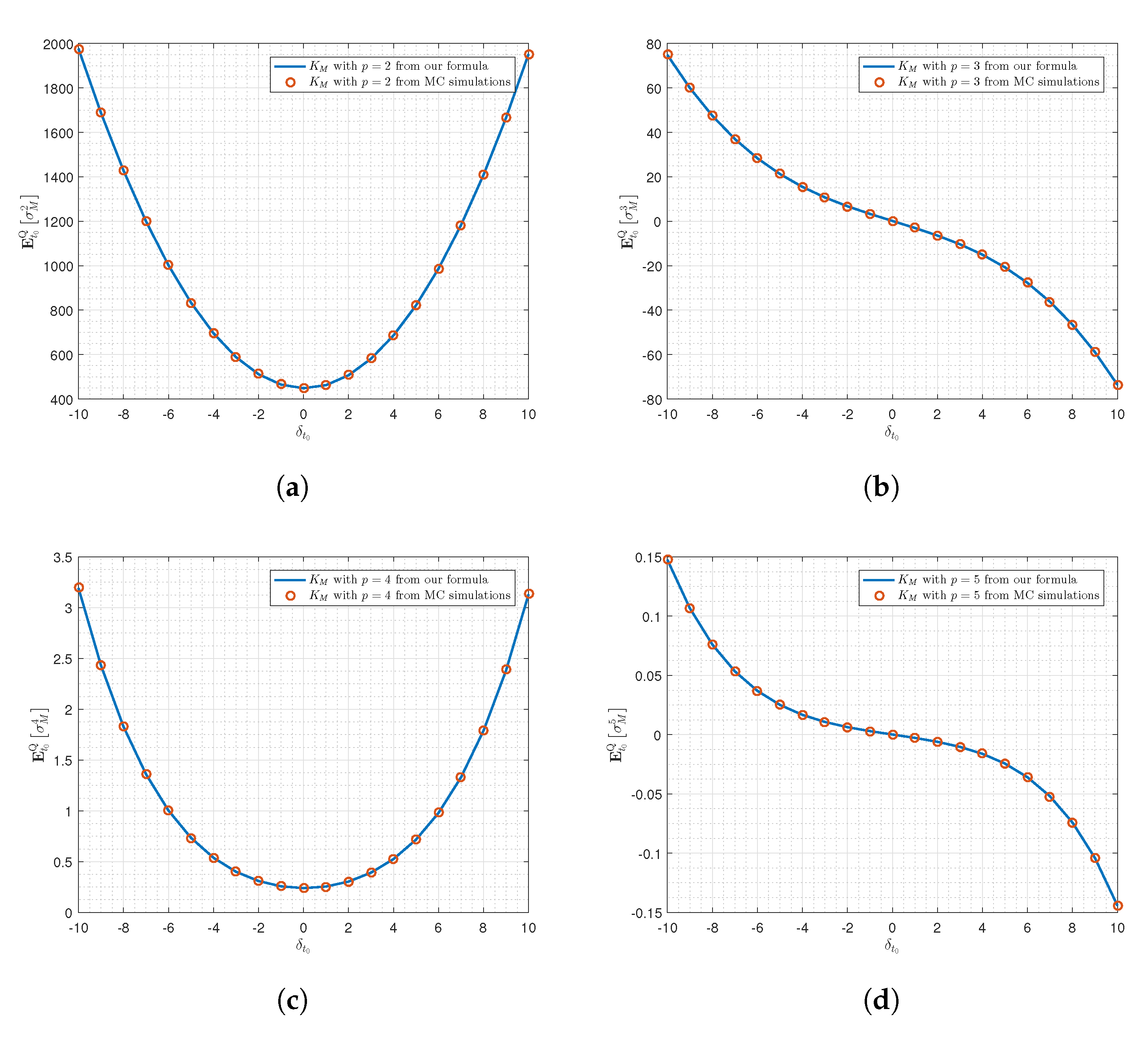
We illustrate only the validations of log-return realized pth-moment swaps given in Section 5.2 when p = 2 , 3 , 4 and 5 via the parameters of the gold spot prices and the prices of gold futures estimated are given in [3]. The parameters are r = 0.05 , σ 1 = 0.212 , κ = 1.187 , α = 0.082 , λ = 0.093 , σ 2 = 0.187 , ρ = 0.845 , N = 253 and T = 1 . To test the efficiency of the pth-moment swaps given in Section 5.2, we compare our obtained results with the MC simulations at various δ t 0 = 10 , 9 , 8 , , 10 . These simulations are constructed with the time step Δ t = 0.0001 and varied with 10,000 sample paths as depicted in Figure 1. Moreover, Figure 1a,c are formed in the symmetric graphs, while Figure 1b,d present the skew-symmetric graphs. In these subfigures, we can clearly see that the solid blue line agrees with the red circle points obtained by the MC simulations.
In this validation, the obtained results of our formula and the MC simulations based on the EM method (34) are run on MATLAB R2021a software, and calculated using a laptop computer configured with: Intel(R) Core(TM) i7-5700HQ, CPU @2.70 GHz, 16.0 GB RAM, Windows 10 and 64-bit Operating System. This work was implemented in MATLAB libraries available in GitHub repositories: https://github.com/TyMathAD/Pricing-Generalized-Swaps accessed on 1 November 2022. In order to measure errors between our formula and the MC simulations, we use the average relative error. This is because it is a good statistical measurement which can be seen in ([55] Table 3) for the model to performance metrics. As a result, the average relative errors of K M with different p = 2 , 3 , 4 and 5 are shown in Table 1. We can see that when path numbers increase, the errors decrease for all p. This means that the results obtained from MC simulations trend toward our closed-form formula. In addition, the consuming times for our closed-form formula depending on p and MC simulations with various numbers of sample paths are also provided in Table 1, which are far more expansive than our formula. Thus, the MC simulations may not represent a good choice in terms of computational time, especially for a large number of sample paths. Therefore, our proposed formula is suggested as highly suitable for practical use.
The main finding of the proposed results appears similar to the results of [3,24] which rely on the closed-form formula for the conditional moments of the log prices E t 0 Q x T n . In this respect, our results displayed in Figure 1a are seen to be equal to the results of variance swaps in [3] in the seam parameters. In addition, our closed-form formula for conditional moments has further beneficial aspects for pricing financial assets whose payoffs can be generated by the conditional moments.
In the case of K M , we refer the readers to Schoutens [53] whose introduces the moment swaps. The K M is a type of derivatives which is depend on realized higher moments of a underlying asset. A well-known case when p = 2 is named the variance swaps which are widely studied in financial mathematics. This contrasts to the cases of p > 2 . Schoutens also shows that the classical hedging by using the variance swaps in the terms of position in log-contracts can be enhanced by using the higher moments, such as, the third moment swaps. In this work, we fulfill the study of Schoutens by showing that the strike price, K M , does not depend on the initial spot price but depends only on the initial convenience yield, δ . In addition, it is in polynomial in δ . This means that we can easily prove that the global critical point with respect to δ for each K is unique by using the first and the second derivative test. In this respect, for the variance swap p = 2 , since the strike price K is a quadratic function in δ , there exists only one global minimizer.

7. Conclusions

This work proposes highly efficient closed-form formulas for pricing generalized swaps, such as actual return-based realized pth-moment swap, log-return realized pth-moment swap, gamma swap, entropy swap and self-quantoed variance swap, based on the affine transformation u in Theorem 1 of the model (3). To calculate u, we rely on the solution of PDE according to the infinitesimal generator for the two-dimensional diffusion process. Under the motivation of the moment-generating function and its derivatives combined with the complete Bell polynomials, the closed-form formulas for the conditional moments and mixed moments of S t , x t , δ t and their products for the model (3) are derived as consequences of Theorem 1, see Theorems 2–4 and Corollaries 2–4.
In addition, some essential properties of closed-form formulas, such as the first and the second conditional moments, conditional variance, conditional central moments, conditional mixed moments and conditional covariance are provided and discussed.

Future Works

Indeed, our general and explicit formulas given in Section 3 and Section 4 can be readily applied to other exotic variance swaps. Since our proposed closed-form formulas are in the form of nth-conditional moments for all n N , our formulas bear further beneficial aspects for pricing financial derivatives whose payoffs can be generated by the moments. Moreover, our proposed method in Section 3 can be applied to find a closed-form formula for conditional moments of each stochastic parameter under the Heston model in addition to three-factor models such as the CIR–Heston hybrid model, which now remain still generally unavailable, as well as in closed forms. Moreover, unlike the model studied by Hilliard and Jorge [56] and Crosby [57], the two-factor model studied herein does not allow for the price to jump by any small magnitudes as addressed in the introduction.

Author Contributions

Conceptualization, A.D., R.B., U.R. and P.S.; methodology, A.D. and P.S.; software, A.D. and P.S.; validation, A.D., R.B., U.R. and P.S.; formal analysis, A.D., R.B., U.R. and P.S.; investigation, A.D., R.B., U.R. and P.S.; writing—original draft preparation, A.D. and P.S.; writing—review and editing, R.B. and U.R.; visualization, A.D. and P.S.; supervision, R.B. and U.R.; funding acquisition, R.B. and U.R. All authors have read and agreed to the published version of the manuscript.

Funding

This research received no external funding.

Institutional Review Board Statement

Not applicable.

Informed Consent Statement

Not applicable.

Data Availability Statement

Not applicable.

Acknowledgments

We are grateful for valuable comments and suggestions from the anonymous referees that have improved the quality of this paper. This research project is supported by Second Century Fund (C2F), Chulalongkorn University.

Conflicts of Interest

The authors declare no conflict of interest.

Abbreviations

The following abbreviations are used in this manuscript:
CIRCox–Ingersoll–Ross
EMEuler–Maruyama
MCMonte Carlo
OUOrnstein–Uhlenbeck
PDEPartial differential equation
SDEStochastic differential equation

References

  1. Chumpong, K.; Mekchay, K.; Rujivan, S.; Thamrongrat, N. Simple Analytical Formulas for Pricing and Hedging Moment Swaps. Thai J. Math. 2022, 20, 693–713. [Google Scholar]
  2. Chumpong, K.; Tanadkithirun, R.; Tantiwattanapaibul, C. Simple closed-form formulas for conditional moments of inhomogeneous nonlinear drift constant elasticity of variance process. Symmetry 2022, 14, 1345. [Google Scholar] [CrossRef]
  3. Rujivan, S. Analytically pricing variance swaps in commodity derivative markets under stochastic convenience yields. Commun. Math. Sci. 2021, 19, 111–146. [Google Scholar] [CrossRef]
  4. Swishchuk, A.V. Variance and volatility swaps in energy markets. J. Energy Mark. 2013, 6, 33–49. [Google Scholar] [CrossRef]
  5. Zhu, S.P.; Lian, G.H. A closed-form exact solution for pricing variance swaps with stochastic volatility. Math. Financ. An Int. J. Math. Stat. Financ. Econ. 2011, 21, 233–256. [Google Scholar]
  6. Schwartz, E.S. The stochastic behavior of commodity prices: Implications for valuation and hedging. J. Financ. 1997, 52, 923–973. [Google Scholar] [CrossRef]
  7. Uhlenbeck, G.E.; Ornstein, L.S. On the theory of the Brownian motion. Phys. Rev. 1930, 36, 823. [Google Scholar] [CrossRef]
  8. Algieri, B. Price volatility, speculation and excessive speculation in commodity markets: Sheep or shepherd behaviour? ZEF-Discuss. Pap. Dev. Policy 2012, 166, 37. [Google Scholar] [CrossRef]
  9. Algieri, B. Conditional price volatility, speculation, and excessive speculation in commodity markets: Sheep or shepherd behaviour? Int. Rev. Appl. Econ. 2016, 30, 210–237. [Google Scholar] [CrossRef]
  10. Lu, X.; Zhu, S.P.; Yan, D. Nonlinear PDE model for European options with transaction costs under Heston stochastic volatility. Commun. Nonlinear Sci. Numer. Simul. 2021, 103, 105986. [Google Scholar] [CrossRef]
  11. Zhu, S.P.; Lian, G.H. On the valuation of variance swaps with stochastic volatility. Appl. Math. Comput. 2012, 219, 1654–1669. [Google Scholar] [CrossRef]
  12. Zhu, S.P.; Lian, G.H. Analytically pricing volatility swaps under stochastic volatility. J. Comput. Appl. Math. 2015, 288, 332–340. [Google Scholar] [CrossRef]
  13. Zhu, S.P.; Lian, G.H. On the convexity correction approximation in pricing volatility swaps and VIX futures. New Math. Nat. Comput. 2018, 14, 383–401. [Google Scholar] [CrossRef]
  14. Lee, Y.; Kim, Y.; Lee, J. Pricing Various Types of Power Options under Stochastic Volatility. Symmetry 2020, 12, 1911. [Google Scholar] [CrossRef]
  15. Chunhawiksit, C.; Rujivan, S. Pricing discretely-sampled variance swaps on commodities. Thai J. Math. 2016, 14, 711–724. [Google Scholar]
  16. Weraprasertsakun, A.; Rujivan, S. A closed-form formula for pricing variance swaps on commodities. Vietnam. J. Math. 2017, 45, 255–264. [Google Scholar] [CrossRef]
  17. Chumpong, K.; Mekchay, K.; Thamrongrat, N. Analytical formulas for pricing discretely-sampled skewness and kurtosis swaps based on Schwartz’s one-factor model. Songklanakarin J. Sci. Technol. 2020, 43, 465–470. [Google Scholar]
  18. Chumpong, K.; Mekchay, K.; Rujivan, S. A simple closed-form formula for the conditional moments of the Ornstein–Uhlenbeck process. Songklanakarin J. Sci. Technol. 2020, 42, 836–845. [Google Scholar]
  19. Duffie, D.; Pan, J.; Singleton, K. Transform analysis and asset pricing for affine jump-diffusions. Econometrica 2000, 68, 1343–1376. [Google Scholar] [CrossRef] [Green Version]
  20. Karatzas, I.; Shreve, S. Brownian Motion and Stochastic Calculus; Springer Science & Business Media: Berlin, Germany, 2012; Volume 113. [Google Scholar]
  21. Blanco, C.; Soronow, D. Mean reverting processes-energy price processes used for derivatives pricing & risk management. Commod. Now 2001, 5, 68–72. [Google Scholar]
  22. Issaranusorn, N.; Rujivan, S.; Mekchay, K. Stochastic model for gold prices ans its application for noarbitrage pricing. J. Nonlinear Anal. Optim. Theory Appl. 2011, 2, 11–17. [Google Scholar]
  23. Allaire, G.; Kaber, S.M.; Trabelsi, K.; Allaire, G. Numerical Linear Algebra; Springer: Berlin, Germany, 2008; Volume 55. [Google Scholar]
  24. Kim, S.W.; Kim, J.H. Pricing generalized variance swaps under the Heston model with stochastic interest rates. Math. Comput. Simul. 2020, 168, 1–27. [Google Scholar] [CrossRef]
  25. Duffie, D.; Filipović, D.; Schachermayer, W. Affine processes and applications in finance. Ann. Appl. Probab. 2003, 13, 984–1053. [Google Scholar] [CrossRef]
  26. Filipović, D.; Larsson, M. Polynomial diffusions and applications in finance. Financ. Stoch. 2016, 20, 931–972. [Google Scholar] [CrossRef] [Green Version]
  27. Filipović, D. Term-Structure Models: A Graduate Course; Springer Science & Business Media: Berlin, Germany, 2009. [Google Scholar]
  28. Filipović, D.; Mayerhofer, E. Affine diffusion processes: Theory and applications. Adv. Financ. Model. 2009, 8, 1–40. [Google Scholar] [CrossRef] [Green Version]
  29. Johnson, W.P. The curious history of Faà di Bruno’s formula. Am. Math. Mon. 2002, 109, 217–234. [Google Scholar]
  30. Olver, P.J. Applications of Lie Groups to Differential Equations; Springer Science & Business Media: Berlin, Germany, 2000; Volume 107. [Google Scholar]
  31. Laohakosol, V.; Meesa, R.; Sutthimat, P. Closed-form solutions of general second order linear recurrences and applications. Discret. Math. 2023, 346, 113206. [Google Scholar] [CrossRef]
  32. Forman, J.L.; Sørensen, M. The Pearson diffusions: A class of statistically tractable diffusion processes. Scand. J. Stat. 2008, 35, 438–465. [Google Scholar] [CrossRef]
  33. Sutthimat, P.; Mekchay, K. Closed-form formulas for conditional moments of inhomogeneous Pearson diffusion processes. Commun. Nonlinear Sci. Numer. Simul. 2022, 106, 106095. [Google Scholar] [CrossRef]
  34. Han, Y.; Zhao, L. A closed-form pricing formula for variance swaps under MRG–Vasicek model. Comput. Appl. Math. 2019, 38, 1–17. [Google Scholar] [CrossRef]
  35. He, X.J.; Zhu, S.P. A series-form solution for pricing variance and volatility swaps with stochastic volatility and stochastic interest rate. Comput. Math. Appl. 2018, 76, 2223–2234. [Google Scholar] [CrossRef]
  36. Zheng, W.; Kwok, Y.K. Closed form pricing formulas for discretely sampled generalized variance swaps. Math. Financ. 2014, 24, 855–881. [Google Scholar] [CrossRef]
  37. Nonsoong, P.; Mekchay, K.; Rujivan, S. An analytical option pricing formula for mean-reverting asset with time-dependent parameter. ANZIAM J. 2021, 63, 178–202. [Google Scholar]
  38. Boonklurb, R.; Duangpan, A.; Rakwongwan, U.; Sutthimat, P. A Novel Analytical Formula for the Discounted Moments of the ECIR Process and Interest Rate Swaps Pricing. Fractal Fract. 2022, 6, 58. [Google Scholar] [CrossRef]
  39. Nualsri, F.; Mekchay, K. Analytically Pricing Formula for Contingent Claim with Polynomial Payoff under ECIR Process. Symmetry 2022, 14, 933. [Google Scholar] [CrossRef]
  40. Sutthimat, P.; Mekchay, K.; Rujivan, S. Explicit formula for conditional expectations of product of polynomial and exponential function of affine transform of extended Cox–Ingersoll–Ross process. In Proceedings of the Journal of Physics: Conference Series; IOP Publishing: Bristol, UK, 2018; Volume 1132, p. 012083. [Google Scholar]
  41. Sutthimat, P.; Mekchay, K.; Rujivan, S. Closed-form formula for conditional moments of generalized nonlinear drift CEV process. Appl. Math. Comput. 2022, 428, 127213. [Google Scholar] [CrossRef]
  42. Sutthimat, P.; Rujivan, S.; Mekchay, K.; Rakwongwan, U. Analytical formula for conditional expectations of path-dependent product of polynomial and exponential functions of extended Cox–Ingersoll–Ross process. Res. Math. Sci. 2022, 9, 1–17. [Google Scholar] [CrossRef]
  43. Benth, F.E. Pricing of commodity and energy derivatives for polynomial processes. Mathematics 2021, 9, 124. [Google Scholar] [CrossRef]
  44. Duangpan, A.; Boonklurb, R.; Chumpong, K.; Sutthimat, P. Analytical Formulas for Conditional Mixed Moments of Generalized Stochastic Correlation Process. Symmetry 2022, 14, 897. [Google Scholar] [CrossRef]
  45. Aronow, P.M.; Miller, B.T. Foundations of Agnostic Statistics; Cambridge University Press: Cambridge, UK, 2019. [Google Scholar]
  46. Sørensen, M. Prediction-based estimating functions. Econom. J. 2000, 3, 123–147. [Google Scholar] [CrossRef]
  47. Leonenko, N.N.; Šuvak, N. Statistical inference for reciprocal gamma diffusion process. J. Stat. Plan. Inference 2010, 140, 30–51. [Google Scholar] [CrossRef]
  48. Leonenko, N.N.; Šuvak, N. Statistical inference for Student diffusion process. Stoch. Anal. Appl. 2010, 28, 972–1002. [Google Scholar] [CrossRef]
  49. Avram, F.; Leonenko, N.N.; Šuvak, N. Parameter estimation for Fisher–Snedecor diffusion. Statistics 2011, 45, 27–42. [Google Scholar] [CrossRef]
  50. Gouriéroux, C.; Valéry, P. Estimation of a Jacobi Process; Technical Report; Université de Montréal: Montreal, QC, Canada, 2004; Volume 116. [Google Scholar]
  51. Forman, J.L. Least Squares Estimation for Autocorrelation Parameters with Applications to Sums of Ornstein–Uhlenbeck Type of Processes; Department of Applied Mathematics and Statistics, University of Copenhagen: Copenhagen, Denmark, 2005. [Google Scholar]
  52. Prunglerdbuathong, P.; Mekchay, K.; Rujivan, S. Parameter estimation of one-dimensional Ito processes by LTDRM. Thai J. Math. 2015, 13, 123–136. [Google Scholar]
  53. Schoutens, W. Moment swaps. Quant. Financ. 2005, 5, 525–530. [Google Scholar] [CrossRef]
  54. Crosby, J. Exact pricing of discretely-sampled variance derivatives. J. Bus. Manag. Appl. Econ. 2013. [Google Scholar]
  55. Bolboacă, S.D.; Jäntschi, L. Sensitivity, specificity, and accuracy of predictive models on phenols toxicity. J. Comput. Sci. 2014, 5, 345–350. [Google Scholar] [CrossRef]
  56. Hilliard, J.E.; Reis, J.A. Jump processes in commodity futures prices and options pricing. Am. J. Agric. Econ. 1999, 81, 273–286. [Google Scholar] [CrossRef]
  57. Crosby, J. A multi-factor jump-diffusion model for commodities. Quant. Financ. 2008, 8, 181–200. [Google Scholar] [CrossRef]
Figure 1. The validation testings of log-return realized pth-moment swaps for various values p. (a) K M with p = 2 . (b) K M with p = 3 . (c) K M with p = 4 . (d) K M with p = 5 .
Symmetry 14 02385 g001
Table 1. Average relative errors and run times of log-return realized pth-moment swaps K M compared with our formula using MC simulations.
Path NumbersAverage Relative Errors of K M Run Time of MC Simulation
p = 2 p = 3 p = 4 p = 5
5000 2.065 × 10 3 1.514 × 10 2 3.811 × 10 3 2.665 × 10 2 1.204827 s
10,000 1.368 × 10 3 5.737 × 10 3 2.911 × 10 3 6.011 × 10 3 2.321888 s
20,000 8.535 × 10 4 2.022 × 10 3 1.843 × 10 3 1.636 × 10 3 4.663894 s
40,000 6.482 × 10 4 8.195 × 10 4 9.244 × 10 4 3.651 × 10 4 8.349923 s
80,000 4.047 × 10 4 6.426 × 10 4 7.107 × 10 4 1.349 × 10 4 16.42857 s
Run time of our formula0.003944 s0.006184 s0.008273 s0.010671 s
Publisher’s Note: MDPI stays neutral with regard to jurisdictional claims in published maps and institutional affiliations.

