Article

Radar-Jamming Classification in the Event of Insufficient Samples Using Transfer Learning

1
The Department of Remote Sensing Science and Technology, School of Electronic Engineering, Xidian University, Xi’an 710071, China
2
The Key Laboratory of High-Speed Circuit Design and EMC Ministry of Education, The School of Electronic Engineering, Xidian University, Xi’an 710071, China
*
Author to whom correspondence should be addressed.
Symmetry 2022, 14(11), 2318; https://doi.org/10.3390/sym14112318
Submission received: 9 September 2022 / Revised: 25 October 2022 / Accepted: 1 November 2022 / Published: 4 November 2022

Abstract

:
Radar has played an irreplaceable role in modern warfare. A variety of radar-jamming methods have been applied in recent years, which makes the electromagnetic environment more complex. The classification of radar jamming is critical for electronic counter-countermeasures (ECCM). In the field of signal classification, machine learning-based methods take great effort to find proper features as well as classifiers, and deep learning-based methods depend on large training datasets. For the above reasons, an efficient transfer learning-based method is proposed in this paper. Firstly, one-dimensional radar signals were transformed into time–frequency images (TFIs) using linear and bilinear time–frequency analysis, which is inspired by symmetry theory. Secondly, pretrained AlexNet and SqueezeNet networks were modified to classify the processed TFIs. Finally, performance of this method was evaluated and compared using a simulated data set with nine types of radar-jamming signals. The results demonstrate that our proposed classification method performs well in accuracy and efficiency at a 1% training ratio, which is practical for anti-jamming.

1. Introduction

Radar jamming is a long-standing topic in modern electronic warfare [1,2,3]. With the development of digital radio frequency memory (DRFM) technology, the types of radar-jamming signals become more diverse. Existing anti-jamming measures are designed for specific jamming types [4]. Therefore, in order to improve the anti-jamming ability of one’s radar system, the primary effort is to distinguish the different jamming signals of the enemy radar.
Jamming radar is intended to destroy and disturb the radar’s detection of the target. Radar jamming can be divided into suppression jamming and deception jamming [5]. Suppression jamming mainly destroys the ability of radar to find targets and measure target parameters. Suppression jamming reduces the signal-to-noise ratio (SNR) [6] when radar detects targets. When the false alarm probability is determined, the radar detection ability is positively related to the SNR of the signal. According to the center frequency and bandwidth of the jamming signal and the relevance to the center frequency and bandwidth of the radar signal, suppression jamming can be divided into spot jamming (SJ), blocking jamming (BJ), and linear sweeping jamming (LSJ) [7,8,9]. Deception jamming provides false targets or target information to enemy radar [10], triggering false alarms. Compared with suppression jamming, deception jamming is more complicated. Three typical types of deception jamming are investigated in this paper: dense false target jamming (DFTJ) [5], interrupted-sampling repeater jamming (ISRJ) [11,12] and smart noise jamming (SNJ) [13,14]. Of course, there are other types of jamming that deserve study in future work.
The existing classification methods for radar-jamming signals include machine learning-based methods and deep learning-based methods. Although the deep learning method was born relatively late, it shows an extraordinary ability in multi-class classification [15,16]. Unlike traditional machine learning methods, a convolutional neural network (CNN) can directly input high-dimensional data [17]. In order to load training sets into a CNN, researchers mathematically transform 1D time-domain signals into 2D time–frequency images (TFIs) [18]. Generally, time–frequency analysis methods include short-time Fourier transform (STFT), Wigner–Ville distribution (WVD) [19], and smoothed pseudo-WVD (SPWVD) [20]. For example, Shao et al. [21] and Lv et al. [22] used STFT and a self-built CNN to classify radar-jamming signals. Because STFT cannot achieve high resolution in both the time and frequency domains simultaneously, their works relied on information fusion methods. Shao et al. fused the 1D and 2D signal information [21]. Lv et al. fused the real parts, imaginary parts, modulus, and phase of a radar-jamming signal [22]. Inspired by symmetry theory, our solution turned from linear time–frequency analysis (STFT) to bilinear time–frequency analysis (WVD, SPWVD). The resolution of a signal’s WVD and SPWVD is much higher than its STFT, so there is no need to fuse information when using WVD or SPWVD. For example, Wang et al. used WVD for the automatic recognition of radar waveforms [23]. WVD and SPWVD have higher resolution than STFT, making them more suitable for dealing with complicated classification tasks. A well-performed CNN model greatly depends on a well-designed network structure and massive data. In the field of signal classification, many researchers have established their own CNN. However, these self-built structures have insufficient performance due to their simple network structure and insufficient data. These networks still have a lot of room for improvement in terms of recognition accuracy. Transfer learning is a technique for fine-tuning a pretrained network trained on a large, labeled dataset in order to apply it to small samples [24]. Therefore, transfer learning is more applicable to classification when the data are scarce and building neural networks is difficult. For example, Li et al. used a pretrained CNN to identify navigation signal interference types [25]. It shows that transfer learning can effectively speed up the convergence of the CNN without compromising the performance of the model.
Our contributions are as follows: (1) With the help of time–frequency analysis, 1D jamming signals were converted into 2D TFIs, which facilitated the subsequent automatic feature extraction; (2) Using the transfer learning method, the classification of jamming was realized. The time and workload of redesigning and training new networks was saved by modifying pretrained networks; (3) While ensuring accuracy, the application of lightweight SqueezeNet greatly reduced the demand for computing power and memory usage. Therefore, our method has the potential to be deployed on embedded devices.
In this paper, a classification method based on transfer learning and SPWVD is proposed to reduce manpower and achieve high recognition accuracy in case of small sample size. The rest of this paper is organized as follows. Firstly, Section 2 introduces the cardinal principle of the algorithm in this paper. Secondly, the experimental results are presented and analyzed in Section 3. Finally, Section 4 concludes this work and discusses future work.

2. Materials and Methods

The flowchart of transfer learning-based methods for active radar-jamming classification is shown in Figure 1. Figure 1 shows the important parts of our paper and reveals the connections among them. Through data preparation, network construction, and multiple simulation experiments, a final classification method was found. This section mainly introduces the elementary methods of our work.

2.1. Radar-Jamming Signals

In this work, we needed to construct a data set of active jamming signals. The mathematical formulas of the jamming signals are given below, including one signal without jamming, three suppression jamming signals, three deception jamming signals, and two composite -jamming signals. The default is that they are pulse signals based on linear frequency modulation (LFM). The waveform of an LFM radar pulse signal in the time domain can be expressed as [26]:
S ( t ) = A r e c t ( t T ) exp [ j 2 π ( f 0 t + 1 2 B T t 2 ) ]
where A is the amplitude, f 0 is the center frequency, T is the pulse duration, B is the bandwidth, and rectangle function r e c t ( t T ) is defined as:
r e c t ( t T ) = { 1 T 2 t T 2 0 otherwise

2.1.1. Interrupted Sampling Repeater Jamming (ISRJ)

In order to realize this jamming, the jammer retransmits the intercepted radar signal multiple times. Its time domain model can be expressed as:
J I S R J ( t ) = m = 1 M n = 0 N r e c t ( t ( n M + n + m ) T W T W ) S ( t m T w )
where N is the number of slices, T w is the time duration of each slice, and M refers to how many times a slice is retransmitted.

2.1.2. Dense False Target Jamming (DFTJ)

The jammer intercepts a radar signal by delaying, stacking, and forwarding the signal many times. Jammers cause the radar to form multiple false targets at different distances. Its time domain model can be expressed as:
J D F T J ( t ) = m = 1 M A m S ( t t 0 τ m )
where A m is the modulation amplitude, t 0 is the time delay of the real target echo, and τ m is the time delay after m times’ retransmission.

2.1.3. Smart Noise Jamming (SNJ)

Smart noise jamming has the effect of noise jamming and spoofing. In this paper, interrupted sampling repeater jamming was multiplied by white Gaussian noise to make a smart noise interference. Its time domain model can be expressed as:
J S N J ( t ) = n ( t ) J I S R J ( t )
where n ( t ) refers to white Gaussian noise with zero mean and variance σ 2 .

2.1.4. Blocking Jamming (BJ) and Spot Jamming (SJ)

These two are suppression interferences. They both produce a wide interference bandwidth. However, the jamming power of spot jamming is only strong in the operating frequency of the radar. Blocking jamming can cover a wider bandwidth.
{ f j f s Δ f j 1 ( 2 ~ 5 ) Δ f r   Δ f j 2 5 Δ f r
where Δ f r is the bandwidth of the radar receiver, f s is the center frequency of the radar receiver, f j is the center frequency of jamming signal, Δ f j 1 is the bandwidth of spot jamming, and Δ f j 2 is the bandwidth of blocking jamming. These formulas define themselves mainly based on the frequency range.

2.1.5. Linear Sweep Jamming (LSJ):

LSJ as adopted in this paper satisfies the following conditions:
{ f j = f s ± k t   t [ 0 , T j ] Δ f j ( 2 ~ 5 ) Δ f r
where k is the chirp rate, k = B T . Δ f r is the bandwidth of the radar receiver, f s is the center frequency of the radar receiver, f j is the center frequency of the jamming signal, and f j is periodic function.
With these mathematical expressions, a simulation database of radar-jamming signals was constructed.

2.2. Joint Time–Frequency Analysis

In our experiments, STFT, WVD, and SPWVD were used to transform 1D radar-jamming signals into TFIs.

2.2.1. Short-Time Fourier Transform (STFT)

The short-time Fourier transform (STFT) is the mainstream approach to analyzing a signal with time-varying frequency [27]. This method divides the time-domain signal into multiple segments, and then takes a Fourier transform of each segment. φ ( t ) is the window function of the signal segment. For a continuous signal x ( t ) , the STFT operation is defined as [28]:
STFT x ( t , ω ) = + x ( τ ) φ ( τ t ) e j ω τ d τ
where τ is center position of φ ( τ t ) and represents the conjugate operation. The other operations are the same as for Fourier transform. STFT is a Fourier transform of the original signal in a small duration range. According to the uncertainty principle, STFT is unable to obtain a high resolution in the time domain and frequency domain simultaneously.

2.2.2. Wigner–Ville Distribution (WVD)

The Wigner–Ville distribution was proposed by Ville in 1948 [29]. The WVD is defined as a Fourier transform of the instantaneous correlation function of the signal [30]. For a continuous signal x ( t ) , the Wigner–Ville distribution is defined as:
WVD x ( t , f ) = x ( t + τ 2 ) x ( t τ 2 ) e j 2 π f τ d τ  
Generally speaking, WVD does not involve a window function, which avoids the mutual restriction between time domain resolution and frequency domain resolution. For a single-component LFM signal, WVD has good energy concentration. However, when analyzing multi-component signals, WVD is disturbed by cross-terms.

2.2.3. Smoothed Pseudo-WVD (SPWVD)

Researchers have proposed many improved methods to suppress the influence of cross-terms. In order to overcome the impact of cross-terms, Barbarossa proposed a pseudo-Wigner–Ville distribution (PWVD) by adding a smoothing window in the time domain. In 2003, Zhao Jun et al. cited Barbarossa’s work and employed smooth pseudo-Wigner–Ville distribution (SPWVD) on the basis of PWVD to estimate the parameter of frequency-hopping signals [29]. SPWVD can filter interference terms with low-pass windows. It uses independent windows to smooth time and frequency:
SPWVD x g , H ( t , f ) = g ( t ) H ( f ) x ( t + τ 2 ) x ( t τ 2 ) e j 2 π f τ d τ
By adding smooth windows, the cross-term interference is substantially eliminated in SPWVD.

2.3. Pretrained Network Modification

Transfer learning takes pretrained networks as the starting point for new tasks. Fine-tuning the pretrained networks is usually much faster and easier than training networks using random initialization weights from scratch. Especially when there are small training samples, transfer learning can quickly transfer learned features onto new tasks. In this paper, we used two pretrained networks: a pretrained AlexNet and a pretrained SqueezeNet. AlexNet, employing an 8-layer CNN, won the ImageNet Large-Scale Visual Recognition Challenge 2012 by a phenomenally large margin [31]. Since then, many classic image classification models based on deep convolutional neural networks have been developed. After that, Forrest et al. proposed the SqueezeNet, which achieved AlexNet-level accuracy with 50× fewer parameters [32]. This facilitated CNNs applications on lightweight hardware devices.
AlexNet has been trained on more than one million images from datasets. The pretrained network can classify 1000 object categories, such as keyboard, mouse, pencil, and many animals. Therefore, AlexNet has learned rich feature representations for a wide range of images. SqueezeNet can also achieve the same classification accuracy. The input image size for AlexNet and SqueezeNet is 227 × 227 × 3. There are several typical layers in these nets, as detailed below.

2.3.1. Convolutional Layers

The purpose of a convolutional layer is to use a convolution kernel to scan images line by line and finally extract the features of the image. Specifically, the input of a convolutional layer is the 3D matrix X with a size of m1 × m2 × n. The convolutional layer itself is a variable matrix in which the parameters change. After multiplication, addition, and offset operations, new results are obtained and input into the next layer. The results are feature maps.

2.3.2. Dropout Layers

When there are more parameters and less training data, the nets can perfectly fit training data but may not perform well on the verification data. The main function of the dropout layer is to prevent over-fitting. A high degree of fitting will lead to poor adaptability of the radar-jamming classification model. So, some results need to be discarded.

2.3.3. Fully Connected Layers

Each node of the fully connected layer is connected with all nodes of the previous layer. It acts as a classifier, mapping the features to each class label and outputting the probability matrix of each sample. Because the number of the fully connected layer’s parameters is huge, The fully connected layer is generally used for the output layer.
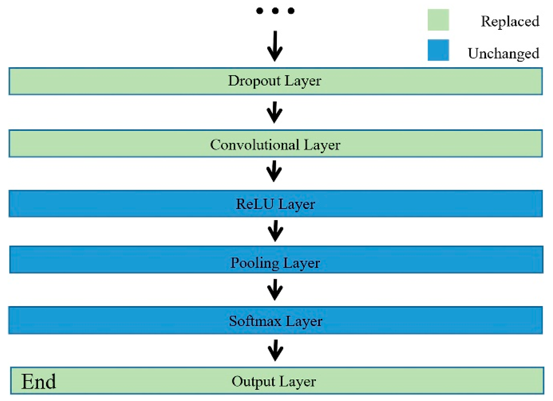
Based on this knowledge of CNNs, we modified some pretrained nets. For instance, Figure 2 shows the modification to the last six layers of the pretrained SqueezeNet. The green layers are the new layers after replacement.

3. Results

In this section, a data set of 1D active jamming signals was first constructed. Then, different time–frequency analysis techniques were used to transform 1D radar signals, and the generated TFIs are compared. Thirdly, the pretrained networks were modified to realize the subsequent classification. Finally, the performances of different methods are compared, and a high-accuracy method is found. All experiments were designed and performed on a desktop computer with the following hardware configurations:
Intel i7-100700F/16GB RAM/512GB SSD/NVIDIA GeForce GTX 1660 SUPER.

3.1. Simulation of 1D Radar-Jamming Signals

A 1D simulation dataset of nine types of signals was constructed, including one signal without jamming, three deception jamming signals (ISRJ, DFTJ, and SNJ), three suppression jamming signals (BJ, SJ, and LSJ), and two composite jamming signals (DFTJ + SNJ, ISRJ + LSJ). In the dataset, each type of active jamming signal had 1000 samples. Each sample contained a true target echo with random location variation and different jamming. Detailed parameters are shown in Table 1.
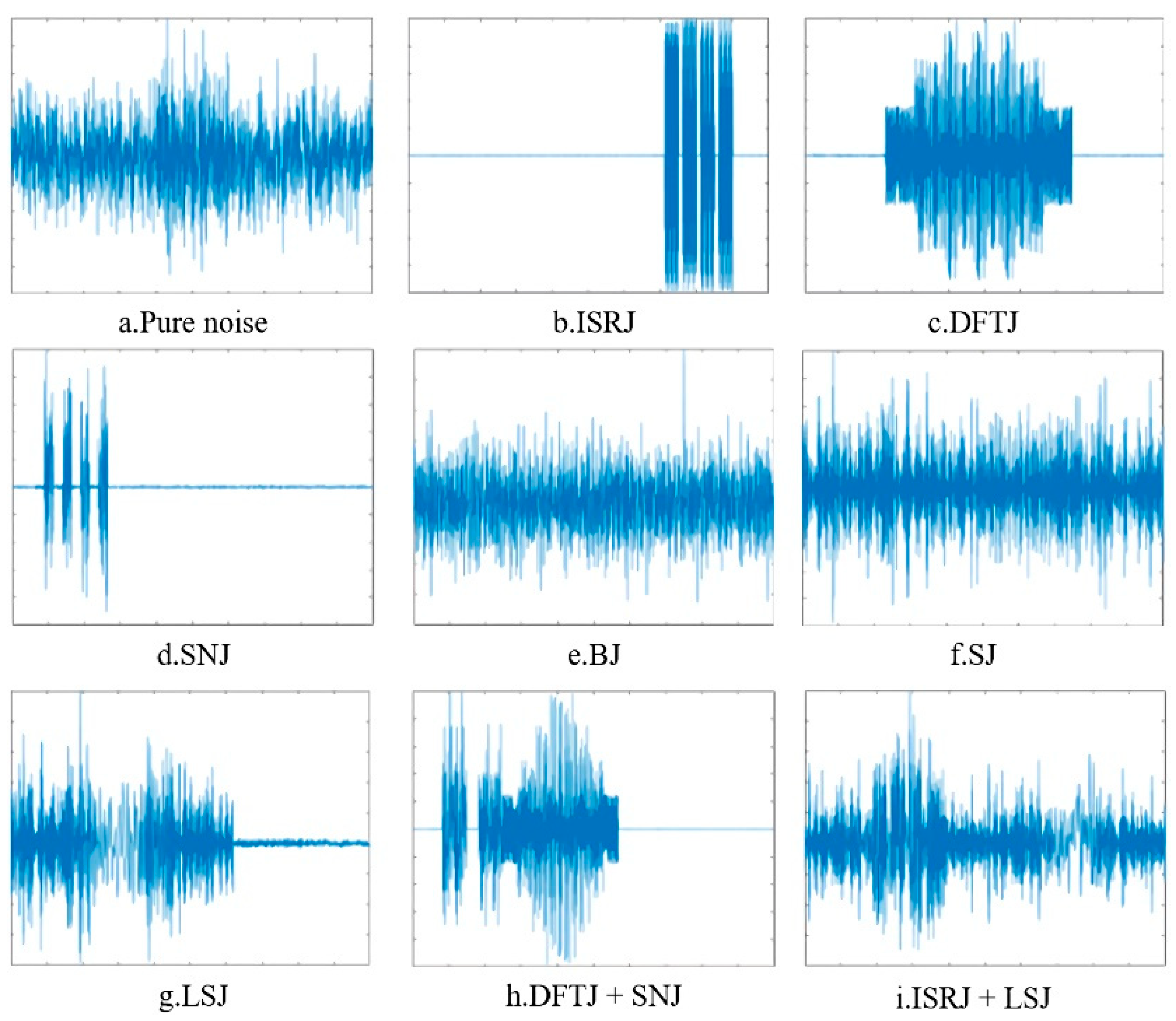
The LFM waveform (B = 10 MHz, T = 20 μs) was used as the radar transmission signal, and each 1D signal’s width was 100 μs with a sampling rate of 20 MHz/s. Therefore, each sample had 4000 real-valued elements, 2000 for real parts and 2000 for imaginary parts, respectively. Figure 3 shows the real-part waveforms with normalized amplitude of each type of active jamming signal.

3.2. Jamming TFI Processing

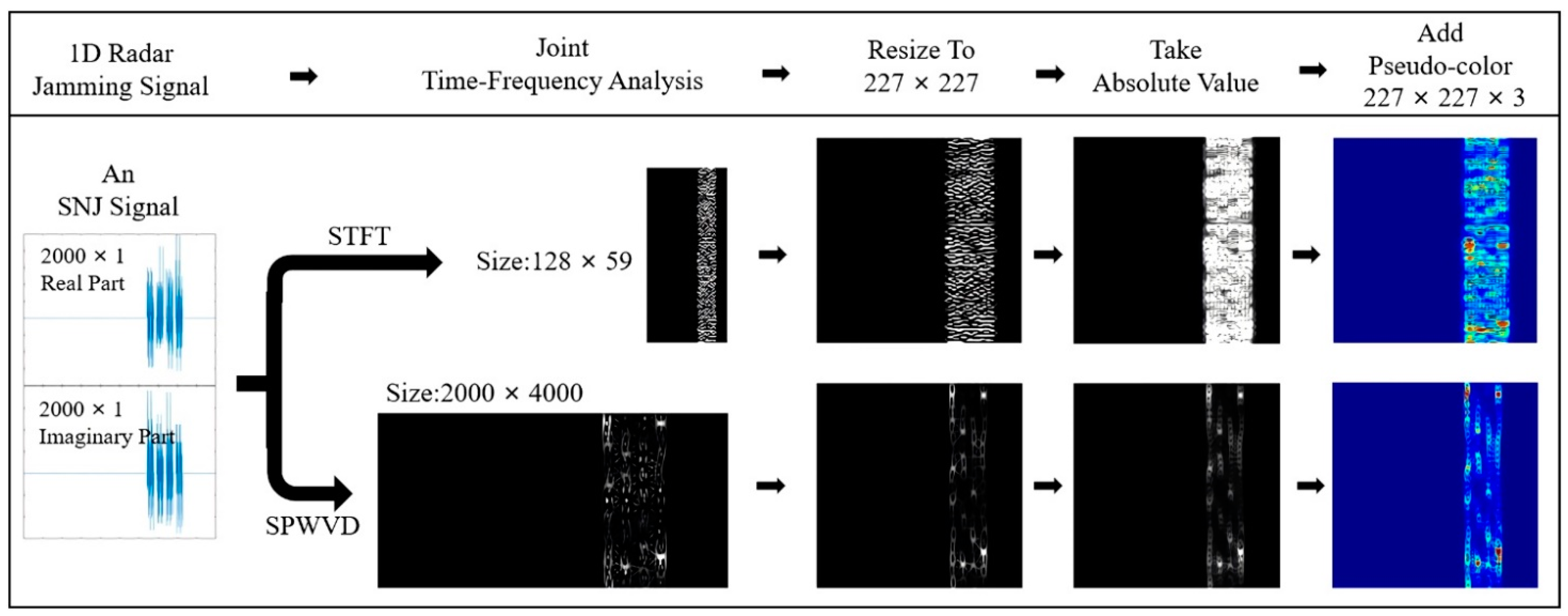
STFT, WVD, and SPVWD represent time–frequency views of 1D radar-jamming data. STFT, WVD, and SPWVD were calculated for each signal. These results were resized, and pseudo-color was added. During image resizing, new pixel values were obtained using the weighted average of pixels in the nearest neighbors, and the recognizability of the image was increased by mapping the image to a pseudo-color space. It is worth mentioning that we took complex signals as the object of time–frequency analysis. The operation of taking absolute value was performed in order to eliminate the influence of complex numbers that come from time–frequency analysis. Figure 4 shows the processing steps for an SNJ’s STFT and SPWVD.
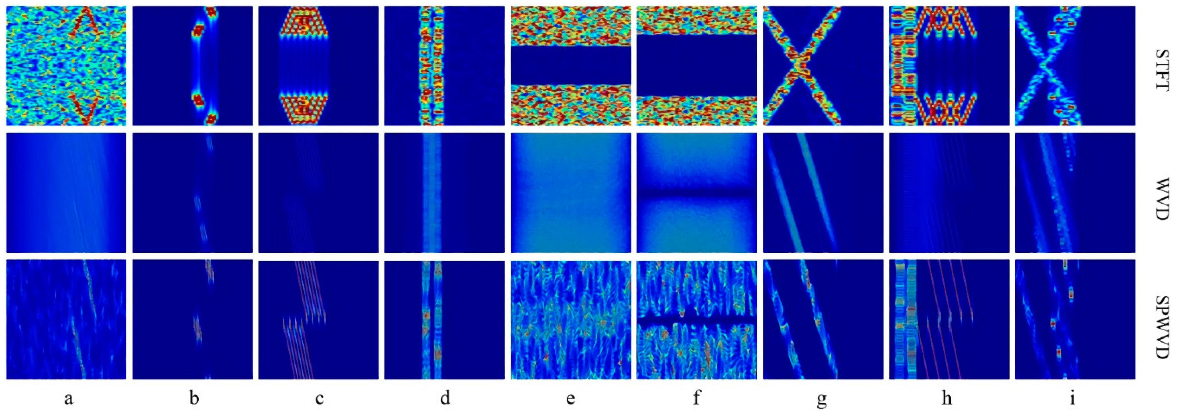
For each radar-jamming signal, three 227 × 227 × 3 images (STFT, WVD, and SPVWD TFIs) were saved. These TFIs were taken as the CNN’s input. Figure 5 shows these different TFIs. These images provided a representation of the input data, making it easier for the classification algorithm to distinguish different categories. It is noteworthy that the superposition mode of composite signals can be easily perceived in SPWVD TFIs, as shown in Figure 5h,i.

3.3. Modification of Deep Learning Networks

TFIs of radar-jamming signals were adjusted to 227 × 227 × 3, so the input layer of the pretrained networks did not need to change. The last few layers affected whether the net was a suitable classifier. Taking the pretrained SqueezeNet as an example, we changed these layers. The altering of the last six layers of the modified net can be found in Table 2. The modified net was suitable for nine kinds of jamming classification. The modification method of the pretrained AlexNet was similar.

3.4. Comparisons

3.4.1. The More-Efficient SqueezeNet

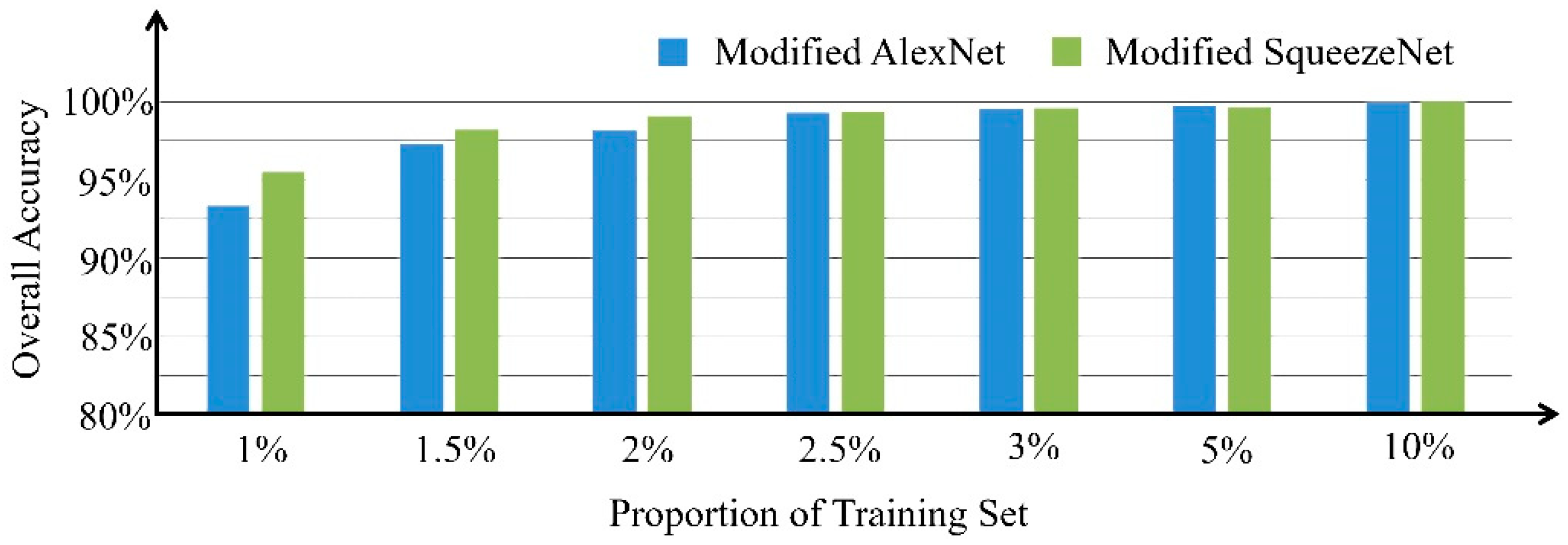
Two pretrained networks, AlexNet and SqueezeNet, were modified and trained using signals’ WVD TFIs. After only five training epochs, good classification accuracy was achieved by both networks, as shown in Figure 6. The modified networks based on AlexNet and SqueezeNet showed little difference in overall accuracy (OA), while the latter had a faster convergence rate. When the training ratio was extremely small, the modified AlexNet failed to achieve the same high OA as the modified SqueezeNet after five epochs’ training.
In addition to accuracy, efficiency is also an important performance index in a practical setting. Although both of the aforementioned networks can obtain good classification accuracy in a short training time, the memory usage of the modified SqueezeNet was only 1% of that of the modified AlexNet, as shown in Figure 7. The memory usage is local storage space occupied by the generated prediction model.
To sum up, the modified SqueezeNet was more efficient than the modified AlexNet in terms of convergence speed and memory usage.

3.4.2. Comparison between STFT and WVD

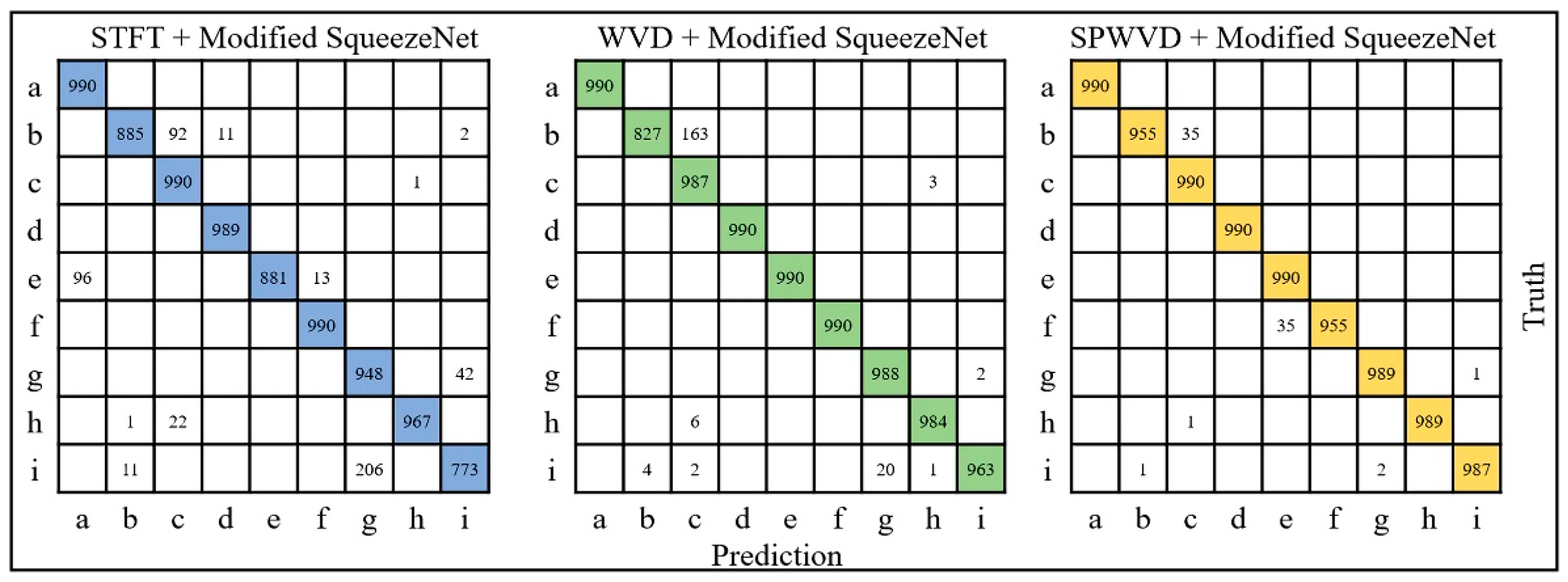
We compared using different kinds of TFIs as training sets. Figure 8 shows the comparison of two confusion matrices obtained by using 1% of the STFT data, 1% of the WVD data, and 1% of the SPWVD data as the training sets, respectively. Each scheme took 10 epochs. It shows that the classification accuracy of taking signals’ WVD/SPWVD as the input for a CNN is much better than STFT.
Referring back to Figure 3 and Figure 5, the forms of jamming e and f are similar both in 1D time domain and in TFIs. WVD performed better in distinguishing two similar jamming signals than STFT did. Figure 8 also shows that WVD and SPWVD were more suitable for accurately differentiating composite signals than STFT. For example, STFT was more likely to mistake i for g when actually i is the composite jamming signal of b and g.
WVD’s high resolution both in time and in frequency facilitated the distinction between similar jamming signals. However, WVD could identify b very well when taking 1% of the WVD TFIs as the training set. In analyzing ISRJ’s WVD TFIs, the main reason was they were affected by cross-terms. This influence can also be seen from the confusion matrix for SPWVD.

3.4.3. SPWVD Method Performed Better in the Event of Insufficient Samples

In Section 2.2.3 of this paper, it is mentioned that SPWVD is less affected by cross-terms. This characteristic affects the classification results. In a further comparative experiment, 1% of the WVD and SPWVD TFIs were separately put into the modified SqueezeNet. The experiments were repeated five times for each, and the results were statistically sorted, as listed in Table 3.
The results in Table 3 show that SPWVD can identify b better when taking 1% of TFIs as the training set. The WVD and SPWVD TFIs were separately put into the modified SqueezeNet to test different training ratios. Experiments were also repeated five times in each case, and the results were statistically sorted out. It can be seen in Table 4 that SPWVD has higher OA than WVD when dealing with an extremely small training ratio.

4. Conclusions and Discussion

Our final method based on SPWVD and SqueezeNet can provide a balanced performance in terms of accuracy and efficiency. SPWVD improved the image resolution of a signal’s time–frequency analysis and distinguished the subtle differences of similar signals. It also reduced the influence of cross-terms and can potentially dispose with more complex jamming classification. Using pretrained SqueezeNet not only greatly reduced the number of training samples, but also significantly reduced memory usage. When 1% data was used for training, our method prediction accuracy achieved 98.92%.
This paper proposes a classification method for active radar-jamming signals based on transfer learning and SPWVD. Compared with the methods using STFT and WVD, our proposed method not only has the ability to train the model based on small samples, but also achieves higher accuracy. Furthermore, the transfer learning method substantially reduces training time and memory usage. However, there are still some aspects that need to be improved in the future. Firstly, the data set only comes from numerical simulation. There is always a gap between simulation and reality. The diversity of jamming data sets needs to be increased, and then the reliability of the results will be improved. Secondly, we will continue to focus on lightweight classification networks in order to reduce the complexity and operation time of anti-radar-jamming systems. Finally, the characteristics of SPWVD will be further exploited to realize the parameter estimation of radar-jamming signals.

Author Contributions

Conceptualization, Y.H. and H.R.; methodology, H.R.; software, H.R.; validation, Y.H. and L.W.; formal analysis, L.W.; resources, Y.Q.; data curation, Q.L.; writing—original draft preparation, H.R.; writing—review and editing, H.R., Y.H., L.W. and X.Y.; visualization, Q.L.; supervision, Y.Q.; project administration, Y.Q. All authors have read and agreed to the published version of the manuscript.

Funding

This work was supported in part by the National Natural Science Foundation of China under grant 61772397.

Data Availability Statement

Not applicable.

Conflicts of Interest

The authors declare no conflict of interest.

References

  1. Li, N.-J.; Zhang, Y.-T. A Survey of Radar ECM and ECCM. IEEE Trans. Aerosp. Electron. Syst. 1995, 31, 1110–1120. [Google Scholar] [CrossRef]
  2. Guo, J.M.; Li, J.X.; Lv, Q. Survey on Radar ECCM Methods and Trends in Its Developments. In Proceedings of the CIE International Conference of Radar, Shanghai, China, 16–19 October 2006; Institute of Electrical and Electronics Engineers Inc.: Piscataway, NJ, USA, 2006. [Google Scholar] [CrossRef]
  3. Cardillo, E.; Cananzi, R.; Vita, P.; Caddemi, A. Dual-Conversion Microwave Down Converter for Nanosatellite Electronic Warfare Systems. Appl. Sci. 2022, 12, 1524. [Google Scholar] [CrossRef]
  4. Chen, F.; Li, R.; Ding, L.; Liu, L.; Dai, L.; Deng, G. A Method against DRFM Dense False Target Jamming Based on Jamming Recognization. In Proceedings of the IET International Radar Conference 2015, Hangzhou, China, 14–16 October 2015; pp. 1–4. [Google Scholar] [CrossRef]
  5. Wen, C.; Peng, J.; Zhou, Y.; Wu, J. Enhanced Three-Dimensional Joint Domain Localized Stap for Airborne FDA-MIMO Radar under Dense False-Target Jamming Scenario. IEEE Sens. J. 2018, 18, 4154–4166. [Google Scholar] [CrossRef]
  6. Tao, R.; Zhang, N.; Wang, Y. Analysing and Compensating the Effects of Range and Doppler Frequency Migrations in Linear Frequency Modulation Pulse Compression Radar. IET Radar Sonar Navig. 2011, 5, 12–22. [Google Scholar] [CrossRef]
  7. Shao, G.; Chen, Y.; Wei, Y. Convolutional Neural Network-Based Radar Jamming Signal Classification with Sufficient and Limited Samples. IEEE Access 2020, 8, 80588–80598. [Google Scholar] [CrossRef]
  8. Liu, H.; Zhang, H.; He, Y.; Sun, Y. Jamming Strategy Optimization through Dual Q-Learning Model against Adaptive Radar. Sensors 2022, 22, 145. [Google Scholar] [CrossRef] [PubMed]
  9. Li, Z.; Li, J.; Liu, S.; Yang, W.; Zhao, X. Design and Implementation of Operational Effectiveness Evaluation Simulation System for ECM. In Proceedings of the First International Conference on Innovative Computing, Information and Control-Volume I (ICICIC’06), Beijing, China, 30 August–1 September 2006; Institute of Electrical and Electronics Engineers (IEEE): Piscataway, NJ, USA, 2006; pp. 95–98. [Google Scholar]
  10. Nallabolu, P.; Li, C. A Frequency-Domain Spoofing Attack on FMCW Radars and Its Mitigation Technique Based on a Hybrid-Chirp Waveform. IEEE Trans. Microw. Theory Tech. 2021, 69, 5086–5098. [Google Scholar] [CrossRef]
  11. Wu, Q.; Zhao, F.; Ai, X.; Liu, X.; Xiao, S. Two-Dimensional Blanket Jamming Against ISAR Using Nonperiodic ISRJ. IEEE Sens. J. 2019, 19, 4031–4038. [Google Scholar] [CrossRef]
  12. Yuan, H.; Wang, C.Y.; Li, X.; An, L. A Method against Interrupted-Sampling Repeater Jamming Based on Energy Function Detection and Band-Pass Filtering. Int. J. Antennas Propag. 2017, 2017, 6759169. [Google Scholar] [CrossRef] [Green Version]
  13. Ren, J.; Wang, P. Novel Smart Noise Jamming Suppression Method Based on Smeared Spectrum. Prog. Electromagn. Res. Lett. 2017, 67, 81–88. [Google Scholar] [CrossRef] [Green Version]
  14. Hao, H.; Zeng, D.; Ge, P. Research on the Method of Smart Noise Jamming on Pulse Radar. In Proceedings of the 5th International Conference on Instrumentation and Measurement, Computer, Communication, and Control, IMCCC, Qinhuangdao, China, 18–20 September 2015; Institute of Electrical and Electronics Engineers Inc.: Piscataway, NJ, USA, 2016; pp. 1339–1342. [Google Scholar]
  15. Liu, S.; Liu, H.; Yang, C.; Yang, S.; Wang, M. Separable Attention Capsule Network for Signal Classification. IEEE Access 2020, 8, 181744–181750. [Google Scholar] [CrossRef]
  16. Cardillo, E.; Li, C.; Caddemi, A. Embedded Heating, Ventilation, and Air-Conditioning Control Systems: From Traditional Technologies toward Radar Advanced Sensing. Rev. Sci. Instrum. 2021, 92, 061501. [Google Scholar] [CrossRef] [PubMed]
  17. Zhu, J.; Zhao, Y.; Tang, J. Automatic Recognition of Radar Signals Based on Time-Frequency Image Character. In Proceedings of the IET International Radar Conference 2013, Xi’an, China, 14–16 April 2013; pp. 1–6. [Google Scholar]
  18. Liu, Q.; Zhang, W. Deep Learning and Recognition of Radar Jamming Based on CNN. In Proceedings of the 2019 12th International Symposium on Computational Intelligence and Design, ISCID, Hangzhou, China, 14–15 December 2019; Institute of Electrical and Electronics Engineers Inc.: Piscataway, NJ, USA, 2019; Volume 1, pp. 208–212. [Google Scholar]
  19. Brynolfsson, J.; Sandsten, M. Classification of One-Dimensional Non-Stationary Signals Using the Wigner-Ville Distribution in Convolutional Neural Networks. In Proceedings of the 2017 25th European Signal Processing Conference (EUSIPCO), Kos, Greece, 28 August–2 September 2017; pp. 326–330. [Google Scholar]
  20. Zhang, Z.; Wang, C.; Gan, C.; Sun, S.; Wang, M. Automatic Modulation Classification Using Convolutional Neural Network with Features Fusion of Spwvd and Bjd. IEEE Trans. Signal Inf. Process. Over Netw. 2019, 5, 469–478. [Google Scholar] [CrossRef]
  21. Shao, G.; Chen, Y.; Wei, Y. Deep Fusion for Radar Jamming Signal Classification Based on CNN. IEEE Access 2020, 8, 117236–117244. [Google Scholar] [CrossRef]
  22. Lv, Q.; Quan, Y.; Feng, W.; Sha, M.; Dong, S.; Xing, M. Radar Deception Jamming Recognition Based on Weighted Ensemble CNN With Transfer Learning. IEEE Trans. Geosci. Remote Sens. 2022, 60, 1–11. [Google Scholar] [CrossRef]
  23. Wang, C.; Wang, J.; Zhang, X. Automatic Radar Waveform Recognition Based on Time-Frequency Analysis and Convolutional Neural Network. In Proceedings of the 2017 IEEE International Conference on Acoustics, Speech and Signal Processing (ICASSP), New Orleans, LA, USA, 5–9 March 2017; pp. 2437–2441. [Google Scholar]
  24. Huang, L.; He, A.; Zhai, M.; Wang, Y.; Bai, R.; Nie, X. A Multi-Feature Fusion Based on Transfer Learning for Chicken Embryo Eggs Classification. Symmetry 2019, 11, 606. [Google Scholar] [CrossRef]
  25. Li, X.; Fu, D.; Mou, W.; Liu, W.; Wang, F. An Identification Method of Navigation Signal Interference Type Based on SqueezeNet Model. In Proceedings of the 2020 IEEE 9th Joint International Information Technology and Artificial Intelligence Conference (ITAIC), Chongqing, China, 11–13 December 2020; pp. 875–880. [Google Scholar]
  26. Iqbal, Y.; Jawad, M. An Effective Coherent Noise Jamming Method for Deception of Wideband LFM Radars. In Proceedings of the 2020 17th International Bhurban Conference on Applied Sciences and Technology (IBCAST), Islamabad, Pakistan, 14–18 January 2020; pp. 622–626. [Google Scholar]
  27. Wang, X.; Huang, G.; Zhou, Z.; Gao, J. Radar Emitter Recognition Based on the Short Time Fourier Transform and Convolutional Neural Networks. In Proceedings of the 2017 10th International Congress on Image and Signal Processing, BioMedical Engineering and Informatics (CISP-BMEI), Shanghai, China, 14–16 October 2017; pp. 1–5. [Google Scholar]
  28. Wang, X.; Ying, T.; Tian, W. Spectrum Representation Based on STFT. In Proceedings of the 2020 13th International Congress on Image and Signal Processing, BioMedical Engineering and Informatics, CISP-BMEI, Chengdu, China, 17–19 October 2020; Institute of Electrical and Electronics Engineers Inc.: Piscataway, NJ, USA, 2020; pp. 435–438. [Google Scholar]
  29. Liang, Z.; Lv, M. A Joint Rapid Parameter Estimate Method of Frequency-Hopping Signals. In Proceedings of the 2012 International Conference on Control Engineering and Communication Technology, ICCECT 2012, Shenyang, China, 7–9 December 2012; pp. 952–954. [Google Scholar]
  30. Yuan, J.; Bu, Y.; Yang, S.; Chi, Q. Refined Recognition and Intelligent Smart Interference of Radar Signal. In Proceedings of the 2019 IEEE International Conference on Unmanned Systems (ICUS), Beijing, China, 17–19 October 2019; pp. 616–622. [Google Scholar]
  31. Krizhevsky, A.; Sutskever, I.; Hinton, G.E. ImageNet Classification with Deep Convolutional Neural Networks. Available online: http://code.google.com/p/cuda-convnet/ (accessed on 9 March 2022).
  32. Iandola, F.N.; Han, S.; Moskewicz, M.W.; Ashraf, K.; Dally, W.J.; Keutzer, K. SqueezeNet: AlexNet-Level Accuracy with 50x Fewer Parameters and <0.5MB Model Size. arXiv 2016, arXiv:1602.07360. [Google Scholar]
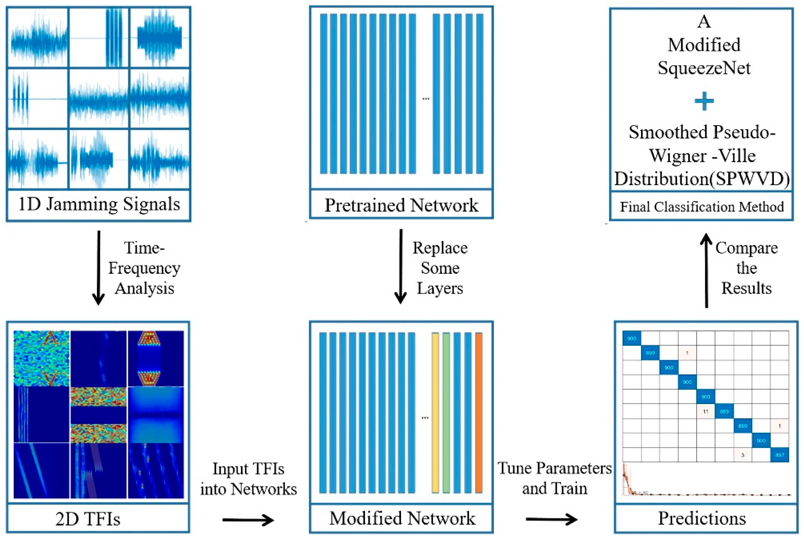
Figure 1. Flowchart of the transfer learning-based classification method.
Symmetry 14 02318 g001
Figure 2. Modification of the SqueezeNet’s last six layers.
Symmetry 14 02318 g002
Figure 3. The real-part waveforms of 1D active jamming signals. In each subgraph, the abscissa is discrete time, and the ordinate is normalized amplitude. (a) Signal without jamming, (b) Interrupted sampling repeater jamming, (c) Dense false target jamming, (d) Smart noise jamming, (e) Blocking jamming, (f) Spot jamming, (g) Linear sweep jamming, (h) DFTJ + SNJ, (i) ISRJ + LSJ.
Symmetry 14 02318 g003
Figure 4. The steps of TFI processing.
Symmetry 14 02318 g004
Figure 5. Three kinds of TFIs for nine types of radar-jamming signals. (a) Pure noise, (b) ISRJ, (c) DFTJ, (d) SNJ, (e) BJ, (f) SJ, (g) LSJ, (h) DFTJ + SNJ, (i) ISRJ + LSJ.
Symmetry 14 02318 g005
Figure 6. Comparison of two pretrained networks using WVD.
Symmetry 14 02318 g006
Figure 7. Memory usage comparison of the two networks.
Symmetry 14 02318 g007
Figure 8. Comparison of confusion matrices using three kinds of TFIs.
Symmetry 14 02318 g008
Table 1. Simulation settings of jamming signals.
JammingParameterValue
ISRJJNR30~60 dB
Sampling duration5~10 μs
Pulse repetition 1~4
DFTJJNR30~60 dB
False targets3~5
False target delay1~10 μs
SNJJNR30~60 dB
Sampling duration5~10 μs
Pulse repetition 1~4
BJJNR30~60 dB
Jamming bandwidth50~80 MHz
SJJNR30~60 dB
Jamming bandwidth20~40 MHz
LSJJNR30~60 dB
Sweep bandwidth20 MHz
Sweep cycle40~80 μs
JNR: Jamming-to-noise ratio.
Table 2. The modification of SqueezeNet’s last six layers.
LayerChanged (Y/N)Note
End-5DropY60% dropout
End-4ConvYnine 1-by-1 convolutions
End-3ReLUNReLU
End-2PoolN2-D global average pooling
End-1ProbNsoftmax
EndOutputY1 × 9
Table 3. Accuracy comparison of two methods with 1% data for training.
JammingWVDSPWVD
a99.98 ± 0.04100.0 ± 0.00
b83.50 ± 0.0099.86 ± 0.26
c100.0 ± 0.00100.0 ± 0.00
d100.0 ± 0.0096.30 ± 3.14
e100.0 ± 0.00100.0 ± 0.00
f100.0 ± 0.0097.60 ± 0.40
g99.16 ± 1.6599.90 ± 0.14
h99.96 ± 0.0598.38 ± 0.61
i96.88 ± 3.9798.34 ± 2.53
OA (%)97.71 ± 0.3898.92 ± 0.49
Training ratio: 1%, Training: 10 epochs, Learning rate: 0.0005.
Table 4. OA comparison of WVD and SPWVD in different training ratios.
Training Ratio
TFIs0.5%1%3%5%
WVD89.07 ± 1.2197.71 ± 0.3899.82 ± 0.0699.88 ± 0.02
SPWVD91.98 ± 0.7698.92 ± 0.4999.41 ± 0.0499.79 ± 0.12
Training: 10 epochs, Learning rate: 0.0005.
Publisher’s Note: MDPI stays neutral with regard to jurisdictional claims in published maps and institutional affiliations.