Quantum Explosions of Black Holes and Thermal Coordinates

Abstract

The Hawking temperature for a Schwarzschild black hole is $T=1/8\pi M$, where M is the black hole mass. This formula is derived for a fixed Schwarzschild background metric, where the mass M could be arbitrary small. Note that, for vanishing $M\to 0$, the temperature T becomes infinite. However, the Schwarzschild metric itself is regular when the black hole mass M tends to zero; it is reduced to the Minkowski metric, and there are no reasons to believe that the temperature becomes infinite. We point out that this discrepancy may be due to the fact that the Kruskal coordinates are singular in the limit of the vanishing mass of the black hole. To elucidate the situation, new coordinates for the Schwarzschild metric are introduced, called thermal coordinates, which depend on the black hole mass M and the parameter b. The parameter b specifies the motion of the observer along a special trajectory. The thermal coordinates are regular in the limit of vanishing black hole mass M. In this limit, the Schwarzschild metric is reduced to the Minkowski metric, written in coordinates dual to the Rindler coordinates. Using the thermal coordinates, the Schwarzschild black hole radiation is reconsidered, and it is found that the Hawking formula for temperature is valid only for large black holes, while for small black holes, the temperature is $T=1/2\pi (4M+b)$. The thermal observer in Minkowski space sees radiation with temperature $T=1/2\pi b$, similar to the Unruh effect with non-constant acceleration. The thermal coordinates for more general spherically symmetric metrics, including the Reissner–Nordstrom, de Sitter, and anti-de Sitter, are also considered. In these coordinates, one sees a Planck distribution with constant temperature. One obtains that the thermal Planck distribution of massless particles is not restricted to the cases of black holes or constant acceleration, but is valid for any spherically symmetric metric written in thermal coordinates.

1. Introduction

Hawking showed that black holes emit radiation like black bodies with a temperature of $T_H=1/8\pi M$, where M is the mass of the black hole [1,2]. This formula is derived for a fixed Schwarzschild background metric, where the mass M could be arbitrary small. Note that, for vanishing $M\to 0$, the temperature T becomes infinite. However, the Schwarzschild metric itself is regular when the black hole mass M tends to zero; it is reduced to the Minkowski metric, and there are no reasons to believe that the temperature becomes infinite. We point out that this discrepancy may be due to the fact that the Kruskal coordinates are singular in the limit of the vanishing mass of the black hole.

We emphasize that, in the present paper, we do not discuss the dynamical evaporation process of the black hole with its well-known problems of back reaction and quantum gravity corrections at the Planck scales. We discuss the question of how it happens that, in the simple model, when we have the classical Schwarzschild background and free quantum fields, it turns out that the temperature is singular in the limit of a vanishing black hole mass. From Hawking’s formula, it follows that the energy density of radiation emitted by a black hole according to the Stefan–Boltzmann formula behaves at small M as $M^{-4}$. Therefore, if $M\to 0$, the black hole releases an infinite amount of energy, which is clearly not physical. This can be called the problem of the big bang of black holes. The information loss problem [3,4,5] may be closely related to this big bang problem, since the radiation entropy diverges for small M as $M^{-3}$. Considerations in more complicated cases, such as a de Sitter–Schwarzschild black hole, do not improve the situation in an essential way.

Standard transformation from the Schwarzschild coordinates to the Kruskal ones includes first transformation from the Schwarzschild coordinates to Eddington–Finkelstein coordinates [6,7,8,9]. The Schwarzschild metric in the Schwarzschild coordinates:

$$d{s}^2=-(1-\frac{2M}{r})d{t}^2+{(1-\frac{2M}{r})}^{-1}d{r}^2+r^{2}d{\mathsf{\Omega }}^2,r>2M>0,$$

(1)

obviously admits the $M\to 0$ limit, which defines Minkowski space. The Kruskal coordinates $(U,V)$ are defined as

$$\begin{array}{ccc}\hfill U& =& -e^{-u/4M},V=e^{v/4M}\hfill \end{array}$$

(2)

Here, u and v are the Eddington–Finkelstein coordinates. The Kruskal coordinates are used to obtain the maximal analytic extension, but we note that, in the limit of a vanishing black hole mass M, even outside of the horizon, $r>2M$, the Kruskal coordinates and the metric result in a singularity, instead of becoming the Minkowski one. This leads also to the singular behavior of the Hawking temperature $T_H=1/8\pi M$ in the limit $M\to 0$. To improve the situation, exponential (E)-coordinates $𝒰$ and $𝒱$ for the Schwarzschild metric are introduced:

$$\begin{array}{c}\hfill 𝒰=-e^{-\frac{u}{4M+b}},𝒱=e^{\frac{v}{4M+b}},\end{array}$$

(3)

which depend on the black hole mass M and a parameter $b>0$. This parameter b sets the observer’s motion along a special trajectory. The E-coordinates are regular in the limit of the vanishing black hole mass M. Obviously, in this limit, the Schwarzschild metric is reduced to the Minkowski one written in the E-coordinates.

Black hole radiation was considered, and it was found that the Hawking formula for temperature is approximately valid only for large black holes, while for small black holes, for the temperature of the black hole, the following formula is obtained:

$$T=\frac{1}{2\pi (4M+b)}.$$

(4)

As a result, black holes could completely evaporate in terms of classical geometry, but it is shown that this requires infinite time because the mass is decreasing in inverse proportion to time,

$$M\left(t\right)=\frac{C}{t},t\to \infty$$

(5)

We show that the E-observer in Minkowski space will see radiation with the temperature:

$$T=\frac{1}{2\pi b}.$$

(6)

This effect is similar (dual) to the Unruh effect [10,11] for the Rindler metric [12], but in our case, the acceleration is not a constant.

We define the E-coordinates $(𝒰,𝒱)$ and logarithmic (L)-coordinates $(\nu ,\vartheta )$ for the arbitrary static metric of the form:

$$d{s}^2=-f\left(r\right)d{t}^2+f{\left(r\right)}^{-1}d{r}^2+r^{2}d{\mathsf{\Omega }}^2=-f\left(r\right)dudv+r^{2}d{\mathsf{\Omega }}^2$$

(7)

as

$$𝒰=-e^{-\frac{u}{B}},𝒱=e^{\frac{v}{B}},B>0,$$

(8)

$$\vartheta =\frac{1}{a}log\left(av\right),\nu =-\frac{1}{a}log(-au)a>0.$$

(9)

It is shown that one has the Planck distribution with temperature $T=1/2\pi B$ and $T=a/2\pi$ for quantum fields in the gravitational background (7) with an arbitrary function $f\left(r\right)$ in E- and L-coordinates, respectively. We have the following general scheme (duality):

$$\begin{array}{c}\hfill \left(\begin{array}{c}E-coord.\\ (𝒰,𝒱)\end{array}\right)\underset{𝒰=-e^{-\frac{u}{B}}}{\overset{𝒱=e^{\frac{v}{B}}}{\leftarrow }}\left(\begin{array}{c}\mathcal{M}\\ (u,v)\\ d{s}_2^2=-f\left(r\right)dudv\end{array}\right)\underset{\vartheta =\frac{1}{a}log\left(av\right)}{\overset{\nu =-\frac{1}{a}log(-au)}{\to }}\left(\begin{array}{c}\mathrm{L}\text{-}\mathrm{coord}.\\ (\nu ,\vartheta )\end{array}\right)\end{array}$$

(10)

The physical meaning of the above formulae for temperature is that they give the temperature of radiation for different observers moving along different trajectories in the same background. The simplest examples of such special trajectories are the ones in Minkowski space. The standard Rindler observer moves with constant acceleration and sees radiation from the Minkowski vacuum as it has a temperature defined by its acceleration. The E-observer moves along a hyperbola and feels the temperature. The E- and L-coordinates can be called the thermal coordinates, since in these coordinates, one sees a Planck distribution with constant temperature. In fact, the property of having a temperature is associated not only with black holes, but using the thermal coordinates, that is the temperature can be obtained for any metric. The implications for the information loss problem and primordial black holes are mentioned.

The paper is organized as follows. We start with Section 2, reminding about the standard definition of the Kruskal coordinates, and also, we discuss the problem that arises with them when one considers the limit $M\to 0$. Then, in Section 2.2, we introduce in the E-coordinates for the Schwarzschild metric and, in Section 2.3 the temperature of Schwarzschild black holes in the E-coordinates. In the next Section 3, we discuss the E-coordinates in Minkowski space. We show in Section 3.1 that two-dimensional Minkowski space can be represented as a union of four disconnected regions, right (R), future (F), left (L), and past (P), and each of them is isometric to two-dimensional Minkowski space. In Section 3.2, we study geodesics in the E-coordinates. In Section 3.3, we calculate the acceleration of an E-observer. Section 3.4 is devoted to the comparison of the E- and Rindler coordinates in Minkowski space. In Section 4, we introduce the general E-coordinates. In Section 4.2, accelerations along special trajectories $\mathcal{X}={\mathcal{X}}_0$ in black hole backgrounds are calculated. Then, in the next sections, we consider some examples. In Section 5, the general L-coordinates are introduced. In Section 5.4 the temperature in the L-coordinates is calculated, and it is found that it is given by a universal formula that does not depend on the characteristics of the black hole under consideration. The origin of this phenomena is that the choice of the coordinate system depends essentially on the metric itself. In Section 6, we present an estimation of the evaporation time as can been seen by observers in different coordinate systems. In Section 7, we summarize the obtained results and discuss their physical applications.

2. Exponential Coordinates

2.1. Kruskal Coordinates

Standard transformation from the Schwarzschild coordinates to the Kruskal ones includes first transformation from the Schwarzschild coordinates to the Eddington–Finkelstein coordinates. The Schwarzschild metric in the Schwarzschild coordinates is

$$d{s}^2=-(1-\frac{2M}{r})d{t}^2+{(1-\frac{2M}{r})}^{-1}d{r}^2+r^{2}d{\mathsf{\Omega }}^2,r>2M>0.$$

(11)

where $d{\mathsf{\Omega }}^2=d{\theta }^2+{sin}^2\theta d{\phi }^2$. It is obvious that the exterior Schwarzschild spacetime ($r>r_h=2M$) admits the $M\to 0$ limit, which defines Minkowski spacetime. Note that the Kretschmann invariant $K=\frac{48M^2}{r^6}\to 0$ as $M\to 0$ for any fixed $r>2M$.

One can introduce the tortoise coordinate $r_{*}$:

$$r_{*}=r+2Mlog\left(\frac{r}{2M}-1\right),$$

(12)

which solves the equation $d{r}_{*}={(1-2M/r)}^{-1}dr$. To keep the reality condition, one has to assume $r>2M$. Then, one defines

$$\begin{array}{c}\hfill u=t-r_{*},v=t+r_{*}.\end{array}$$

(13)

(coordinates $u,v$ cover the whole ${\mathbb{R}}^2$), and one has

$$d{s}_2^2=-(1-\frac{2M}{r})d{t}^2+{(1-\frac{2M}{r})}^{-1}d{r}^2=-(1-\frac{2M}{r})dudv$$

(14)

The Kruskal coordinates are

$$\begin{array}{ccc}\hfill U& =& -e^{-\frac{u}{4M}},V=e^{v/4M}\hfill \end{array}$$

(15)

and the Schwarzschild metric becomes

$$\begin{array}{c}\hfill d{s}^2=-\frac{32M^3}{r}{e}^{-r/2M}dUdV+r^{2}d{\mathsf{\Omega }}^2,\end{array}$$

(16)

where r is defined by equation

$$\begin{array}{c}\hfill \left(\frac{r}{2M}-1\right)e^{\frac{r}{2M}}=-UV\end{array}$$

(17)

Note that the Kruskal coordinates (15) and metric (16) are singular in the limit $M\to 0$.

2.2. E-Coordinates for the Schwarzschild Metric

To be able to send the mass M of a black hole to zero, we define coordinates (we call them the E-coordinates) as follows

$$\begin{array}{ccc}\hfill 𝒰& =& -e^{-\frac{u}{4M+b}},𝒱=e^{\frac{v}{4M+b}};\hfill \end{array}$$

(18)

here, b is a positive constant. The coordinates run over the region $𝒰<0,𝒱>0$. The question of the existence of an extension of the Schwarzschild metric that is analytic, not only with respect to the space and time variables, but also with respect to the mass parameter requires a separate consideration.

The Schwarzschild metric in the E-coordinates is ($r>2M$)

$$\begin{array}{ccc}\hfill d{s}^2& =& -(1-\frac{2M}{r})d{t}^2+{(1-\frac{2M}{r})}^{-1}d{r}^2+r^{2}d{\mathsf{\Omega }}^2\hfill \\ & =& {(4M+b)}^2(1-\frac{2M}{r})\frac{d𝒰d𝒱}{𝒰𝒱}+r^{2}d{\mathsf{\Omega }}^2;\hfill \end{array}$$

(19)

here, r is derived from the relation:

$$e^{2r_{*}/(4M+b)}=-𝒰𝒱.$$

(20)

It is clear that, in the limit $b\to 0$ the metric (19), rewritten as

$$\begin{array}{ccc}\hfill d{s}^2& =& -16{(M+b/4)}^2{\left(2M\right)}^{\frac{M}{M+b/4}}\frac{{(r-2M)}^{\frac{b}{4M+b}}}{r}{e}^{-\frac{r}{2(M+b/4)}}·d𝒰d𝒱+r^{2}d{\mathsf{\Omega }}^2\hfill \end{array}$$

(21)

becomes the Schwarzschild–Kruskal metric (16).

At the limit $M\to 0$, the metric (19) becomes

$$\begin{array}{ccc}\hfill d{s}^2& =& -b^2{e}^{-\frac{2r}{b}}d𝒰d𝒱+r^{2}d{\mathsf{\Omega }}^2;\hfill \end{array}$$

(22)

here, r is defined by

$$-𝒰𝒱=e^{\frac{2r}{b}}.$$

(23)

Equation (23) is nothing but the formula (20) rewritten as

$${(r-2M)}^{\frac{M}{M+b/4}}={\left(2M\right)}^{M/(M+b/4)}(-𝒰𝒱)e^{-\frac{r}{2(M+b/4)}}$$

(24)

in the limit $M\to 0$. An explicit check shows that the metric (22) is the Minkowski metric.

2.3. Temperature of Schwarzschild Black Holes in E-Coordinates

We consider the scaler field on the Schwarzschild background in two systems of coordinates, the Eddington–Finkelstein $(u,v)$ and E-coordinates $(𝒰,𝒱)$, related as

$$𝒰=-exp\{-\frac{u}{4M+b}\},𝒱=exp\left\{\frac{v}{4M+b}\right\},u,v\in \mathbb{R},M>0,b>0.$$

(25)

The two-dimensional parts of the Schwarzschild metric in these coordinate systems read

$$\begin{array}{ccc}\hfill d{s}_2^2& =& -(1-\frac{2M}{r})dudv={(4M+b)}^2(1-\frac{2M}{r})\frac{d𝒰d𝒱}{𝒰𝒱},r>2M.\hfill \end{array}$$

(26)

The wave equations for the scalar field $\varphi (u,v)=\mathsf{\Phi }(𝒰,𝒱)$ in these coordinate systems are

$$\begin{array}{ccc}\hfill {\partial }_v{\partial }_u\varphi & =& 0,u,v\in \mathbb{R}\hfill \end{array}$$

(27)

$$\begin{array}{ccc}\hfill {\partial }_{𝒱}{\partial }_{𝒰}\mathsf{\Phi }& =& 0,𝒰<0,𝒱>0.\hfill \end{array}$$

(28)

They can be represented as combinations of the left and write modes, $\varphi (u,v)={\varphi }_R\left(u\right)+{\varphi }_L\left(v\right)$. For the real right mode (for the left mode, all considerations are similar and will be omitted), one has

$$\begin{array}{ccc}\hfill {\varphi }_R\left(u\right)& =& {\int }_0^{\infty }d\omega (f_{\omega }{b}_{\omega }+f_{\omega }^{*}{b}_{\omega }^{+}),f_{\omega }\left(u\right)=\frac{1}{\sqrt{4\pi \omega }}{e}^{-i\omega u},\hfill \end{array}$$

(29)

where

$$[b_{\omega },b_{{\omega }^{\prime }}^{+}]=\delta (\omega -{\omega }^{\prime }).$$

(30)

One also has representation for the $\mathsf{\Phi }$-field $\mathsf{\Phi }(𝒰,\mathcal{V})={\mathsf{\Phi }}_R\left(𝒰\right)+{\mathsf{\Phi }}_L\left(\mathcal{V}\right)$ where, for the right mode (similar for the left one),

$$\begin{array}{ccc}\hfill {\mathsf{\Phi }}_R\left(𝒰\right)& =& {\int }_0^{\infty }d\mu \left({\mathfrak{b}}_{\mu }{\mathfrak{f}}_{\mu }\left(𝒰\right)+{\mathfrak{b}}_{\mu }^{+}{\mathfrak{f}}_{\mu }^{*}\left(𝒰\right)\right),{\mathfrak{f}}_{\mu }\left(𝒰\right)=\frac{1}{\sqrt{4\pi \mu }}{e}^{-i\mu 𝒰}\hfill \end{array}$$

(31)

where

$$[{\mathfrak{b}}_{\mu },{\mathfrak{b}}_{{\mu }^{\prime }}]=\delta (\mu -{\mu }^{\prime })$$

(32)

Right (and left) modes in different coordinate systems are related ${\varphi }_R\left(u\right)={\mathsf{\Phi }}_R\left(𝒰\left(u\right)\right)$, and therefore,

$$\begin{array}{ccc}\hfill {\int }_0^{\infty }d\omega (f_{\omega }{b}_{\omega }+f_{\omega }^{*}{b}_{\omega }^{+})& =& {\int }_0^{\infty }d\mu ({\mathfrak{f}}_{\mu }{\mathfrak{b}}_{\mu }+{\mathfrak{f}}_{\mu }^{*}{\mathfrak{b}}_{\mu }^{+}),u\in \mathbb{R}\hfill \end{array}$$

(33)

Multiplying (33) by $f_{{\omega }^{\prime }}\left(u\right)$ and integrating the first equation over $\mathbb{R}$, one obtains (for $b=0$, we obtain the standard formula for the Schwarzschild metric in the Kruskal coordinates)

$$\begin{array}{ccc}\hfill b_{\omega }=\int d\mu \left({\beta }_{\omega \mu }^{*}{\mathfrak{b}}_{\mu }^{+}+{\alpha }_{\omega \mu }^{*}{\mathfrak{b}}_{\mu }\right),b_{\omega }^{+}& =& \int d\mu \left({\beta }_{\omega \mu }{\mathfrak{b}}_{\mu }+{\alpha }_{\omega \mu }{\mathfrak{b}}_{\mu }^{+}\right),\hfill \end{array}$$

(34)

where

$$\begin{array}{ccc}\hfill {\beta }_{\omega \mu }& =& {\int }_{\mathbb{R}}\frac{du}{2\pi }\sqrt{\frac{\omega }{\mu }}{e}^{-i\omega u}{e}^{-i\mu 𝒰},\hfill \end{array}$$

(35)

$$\begin{array}{ccc}\hfill {\alpha }_{\omega \mu }& =& {\int }_{\mathbb{R}}\frac{du}{2\pi }\sqrt{\frac{\omega }{\mu }}{e}^{-i\omega u}{e}^{i\mu 𝒰}.\hfill \end{array}$$

(36)

The E-observer has the E-vacuum

$${\mathfrak{b}}_{\omega }|0_E⟩=0,$$

(37)

i.e., the state $|0_E⟩$ does not contain $\mathfrak{b}$ particles. However, it contains the Minkowski b particles:

$$⟨0_E|N_{\omega }\left(b\right)|0_E⟩\equiv ⟨0_E|b_{\omega }^{+}{b}_{\omega }|0_E⟩={\int }_0^{\infty }d\mu {|{\beta }_{\omega \mu }|}^2.$$

(38)

The Bogoliubov coefficient ${\beta }_{\omega \nu }$ is given by (35) with $𝒰$ as in (25), and we have

$$\begin{array}{c}\hfill {\beta }_{\omega \mu }=\frac{B}{2\pi }\sqrt{\frac{\omega }{\mu }}{e}^{-\frac{\pi B\omega }{2}}{\left(\mu \right)}^{-iB\omega }\mathsf{\Gamma }\left(iB\omega \right),B=4M+b\end{array}$$

(39)

Using the formula ${\left|\mathsf{\Gamma }\left(ix\right)\right|}^2=\pi /(xsinh\left(\pi x\right))$, we obtain the Planck distribution

$$\begin{array}{ccc}\hfill |{\beta }_{\omega \mu }{|}^2& =& \frac{B}{2\pi \mu }\frac{1}{e^{2\pi B\omega }-1},\hfill \end{array}$$

(40)

with the temperature

$$T=\frac{1}{2\pi B}=\frac{1}{2\pi (4M+b)}$$

(41)

3. E-Coordinates in Minkowski Space

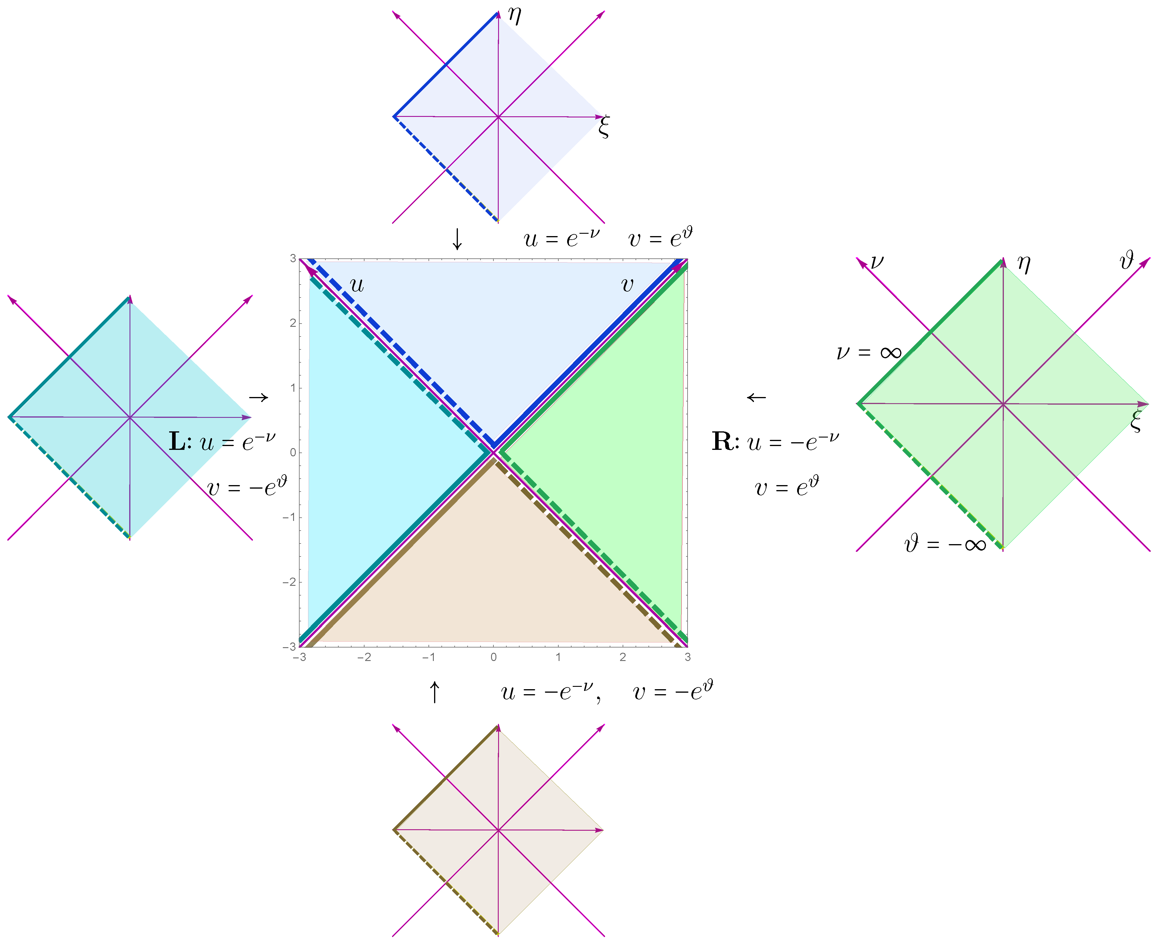
3.1. Minkowski Space in Terms of New Coordinates $\mathcal{U},\mathcal{V}$ and $\mathcal{T},\mathcal{X}$

Starting from the Minkowski coordinates:

$$d{s}^2=d{s}_2^2+r^{2}d{\mathsf{\Omega }}^2,d{s}_2^2=-d{t}^2+d{r}^2,r\in {\mathbb{R}}_{+},t\in \mathbb{R}.$$

(42)

we introduce the E-ones:

$$\begin{array}{ccc}\hfill \mathcal{U}& =& {\mathcal{U}}^{\left(R\right)}(t,r)=-exp\left\{\frac{r-t}{b}\right\}=-exp\{-\frac{u}{b}\},u=t-r\hfill \end{array}$$

(43)

$$\begin{array}{ccc}\hfill \mathcal{V}& =& {\mathcal{V}}^{\left(R\right)}(t,r)=exp\left\{\frac{t+r}{b}\right\}=exp\left\{\frac{v}{b}\right\},v=t+r,b>0,\hfill \end{array}$$

(44)

$r>0$ corresponds to $\mathcal{U}\mathcal{V}<-1$. One has an expression of r in terms of coordinates $\mathcal{U},\mathcal{V}$:

$$r=b/2log(-\mathcal{U}\mathcal{V})$$

(45)

The two-dimensional Minkowski metric in (42) after this change becomes

$$\begin{array}{c}\hfill d{s}_2^2=b^2\frac{d\mathcal{U}d\mathcal{V}}{\mathcal{U}\mathcal{V}}\end{array}$$

(46)

One can see that the metric (22) admits an extension to the region $-\mathcal{U}\mathcal{V}<0$. In this case, by using Formula (45), the coordinate r is extended to the region $r\le 0$; see Figure 1.

Figure 1. Map of 4 copies ${\mathbb{M}}^{1,1}$. Here, $b=1$.

We also define the coordinates:

$$\mathcal{T}=\frac{\mathcal{U}+\mathcal{V}}{2},\mathcal{X}=\frac{\mathcal{V}-\mathcal{U}}{2}$$

(47)

We cover the R-region:

$$\begin{array}{ccc}\hfill \mathbf{R}& =& \{(\mathcal{T},\mathcal{X})\in {\mathbb{R}}^2|{\mathcal{X}}^2-{\mathcal{T}}^2>0,\mathcal{X}>0\}\hfill \end{array}$$

by the map

$$\begin{array}{ccc}\hfill R& :& \mathcal{T}=e^{r/b}sinh\frac{t}{b},\mathcal{X}=e^{r/b}cosh\frac{t}{b},(t,x)\in {\mathbb{M}}^{(1,1)}\hfill \end{array}$$

(48)

The inverse transformation is

$$\begin{array}{ccc}\hfill t& =& barctanh\frac{\mathcal{T}}{\mathcal{X}}r=b/2log({\mathcal{X}}^2-{\mathcal{T}}^2),(\mathcal{T},\mathcal{X})\in \mathbf{R}\hfill \end{array}$$

(49)

The metric here is

$$d{s}_2^2=-d{t}^2+d{r}^2=\frac{b^2}{{\mathcal{X}}^2-{\mathcal{T}}^2}(-d{\mathcal{T}}^2+d{\mathcal{X}}^2).$$

(50)

Let us introduce the future (F) E-coordinates:

$$\begin{array}{c}\hfill \mathcal{U}={\mathcal{U}}^{\left(F\right)}(r,t)=exp\left\{\frac{r-t}{b}\right\}=exp\{-\frac{u}{b}\},\mathcal{V}={\mathcal{V}}^{\left(F\right)}(r,t)=exp\left\{\frac{t+r}{b}\right\}=exp\left\{\frac{v}{b}\right\},\end{array}$$

(51)

and they cover the F-part of the $(\mathcal{U},\mathcal{V})$-plane (see the top part of Figure 1):

$$\mathcal{U}\mathcal{V}>0.$$

(52)

The Minkowski metric (42) after (51) becomes

$$\begin{array}{c}\hfill d{s}_2^2=-b^2\frac{d\mathcal{U}d\mathcal{V}}{\mathcal{U}\mathcal{V}}.\end{array}$$

(53)

One also introduces the left (L) E-coordinates:

$$\begin{array}{c}\hfill \mathcal{U}={\mathcal{U}}^{\left(L\right)}(t,r)=exp\left\{\frac{r-t}{b}\right\}=exp\{-\frac{u}{b}\},\mathcal{V}={\mathcal{V}}^{\left(L\right)}(t,r)=-exp\left\{\frac{t+r}{b}\right\}=-exp\left\{\frac{v}{b}\right\},\end{array}$$

(54)

with the inequality:

$$\mathcal{U}\mathcal{V}<0$$

(55)

and the past (P) E-coordinates:

$$\begin{array}{c}\hfill \mathcal{U}={\mathcal{U}}^{\left(P\right)}(t,r)=-exp\left\{\frac{r-t}{b}\right\}=exp\{-\frac{u}{b}\},\mathcal{V}={\mathcal{V}}^{\left(P\right)}(t,r)=-exp\left\{\frac{t+r}{b}\right\}=-exp\left\{\frac{v}{b}\right\},\end{array}$$

(56)

with the inequality:

$$\mathcal{U}\mathcal{V}>0.$$

(57)

The metric can be written in the universal way:

$$\begin{array}{c}\hfill d{s}_2^2=-dudv=-b^2\frac{d\mathcal{U}d\mathcal{V}}{\left|\mathcal{U}\mathcal{V}\right|},\mathcal{U}\mathcal{V}\ne 0.\end{array}$$

(58)

These maps are shown in Figure 1.

To summarize, we obtained the two-dimensional plane divided into four disconnected regions with E-coordinates $(\mathcal{U},\mathcal{V})$ and the metric given by (58). In other words, we obtained that the two-dimensional space is represented as a union of four disconnected regions R, F, P, and L, each of which is isometric to two-dimensional Minkowski space.

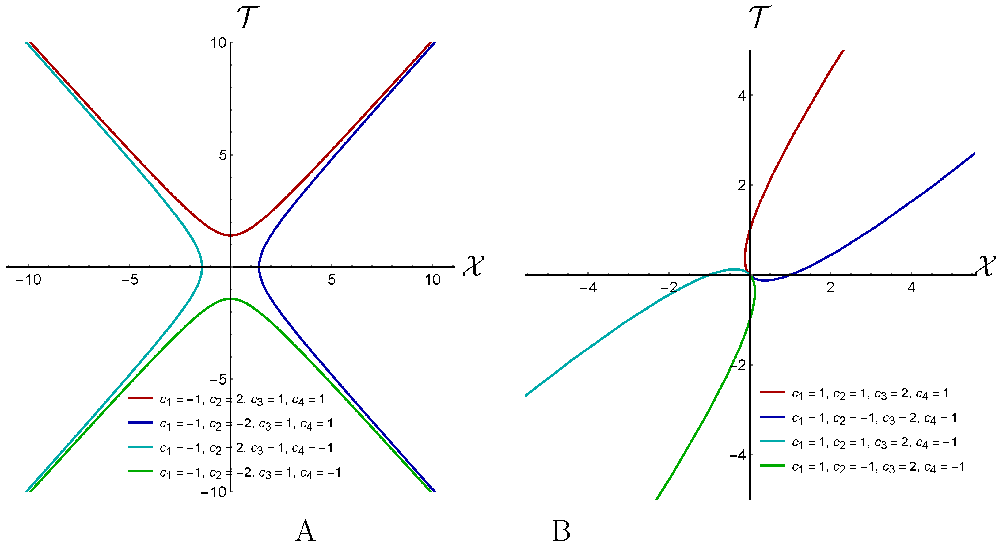
3.2. Geodesics in E-Coordinates

The geodesics in E-coordinates $(\mathcal{U},\mathcal{V})$ can be obtained simply by changing the variables from the geodesics in Minkowski space. However, it seems instructive and useful for quantization to investigate geodesics directly in the E-coordinates. The geodesic equations for the metric (22) are

$$\begin{array}{ccc}\hfill \frac{{\mathcal{V}}^{\prime }{\left(\mathfrak{s}\right)}^2-\mathcal{V}\left(\mathfrak{s}\right){\mathcal{V}}^{″}\left(\mathfrak{s}\right)}{\mathcal{U}\left(\mathfrak{s}\right)\mathcal{V}{\left(\mathfrak{s}\right)}^2}& =& 0,\hfill \end{array}$$

(59)

$$\begin{array}{ccc}\hfill \frac{{\mathcal{U}}^{\prime }{\left(\mathfrak{s}\right)}^2-\mathcal{U}\left(\mathfrak{s}\right){\mathcal{U}}^{″}\left(\mathfrak{s}\right)}{\mathcal{U}{\left(\mathfrak{s}\right)}^2\mathcal{V}\left(\mathfrak{s}\right)}& =& 0.\hfill \end{array}$$

(60)

These geodesic Equations (59) and (60) can be solved to obtain

$$\mathcal{V}\left(\mathfrak{s}\right)=c_2{e}^{c_1\mathfrak{s}},\mathcal{U}\left(\mathfrak{s}\right)=c_4{e}^{c_3\mathfrak{s}};$$

(61)

here, $-\infty <\mathfrak{s}<\infty$.

To guaranty that the geodesics run in one of the regions R, F, L, P, we have to take

$$\begin{array}{c}\hfill \mathbf{R}:c_2>0,c_4<0,\mathbf{F}:c_2>0,c_4>0\end{array}$$

(62)

$$\begin{array}{c}\hfill \mathbf{L}:c_2<0,c_4>0,\mathbf{P}:c_2<0,c_4<0\end{array}$$

(63)

Here, $-\infty <s<\infty$, and $c_1$ and $c_3$ can have any signs.

The geodesics (61) in the $(\mathcal{T},\mathcal{X})$ coordinates are

$$\begin{array}{c}\hfill \mathcal{X}\left(\mathfrak{s}\right)=\frac{1}{2}\left(c_4{e}^{c_3\mathfrak{s}}-c_2{e}^{c_1\mathfrak{s}}\right),\mathcal{T}\left(\mathfrak{s}\right)=\frac{1}{2}\left(c_2{e}^{c_1\mathfrak{s}}+c_4{e}^{c_3\mathfrak{s}}\right).\end{array}$$

(64)

One can check that these geodesics after mapping to $t,x$ (Minkowski space coordinates) are (as should be) the straight lines:

$$\begin{array}{ccc}\hfill t=t\left(\mathfrak{s}\right)& =& b\mathrm{arctanh}\frac{\mathcal{T}\left(\mathfrak{s}\right)}{\mathcal{X}\left(\mathfrak{s}\right)}=\frac{1}{2}\left(\mathfrak{s}(-c_1-c_3))-log\left(-\frac{c_2}{c_4}\right)\right)\hfill \end{array}$$

(65)

$$\begin{array}{ccc}\hfill r=r\left(\mathfrak{s}\right)& =& 2blog(\mathcal{X}{\left(\mathfrak{s}\right)}^2-\mathcal{T}{\left(\mathfrak{s}\right)}^2)=2b\left((c_1+c_3)\mathfrak{s}+log(-c_2{c}_4)\right).\hfill \end{array}$$

(66)

We have three types of geodesics:

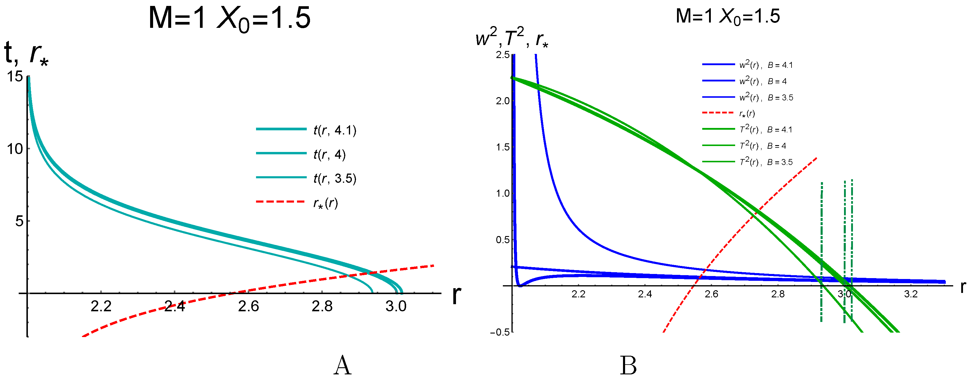
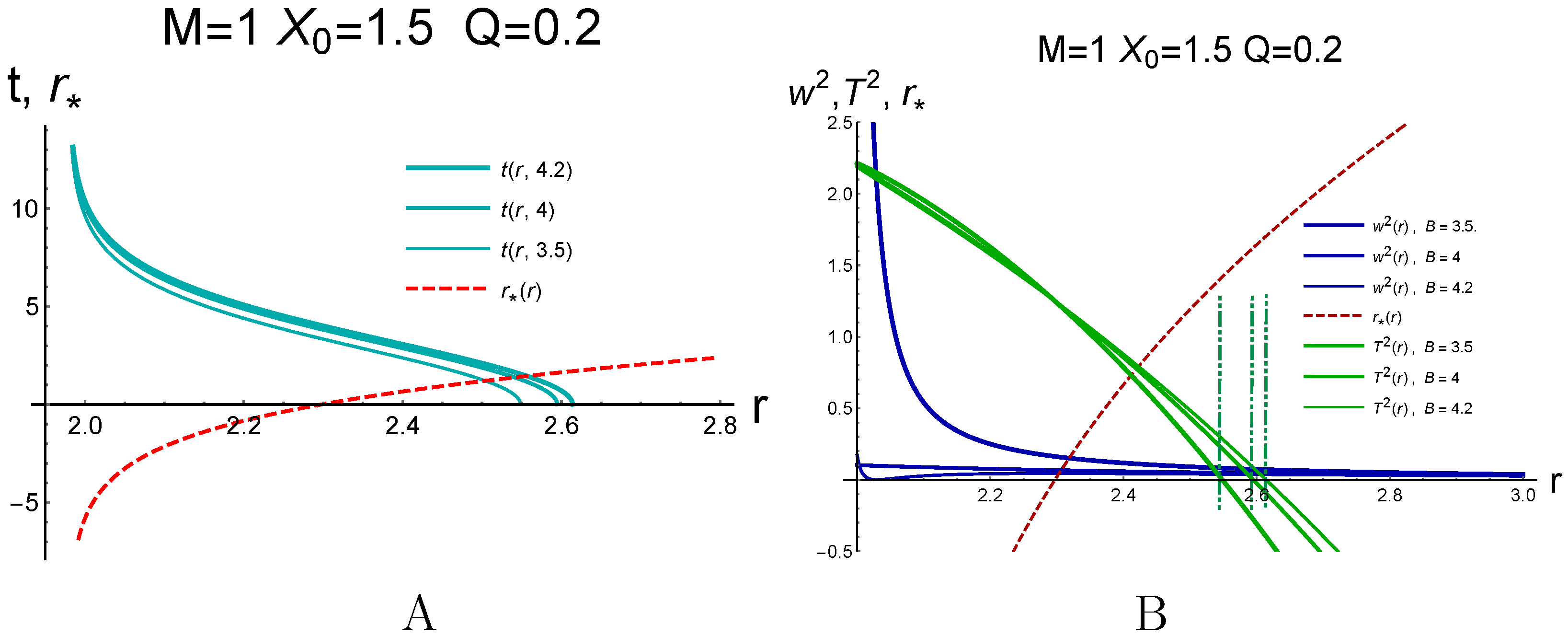
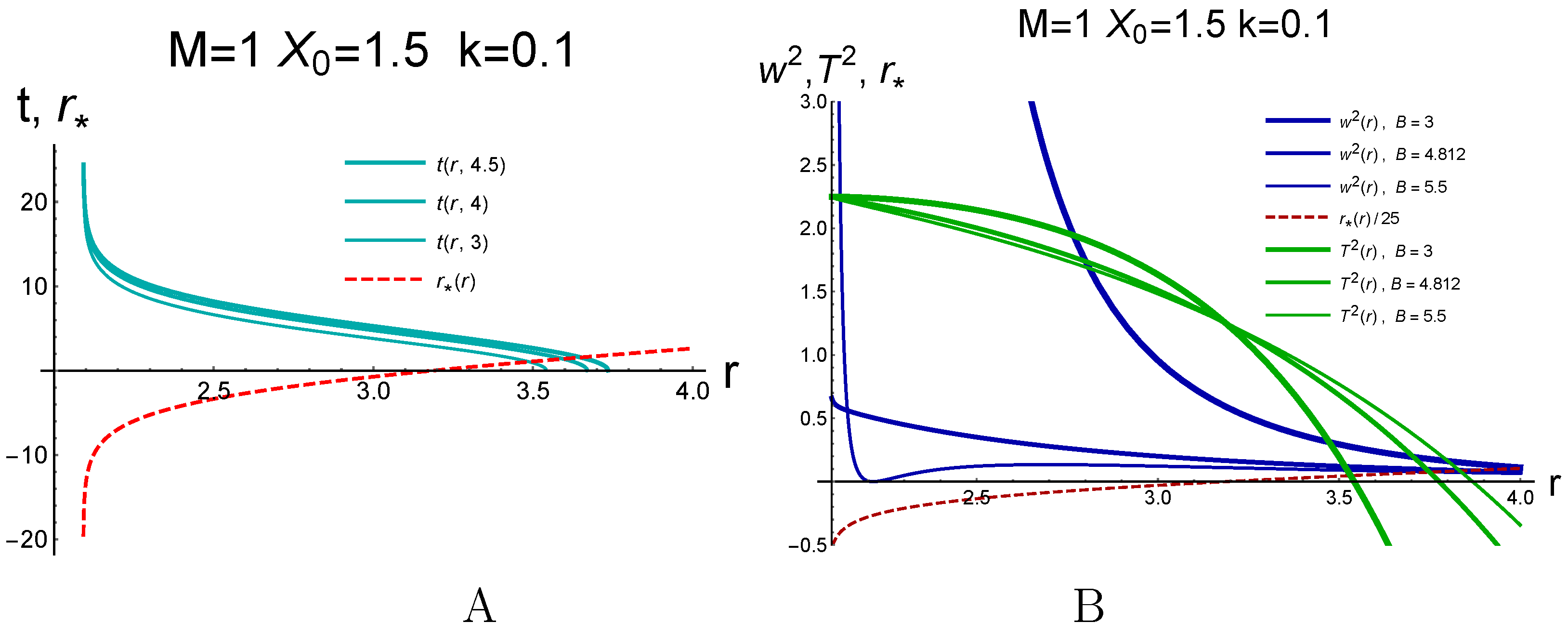
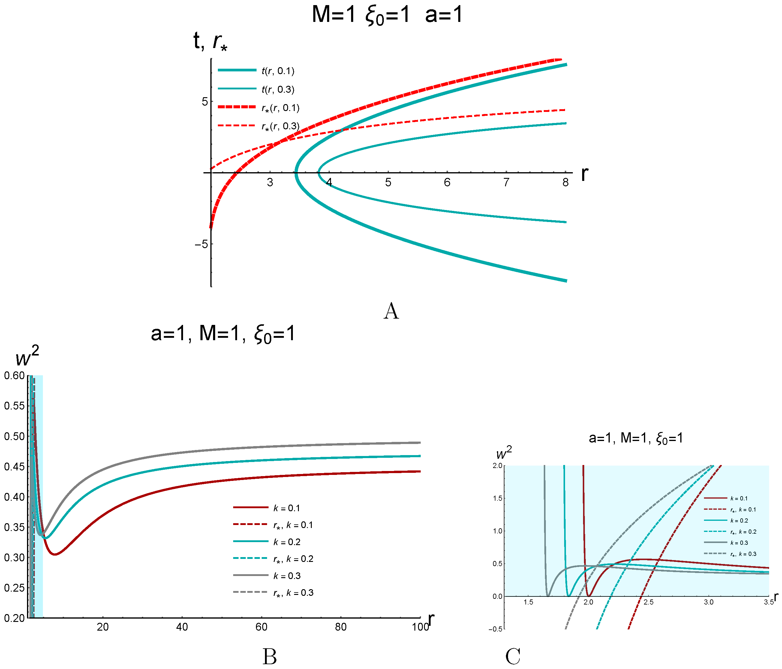
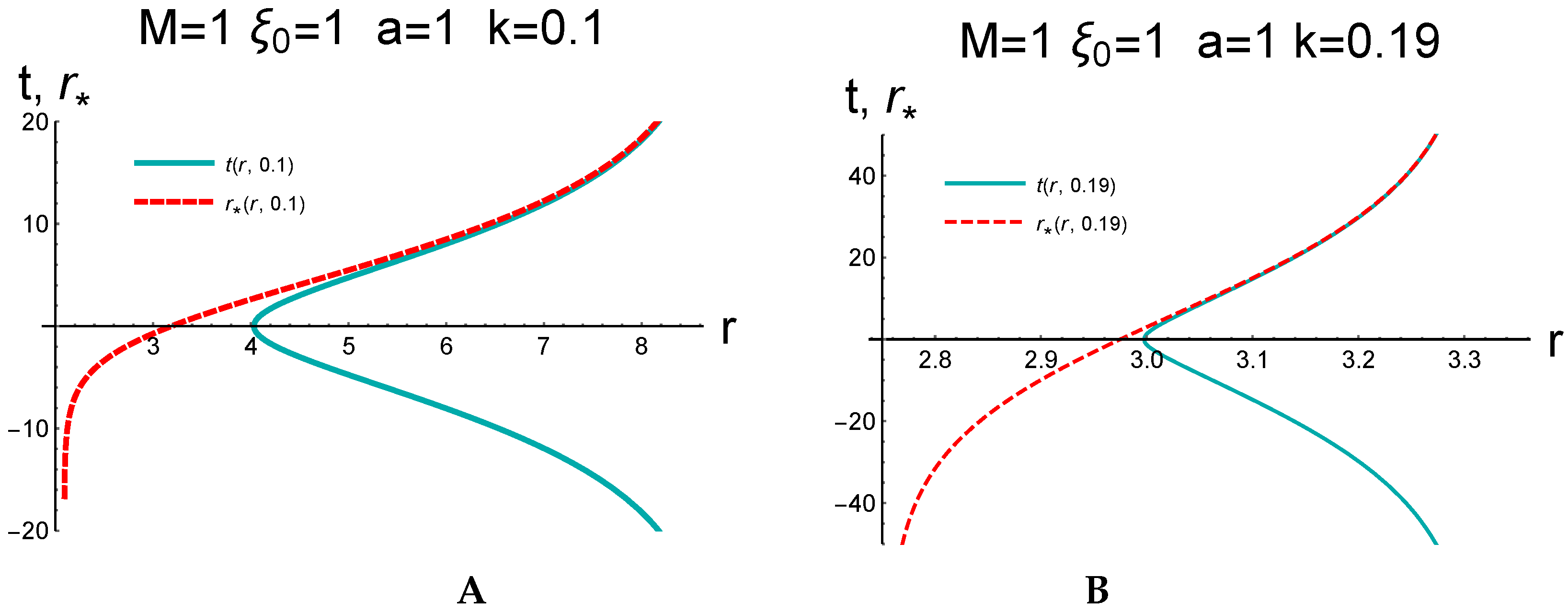
• $c_1{c}_3<0$. In this case, both “ends” of the geodesics are in infinities; see, for example, the plot in Figure 2A.
  

  Figure 2. Geodesics for different values of $c_i,i=1,2,3,4$. (A) For all lines $c_1=-1,c_3=1$ and for dark red line $c_2=2$, $c_4=1$, for blue line $c_2=-2$, $c_4=1$, for green line $c_2=-2$, $c_4=-1$ and for cyan line $c_2=2$, $c_4=-1$. (B) For all lines $c_1=1,c_3=2$ and for dark red line $c_2=1$, $c_4=1$, for blue line $c_2=-1$, $c_4=1$, for green line $c_2=-1$, $c_4=-1$ and for cyan line $c_2=1$, $c_4=-1$.
• $c_1{c}_3>0$. In this case, one “end” of the geodesics is at infinity and the second one is at zero; see, for example, the plot in Figure 2B.
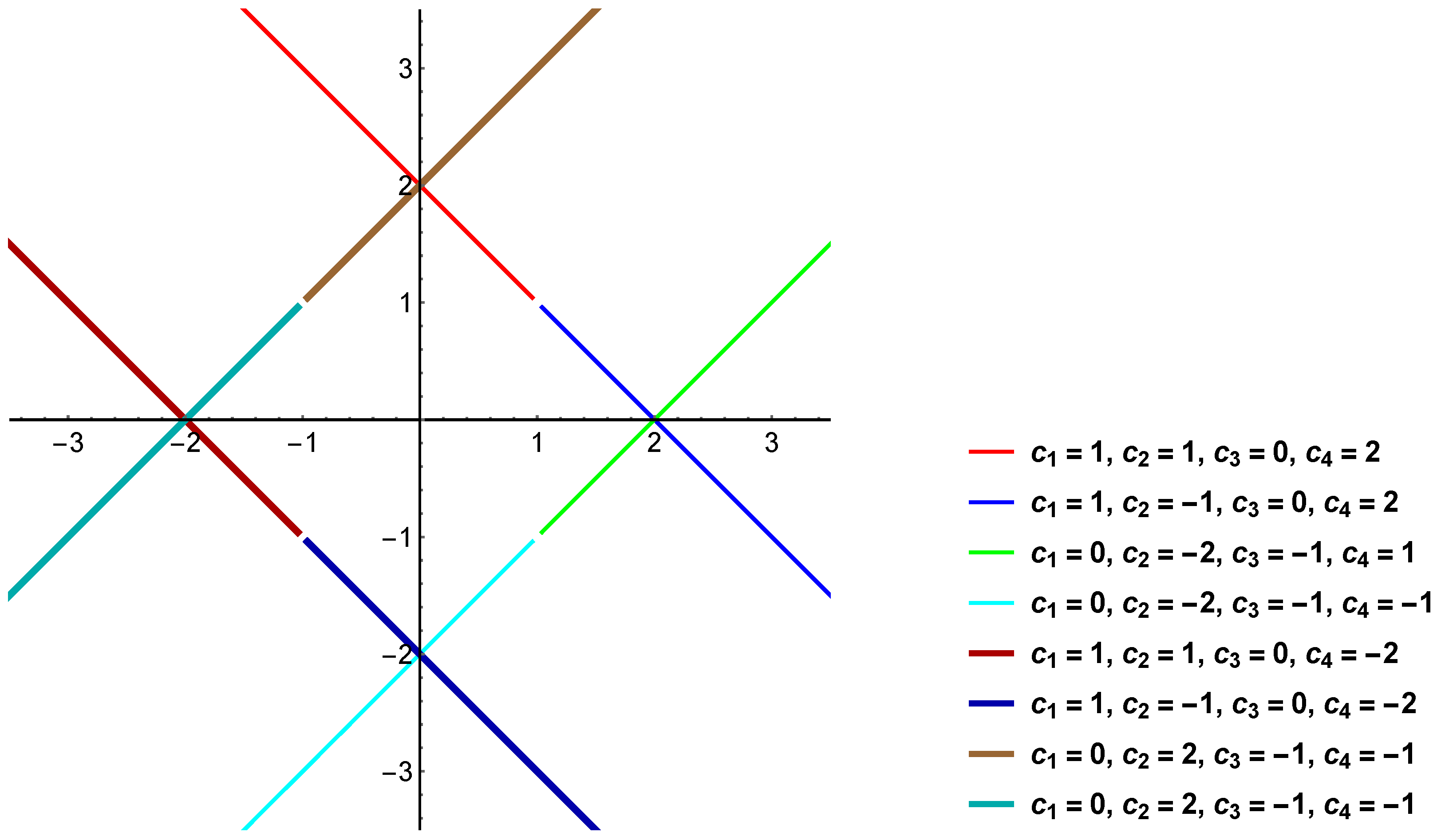
• $c_1=0,c_3\ne 0$ or $c_3=0,c_1\ne 0$. In this case, the geodesics are bounded by the characteristics $\mathcal{U}=0$ or $\mathcal{V}=0$; see Figure 3.
  

  Figure 3. Geodesics for the cases when $c_1$ or $c_3$ is equal to 0.

From (61), it follows that

$${\left(\frac{\mathcal{V}}{c_2}\right)}^{c_3}={\left(\frac{\mathcal{U}}{c_4}\right)}^{c_1}.$$

(67)

3.3. Acceleration in E-Coordinates

Let us consider the time-like trajectory located at $\mathcal{X}={\mathcal{X}}_0$. The proper time $\tau$:

$$\begin{array}{c}\hfill \tau =barctan\left(\frac{\mathcal{T}}{\sqrt{{\mathcal{X}}_0^2-{\mathcal{T}}^2}}\right)+{\tau }_0.\end{array}$$

(68)

From (68), one has

$$\mathcal{T}=\pm {\mathcal{X}}_{0}sin\left(\frac{\tau -{\tau }_0}{b}\right).$$

(69)

We see that it takes the finite time $\mathcal{T}$, or $\tau$, to reach the characteristic $\mathcal{X}=\mathcal{T}$.

In Figure 4A,B, we plot trajectories with ${\mathcal{X}}_0=1$ (red) and ${\mathcal{X}}_0=4$ (blue) in the $(\mathcal{X},\mathcal{T})$ and $(t,x)$ planes, respectively. We can parameterize these trajectories in the Minkowski coordinatesby $\tau$:

$$\begin{array}{ccc}\hfill t& =& b\mathrm{arctanh}\left(sin\left(\frac{\tau -{\tau }_0}{b}\right)\right),\hfill \end{array}$$

(70)

$$\begin{array}{ccc}\hfill r& =& \frac{b}{2}log\left({\mathcal{X}}_0^2{cos}^2\left(\frac{\tau -{\tau }_0}{b}\right)\right).\hfill \end{array}$$

(71)

Figure 4. Trajectories with ${\mathcal{X}}_0=1$ (red) and ${\mathcal{X}}_0=4$ (blue) in the $(\mathcal{X},\mathcal{T})$ plane (A) and $(x,t)$ plane (B). We can take ${\tau }_0=0$.

We obtain

$$\begin{array}{ccc}\hfill V^0& =& \frac{dt}{d\tau }=\frac{{\mathcal{X}}_0}{\sqrt{{\mathcal{X}}_0^2-{\mathcal{T}}^2}},V^1=\frac{dx}{d\tau }=\frac{\mathcal{T}}{\sqrt{{\mathcal{X}}_0^2-{\mathcal{T}}^2}},\hfill \end{array}$$

(72)

$$\begin{array}{ccc}\hfill W^0& =& \frac{d{V}^0}{d\tau }=\frac{{\mathcal{X}}_0\mathcal{T}}{b\left({\mathcal{X}}_0^2-{\mathcal{T}}^2\right)},W^1=\frac{d{V}^1}{d\tau }=\frac{{\mathcal{X}}_0^2}{b\left({\mathcal{X}}_0^2-{\mathcal{T}}^2\right)}.\hfill \end{array}$$

(73)

We have

$$W^2\equiv -{\left(W^0\right)}^2+{\left(W^1\right)}^2=\frac{{\mathcal{X}}_0^2}{b^2\left({\mathcal{X}}_0^2-{\mathcal{T}}^2\right)}.$$

(74)

One can also rewrite (74) in terms of t:

$$\begin{array}{ccc}\hfill W^2& =& \frac{1}{b^2}{cosh}^2\frac{t}{b},\hfill \end{array}$$

(75)

or in term of $\tau$

$$\begin{array}{ccc}\hfill W^2& =& \frac{1}{b^2{cos}^2\left(\frac{\tau -{\tau }_0}{b}\right)}.\hfill \end{array}$$

(76)

These calculations show that the acceleration W of the E-trajectory with “$\mathcal{X}={\mathcal{X}}_0$” in the inertial coordinate system ($t,x$) increases with increasing of the inertial time $t>0$ as $W\sim \frac{1}{b}{e}^{t/b}$. If $b\to 0$, this acceleration increases to infinity, and it decreases to 0 when $b\to \infty$.

The acceleration of the E-observer located at ${\mathcal{X}}_0$ depends on its E-time $\mathcal{T}$ (see Figure 5), as well as it own proper time. The proper time does not depend on the location. In all cases, the acceleration is inversely proportional to the b parameter.

Figure 5. Accelerations of E-observers located at ${\mathcal{X}}_0=1$ (red) and ${\mathcal{X}}_0=2$ (blue) against their E-time $\mathcal{T}$, $b=1$ (A) and proper time $\tau$, $b=0.5$ (gray) and $b=1$ (green) (B).

3.4. Comparison of Exponential and Rindler Coordinates

The accelerated observer traveling in Minkowski spacewith constant acceleration a is described by the Rindler coordinates $(\nu ,\vartheta )$ related to the inertial coordinates $(u,v)$ [11,12]:

$$u=-\frac{1}{a}{e}^{-a\nu },v=\frac{1}{a}{e}^{a\vartheta },a>0.$$

(77)

These transformations define the Rindler observer as an observer that is “at rest” in Rindler coordinates, i.e., maintaining constant $\xi$ and only varying $\eta$; a represents the proper acceleration (along the hyperbola $\xi =0$) of the Rindler observer, whose proper time is defined to be equal to the Rindler coordinate time. The Rindler observer at rest in the $(\eta ,\xi )$ Rindler coordinates travels along the hyperbola:

$$uv=e^{{\xi }_0}$$

(78)

in the inertial coordinates $(t,x)$; see Figure 6.

Figure 6. (A) Rindler observers “at rest” in $\xi$ coordinates (located at $\xi =1,2$) move along hyperbolae in the inertial coordinates with constant acceleration. (B) Rindler observers located at $\xi =1,2$ in $\xi$ coordinates.

The transformation formulas between the inertial coordinates $(t,x)$ and the Rindler coordinates $(\xi ,\eta )$ (for simplicity, we considered the two-dimensional case) are different in the four parts of the inertial coordinates plane ${\mathbb{M}}^{1,1}$. Four different maps of ${\mathbb{M}}^{1,1}$ mapto four different parts of inertial plane [11,12]. Below, we present them in light-cone coordinates $u,v$ and $\nu ,\vartheta$:

$$\begin{array}{ccc}\hfill u& =& t-x,v=t+x,\hfill \end{array}$$

(79)

$$\begin{array}{ccc}\hfill \nu & =& \eta -\xi ,\vartheta =\eta +\xi ,\hfill \end{array}$$

(80)

and

$$\begin{array}{ccc}\hfill \mathbf{R}:u& =& -\frac{1}{a}{e}^{-a\nu },v=\frac{1}{a}{e}^{a\vartheta },\hfill \end{array}$$

(81)

$$\begin{array}{ccc}\hfill \mathbf{F}:u& =& \frac{1}{a}{e}^{-a\nu },v=\frac{1}{a}{e}^{a\vartheta },\hfill \end{array}$$

(82)

$$\begin{array}{ccc}\hfill \mathbf{L}:u& =& \frac{1}{a}{e}^{-a\nu },v=-\frac{1}{a}{e}^{a\vartheta },\hfill \end{array}$$

(83)

$$\begin{array}{ccc}\hfill \mathbf{P}:u& =& -\frac{1}{a}{e}^{-a\nu },v=-\frac{1}{a}{e}^{a\vartheta }.\hfill \end{array}$$

(84)

In all cases, $\vartheta \in (-\infty ,+\infty ),\nu \in (-\infty ,+\infty )$; see Figure 7.

Figure 7. Map of 4 copies of ${\mathbb{M}}^{1,1}$ to one ${\mathbb{M}}^{1,1}$. Here, $a=1$.

As is well known, the velocity and acceleration along the trajectory $\xi ={\xi }_0$ in the inertial coordinates:

$$\begin{array}{ccc}\hfill t& =& \frac{e^{a{\xi }_0}}{a}sinh\left(a\eta \right),x=\frac{e^{a{\xi }_0}}{a}(cosh\left(a\eta \right)-1)\hfill \end{array}$$

(85)

are

$$\begin{array}{ccc}\hfill u^0& =& \frac{dt}{ds}=cosh\left(a\eta \right),u^1=\frac{dx}{ds}=sinh\left(a\tau \right),\mathrm{since}ds=e^{a{\xi }_0}d\eta \hfill \\ \hfill w^0& =& \frac{d{u}^0}{ds}=asinh\left(a\tau \right)e^{-a{\xi }_0},w^1=\frac{d{u}^1}{ds}=acosh\left(a\tau \right)e^{-a{\xi }_0}\hfill \end{array}$$

(86)

and we obtain that the velocity squared is equal to 1 and the acceleration squared is equal to $a^2{e}^{-2a{\xi }_0}$.

We see that the formulas for the maps (81)–(84) are the same as in the E-case, but there is the essential difference in the forms of the corresponding metrics. In the Rindler case, the metrics in all four spaces with the $(\xi ,\eta )$ coordinates are nontrivial:

$$\begin{array}{ccc}\hfill d{s}_{Rindler}^2& =& \pm {\alpha }^2{e}^{a(\vartheta -\nu )}d\vartheta d\nu \hfill \end{array}$$

(87)

with “−” for $(u,v)\in$R or L, and “+” for $(u,v)\in$ F or P.

In the case of the E-thermal coordinates, the metrics in all four spaces with the coordinates $(u,v)$ are trivial, as the first formula in (50), but the metric in two-dimensional space with coordinates $(\mathcal{T},\mathcal{X})$ is nontrivial and given by (58) or, in detail, by (22) and (53). Therefore, the maps between the pairs of coordinates $(\mathcal{U},\mathcal{V})\leftrightarrow (u,v)$ and $(𝒰,𝒱)\leftrightarrow (\nu ,\vartheta )$ are given by the same formulas, but the metrics are different.

4. General E-Coordinates

4.1. E-Coordinates

We define here an extension of the E-coordinates to the arbitrary static metric of the form:

$$d{s}^2=-f\left(r\right)d{t}^2+f{\left(r\right)}^{-1}d{r}^2+r^{2}d{\mathsf{\Omega }}^2.$$

(88)

Define also

$$r_{*}=r_{*}\left(r\right)=\int \frac{dr}{f\left(r\right)}$$

(89)

and the general Eddington–Finkelstein coordinates

$$u=t-r_{*},v=t+r_{*}.$$

(90)

Then, the 2-dim part of the metric becomes

$$d{s}_2^2=-f\left(r\right)dudv.$$

(91)

The E-coordinates $𝒰,𝒱$ are defined by the relations:

$$𝒰=-e^{-u/B},𝒱=e^{v/B},B>0.$$

(92)

Now, the the 2-dim part of the metric (91) reads

$$d{s}_2^2=-f\left(r\right)dudv=f\left(r\right)B^2\frac{d𝒰d𝒱}{𝒰𝒱},$$

(93)

where r is implicitly defined by the relation:

$$e^{2r_{*}/B}=-𝒰𝒱.$$

(94)

By introducing the coordinates $\mathcal{T}=(𝒱+𝒰)/2$ and $\mathcal{X}=(𝒱-𝒰)/2$, the metric can be written in the form:

$$d{s}_2^2=f\left(r\right)B^2\frac{-d{\mathcal{T}}^2+d{\mathcal{X}}^2}{-{\mathcal{T}}^2+{\mathcal{X}}^2},$$

(95)

where ${\mathcal{X}}^2-{\mathcal{T}}^2>0.$

Note that, if $r_{*}$ and r are constants, then from (94) rewritten as

$${\mathcal{X}}^2-{\mathcal{T}}^2=e^{2r_{*}/B}=const,$$

(96)

It follows that we deal with the motion on a hyperbola (96).

In the same way as in Section 2.3, one can show that in the E-coordinates introduced above for a rather general function $f\left(r\right)$, the E-observer will see the Planck distribution of quanta with temperature

$$T=\frac{1}{2\pi B}.$$

(97)

It is interesting that one can obtain the temperature distribution for the function $f\left(r\right)$ that has no zeros, i.e., for a metric (7) that does not describe a black hole. For instance, take

$$f\left(r\right)=e^{-\alpha r},r>0,\alpha >0$$

(98)

and in this case,

$$r_{*}=\frac{1}{\alpha }(e^{-\alpha r}-1),u=t-r_{*},v=t+r_{*}.$$

(99)

In the E-coordinates (92), one obtains the temperature (97).

Note that if there is a black hole with a horizon at $r_h$, $f\left(r_h\right)=0$, $f^{\prime }\left(r_h\right)>0$, the metric for arbitrary B has a coordinate singularity. One can fix $B=B_0$ to avoid this singularity:

$$B_0=\frac{2}{f^{\prime }\left(r_h\right)},\kappa =\frac{1}{2}{f}^{\prime }\left(r_h\right)\Rightarrow B_0=\frac{1}{\kappa },$$

(100)

where $\kappa$ is the surface gravity for the metric (88). Indeed, taking into account that, from (89), it follows that, as $r\to r_h$,

$$r_{*}=\frac{ln(r-r_h)}{f^{\prime }\left(r_h\right)}+\dots =\frac{ln(r-r_h)}{2\kappa }+\dots ,$$

(101)

we obtain that

$$𝒰𝒱\sim e^{2r_{*}/B}\sim e^{\frac{ln(r-r_h)}{B\kappa }}\sim {(r-r_h)}^{\frac{1}{B\kappa }}$$

(102)

To compensate the first-order zero coming from $f\left(r\right)$ near $r_h$, we take B as in (100). We denote

$$𝒰{|}_{B=B_0}=U,𝒱{|}_{B=B_0}=V.$$

(103)

Note that these formulas reproduce the usual formula, in particular for the Schwarzschild metric (11).

The coordinates with

$$B=B_0+b,B_0=\frac{1}{\kappa },$$

(104)

we call the general E-coordinates.

4.2. Acceleration of the E-Observer in Black Holes

Now, we can fix $\mathcal{X}={\mathcal{X}}_0$. This trajectory can be parametrized by $\mathcal{T}$, i.e., in the Schwarzschild coordinates:

$$\begin{array}{c}\hfill t=t\left(\mathcal{T}\right),r=r\left(\mathcal{T}\right),\end{array}$$

(105)

$$\begin{array}{ccc}\hfill t=t\left(\mathcal{T}\right)& =& \frac{B}{2}log\left(\frac{\mathcal{T}+{\mathcal{X}}_0}{{\mathcal{X}}_0-\mathcal{T}}\right),\hfill \end{array}$$

(106)

$$\begin{array}{ccc}\hfill r_{*}=r_{*}\left(\mathcal{T}\right)& =& \frac{B}{2}log({\mathcal{X}}_0^2-{\mathcal{T}}^2).\hfill \end{array}$$

(107)

Due to (95) along the trajectory, we have

$$\begin{array}{c}\hfill \frac{d\mathcal{T}}{ds}=\frac{\sqrt{{\mathcal{X}}_0^2-{\mathcal{T}}^2}}{B\sqrt{f\left(r\right)}}.\end{array}$$

(108)

Therefore, the velocity components for the observer moving along this trajectory are

$$\begin{array}{ccc}\hfill u^0& =& \frac{dt}{ds}=\frac{{\mathcal{X}}_0}{\sqrt{f\left(r\right)}\sqrt{{\mathcal{X}}_0^2-{\mathcal{T}}^2}},\hfill \end{array}$$

(109)

$$\begin{array}{ccc}\hfill u^1& =& \frac{dr}{ds}=-\frac{\sqrt{f\left(r\right)}\mathcal{T}}{\sqrt{{\mathcal{X}}_0^2-{\mathcal{T}}^2}}.\hfill \end{array}$$

(110)

We have

$$\begin{array}{c}\hfill -f{u}^0{u}^0+f^{-1}{u}^1{u}^1=-1.\end{array}$$

(111)

The components of the moving observer’s acceleration are defined as

$$\begin{array}{}\mathrm{(112)}& \hfill w^0& =\frac{d{u}^0}{ds}+{\mathsf{\Gamma }}_{\mu \nu }^0{u}^{\mu }{u}^{\nu }=\frac{d{u}^0}{dr}\frac{dr}{ds}+\frac{d{u}^0}{d\mathcal{T}}\frac{d\mathcal{T}}{ds}+\frac{f^{\prime }}{f}{u}^0{u}^1\hfill \mathrm{(113)}& \hfill & =\left(-\frac{1}{2}{f}^{\prime }+\frac{1}{B}\right)\frac{1}{f}\frac{\mathcal{T}{\mathcal{X}}_0}{{\mathcal{X}}_0^2-{\mathcal{T}}^2},\hfill \end{array}$$

$$\begin{array}{}\mathrm{(114)}& \hfill w^1& =\frac{d{u}^1}{ds}+{\mathsf{\Gamma }}_{\mu \nu }^1{u}^{\mu }{u}^{\nu }=\frac{d{u}^1}{dr}\frac{dr}{ds}+\frac{d{u}^1}{d\mathcal{T}}\frac{d\mathcal{T}}{ds}+\frac{f^{\prime }}{2f}(f^2{u}^0{u}^0-u^1{u}^1)\hfill \mathrm{(115)}& \hfill & =\left(\frac{f^{\prime }}{2}-\frac{1}{B}\right)\frac{{\mathcal{X}}_0^2}{({\mathcal{X}}_0^2-{\mathcal{T}}^2)}.\hfill \end{array}$$

The square of the acceleration is

$$\begin{array}{ccc}\hfill w^2& =& -f{\left(w^0\right)}^2+f^{-1}{\left(w^1\right)}^2=\frac{1}{f}{\left(\frac{f^{\prime }}{2}-\frac{1}{B}\right)}^2·\frac{{\mathcal{X}}_0^2}{{\mathcal{X}}_0^2-{\mathcal{T}}^2}.\hfill \end{array}$$

(116)

One can check that $-f{u}^0·w^0+f^{-1}{u}^1·w^1=0$.

4.3. Examples: Black Holes in E-Coordinates

4.3.1. E-Observer in the Schwarzschild Black Hole

For the Schwarzschild solution,

$$f\left(r\right)=1-\frac{2M}{r}$$

(117)

and

$$r_{*}=r+2Mlog\left(\frac{r}{2M}-1\right),$$

(118)

and due to (107)

$$\begin{array}{ccc}\hfill r_{*}=r_{*}\left(\mathcal{T}\right)& =& \frac{B}{2}log({\mathcal{X}}_0^2-{\mathcal{T}}^2)\hfill \end{array}$$

(119)

and

$$\begin{array}{ccc}\hfill {\mathcal{T}}^2& =& {\mathcal{X}}_0^2-e^{2r/B}{\left(\frac{r}{2M}-1\right)}^{4M/B}\hfill \end{array}$$

(120)

For the acceleration, we have

$$\begin{array}{c}\hfill w^2=\frac{{\mathcal{X}}_0^2{\left(\frac{1}{B}-\frac{M}{r^2}\right)}^2}{1-\frac{2M}{r}}{e}^{-2r/B}{\left(\frac{r}{2M}-1\right)}^{-4M/B}.\end{array}$$

(121)

The dependence of acceleration (121) on r for fixed $M=1$ and along the trajectory (106) and (107) with ${\mathcal{X}}_0=1.5$ is presented in Figure 8. Let us note that, in some plots, the fonts used in the legends are not the same as the Latex fonts used in the equations. In particular, $t,r,w$, etc., are presented using different fonts. We hope that this does not lead to misunderstanding. We see that, for $B<4M$, the acceleration is infinite at the horizon $z_h=2M$. For $B=4M$, the acceleration at the horizon is related to the surface gravity $\kappa =1/4M$:

$$w^2{|}_{r=r_h}=\frac{4{\mathcal{X}}_0^2}{\mathrm{e}}{\kappa }^2,$$

(122)

where $\kappa =1/4$ and $w^2=0.20693$. For $B>4M$, the acceleration near the horizon is infinite and tends to zero at $r=r_0=\sqrt{BM}$; for $B=3.5$, $r_0=\sqrt{4.1}=2.02485$. The locations of these zeros are shown in the contour plot in Figure 9B by the magenta line.

Figure 8. (A) The trajectories of a stationary observer in the $(\mathcal{T},\mathcal{X})$ coordinates with $\mathcal{X}={\mathcal{X}}_0$ in the the Schwarzschild coordinates for different B and $M=1$, $X_0=1.5$. (B) The acceleration $w^2$ vs. r (blue lines) and $T^2$ vs. r (green lines) for the trajectories in shown in (A). The red dashed line shows $r_{*}=r_{*}\left(r\right)$ for the same M and $X_0$. The dashed-dotted lines show the restrictions on r following from the requirement $T^2>0$.

Figure 9. The contour plot versions of the plot presented in Figure 8. Here, on the horizontal axes, we show r and, on the vertical B, $M=1$, $X_0=1.5$. The acceptable region with $T^2>0$ is bounded by the solid green line. The behavior of $w^2$ mainly for $B<4M$ (A) and for $B>4M$ only (B). Here, the magenta line shows the locations of the points with $w^2=0$. These points exist only for $B>4M$.

4.3.2. E-Observer in the Reissner–Nordstrom Black Hole

For the RN solution, one has

$$f\left(r\right)=1-\frac{2M}{r}+\frac{Q^2}{r^2},$$

(123)

$$r_{*}=r+\frac{r_{+}}{r_{+}-r_{-}}ln(r-r_{+})-\frac{r_{-}}{r_{+}-r_{-}}ln(r-r_{-}),$$

(124)

where $r_{\pm }=M\pm \sqrt{M^2-Q^2}$, $M\ge Q$. $u,v$ are defined as $u=t-r_{*},v=t+r_{*}$ [6].

Using the general formula (116), we find the dependence of the acceleration on r along the trajectory $\mathcal{X}={\mathcal{X}}_0$, and the results are presented in Figure 10. We see that the qualitative behavior of the acceleration dependence on r is similar to the previous case considered in Section 4.3.1. For $B<1/\kappa (M,Q)$, here, $1/\kappa (1,0.2)=4.00042$, the acceleration near the horizon is infinite and monotonically decreases to zero for $r\to \infty$. For $B=1/\kappa (M,Q)$, the acceleration at the horizon $r=r_{+}$ is finite; here, $r_{+}=1.9798$ and $w^2{|}_{r_{+}}=0.10448$; for $r\to \infty$, it decreases to 0; for $B>1/\kappa (M,Q)$, the acceleration becomes infinite at the horizon and decreases up to zero at $r=r_0(M,Q)$.

Figure 10. (A) The trajectories with $\mathcal{X}={\mathcal{X}}_0$ in the RN spacetime in the Schwarzschild coordinates for different B and $M=1$, $X_0=1.5,Q^2=0.2$. (B) $w^2$ vs. r (blue) and $T^2$ vs. r (green) for the trajectories shown in (A). The red dashed line shows $r_{*}=r_{*}\left(r\right)$ for the same $M,X_0$. The dashed-dotted lines show the restrictions on r following from the requirement $T^2>0$.

4.3.3. E-Observer in Schwarzschild-AdS

For the Schwarzschild-AdS solution, one has

$$f\left(r\right)=1-\frac{2M}{r}+k^2{r}^2$$

(125)

and

$$\begin{array}{ccc}\hfill r^{*}\left(r\right)={\int }_0^r\frac{d{r}^{\prime }}{f\left(r^{\prime }\right)}& =& \frac{r_h}{3k^2{r}_h^2+1}\left[log\left|1-\frac{r}{r_h}\right|-\frac{1}{2}log\left(1+\frac{k^{2}r\left(r_h+r\right)}{k^2{r}_h^2+1}\right)\right]\hfill \\ & +& \frac{\left(3k^2{r}_h^2+2\right)}{k\sqrt{3k^2{r}_h^2+4}}arctan\left(\frac{kr\sqrt{3k^2{r}_h^2+4}}{2\left(k^2{r}_h^2+1\right)+k^{2}r{r}_h}\right)\hfill \end{array}$$

(126)

where

$$\begin{array}{c}\hfill r_h=\sqrt[3]{\frac{M}{k^2}}\left(\sqrt[3]{1-\sqrt{\frac{1}{27k^2{M}^2}+1}}+\sqrt[3]{\sqrt{\frac{1}{27k^2{M}^2}+1}+1}\right)\end{array}$$

(127)

Figure 11 shows the dependence of the acceleration along the trajectories with ${\mathcal{X}}_0=1.5$ and different B in the AdS-Sch metric with $M=1$ and varying B. We see that the acceleration becomes infinite near the horizon, decreases monotonically for $B<B_c$ (the thick line in Figure 11A), and has the minimum equal to zero for $B>B_c$ (the line of moderate thickness in Figure 11A). For $B>B_r$, this minimal value is reached in the acceptable region (the thin line in Figure 11A).

Figure 11. (A) The trajectories with $X_0=1.5$ in the AdS-Schwarzschild spacetime in the Schwarzschild coordinates for different B and $M=1$ are shown by darker cyan lines. The accelerations $w^2$ along these trajectories are shown by blue lines. $T^2$ for these trajectories for the same $M=1$ and $X_0$ are shown by green lines. The red dashed line shows $r_{*}=r_{*}\left(r\right)$ for the same $M,X_0$. The dashed-dotted lines show the restrictions on r following from the requirement $T^2>0$. The inset shows the zoom of the original plot for $B=2.615$. (B) The contour plot version of (A) with r in the horizontal direction and B in the vertical one. The darker magenta line shows the acceleration $w^2$ zeroes’ locations.

4.3.4. E-Observer in Schwarzschild-dS

For the Schwarzschild-dS solution, one has

$$f\left(r\right)=1-\frac{2M}{r}-k^2{r}^2$$

(128)

and for $0<27k^2{M}^2<1$, there exist two positive roots $r_1$ and $r_2$ of $f\left(r\right)$ such that $0<2M<r_1<3M<r_2$:

$$\begin{array}{c}\hfill r_1=\frac{2}{k\sqrt{3}}cos(\alpha /3+4\pi /3),r_2=\frac{2}{k\sqrt{3}}cos(\alpha /3)\mathrm{with}cos\alpha =-3Mk\sqrt{3}\end{array}$$

(129)

There is also a negative root:

$$\begin{array}{c}\hfill r_3=\frac{2}{k\sqrt{3}}cos(\alpha /3+2\pi /3).\end{array}$$

(130)

Here, $r_1$ and $r_2$ describe the black hole event horizon and the cosmological event horizon, respectively. Now, we can write $r_{*}$ in the form

$$\begin{array}{c}\hfill r_{*}=\int \frac{dr}{f\left(r\right)}=-\frac{1}{k^2}\left(Aln(r_1-r)+Bln(r-r_2)+Cln(r-r_3)\right)+D,\end{array}$$

(131)

where:

$$\begin{array}{c}\hfill A=\frac{r_1}{(r_1-r_{-})(r_1-r_2)},B=\frac{-r_2}{(r_2-r_{-})(r_1-r_2)},C=\frac{r_{-}}{(r_2-r_{-})(r_1-r_{-})}\end{array}$$

(132)

We adjust D to remove the imaginary part from the expression for $r_{*}$.

Figure 12 shows the dependence of the acceleration along the trajectories with ${\mathcal{X}}_0=1.5$ and different B in the dS-Sch metric with $M=1$ and varying k. We see that the acceleration becomes infinite near the horizon and decreases monotonically for $B<B_0$ (the thick line in Figure 12A). For $B=B_0$, the acceleration is finite at the horizon, and for $B>B_0$, it is infinite at the horizon and has the minimum equal to zero. For B large enough, this minimal value is reached in the acceptable region (the thin line in Figure 12A).

Figure 12. (A) The trajectories with $X_0=1.5$ in the Schwarzschild coordinates for the dS-Schwarzschild metric. (B) $w^2$ vs. r (blue) and $T^2$ vs. r(green) for different B and $M=1$. The red dashed line shows $r_{*}=r_{*}\left(r\right)/25$ for the same $M,X_0$.

5. General L-Coordinates

5.1. L-Coordinates

Having in mind Formulas (7) and (89)–(91), we define the L-coordinates $\nu ,\vartheta$ by the relations

$$\begin{array}{c}\hfill \nu =-\frac{1}{a}log(-au),\vartheta =\frac{1}{a}log\left(av\right).a>0\end{array}$$

(133)

To have the possibility to send $a\to 0$, one can use a modified definition:

$$\begin{array}{c}\hfill u=-\frac{1}{a}\left(e^{-a\nu }-1\right),v=\frac{1}{a}\left(e^{a\vartheta }-1\right),a>0,\end{array}$$

(134)

and in the case of (134) $r_{*}=\frac{1}{2a}(e^{a\vartheta }+e^{-a\nu }-2).$

In terms of the coordinates $(\vartheta ,\nu )$, the metric (91) reads

$$d{s}_2^2=-f\left(r\right)dudv=-f\left(r\right)e^{a(\vartheta -\nu )}d\nu d\vartheta ,\nu ,\vartheta \in (-\infty ,\infty )$$

(135)

where $r=r(\vartheta ,\nu )$ is defined in two steps: first, r is defined as $r=r\left(r_{*}\right)$ by the relation (89) and, then, $r_{*}$ as a function of $\vartheta ,\nu$ using:

$$r_{*}=\frac{1}{2a}(e^{a\vartheta }+e^{-a\nu }).$$

(136)

By introducing the coordinates:

$$\begin{array}{ccc}\hfill \eta & =& (\vartheta +\nu )/2,\xi =(\vartheta -\nu )/2\hfill \end{array}$$

(137)

the metric (135) can by rewritten as

$$\begin{array}{c}\hfill d{s}^2=-f\left(r\right)e^{a(\vartheta -\nu )}d\nu d\vartheta =f\left(r\right)e^{2a\xi }(-d{\eta }^2+d{\xi }^2),\end{array}$$

(138)

that is, up to the conformal factor $f\left(r\right)$, the Rindler metric on the $(\eta ,\xi )$-plane:

$$d{s}_{Rindler}^2=e^{2a\xi }(-d{\eta }^2+d{\xi }^2).$$

(139)

From (136) and (137) follow the relations:

$$r_{*}=\frac{e^{a\xi }cosh\left(a\eta \right)}{a},t=\frac{e^{a\xi }sinh\left(a\eta \right)}{a}.$$

(140)

Hence, in the case of (136), one obtains

$$r_{*}^2-t^2=\frac{e^{2a\xi }}{a^2};$$

(141)

in the case of (134), one obtains

$${(r_{*}+\frac{1}{a})}^2-t^2=\frac{e^{2a\xi }}{a^2}$$

(142)

In both cases, if $\xi$ is a constant, one has a motion along a hyperbola. In particular, if one takes $\xi =0$, then the parameter $1/a$ is a semi-axis of the hyperbola. Therefore, for the two-dimensional part of the general spherically symmetric metric (138), the parameter $1/a$ is a semi-axis of the hyperbola.

It will be shown below, in Section 5.4, that, for a rather general metric in the form (138), the temperature is

$$T=\frac{a}{2\pi }.$$

(143)

The temperature (154) does not depend on the form of the function $f\left(r\right)$ in the metric (7). However, the trajectory of the L-observer does depend on $f\left(r\right)$ through the form of $r_{*}$.

5.2. Acceleration along Trajectories $\xi ={\xi }_0$ in Black Hole Backgrounds

Let us consider an observer moving along this hyperbola, i.e., along the trajectory (140) with $\xi ={\xi }_0$ in the $(t,r_{*})$-plane. One can parametrize this trajectory as

$$\begin{array}{ccc}\hfill r_{*}=r_{*}\left(\eta \right)& =& \frac{e^{a{\xi }_0}cosh\left(a\eta \right)}{a},\hfill \end{array}$$

(144)

$$\begin{array}{ccc}\hfill t=t\left(\eta \right)& =& \frac{e^{a{\xi }_0}sinh\left(a\eta \right)}{a}.\hfill \end{array}$$

(145)

This parametrization means that $r_{*}>0,$ or, more precisely, that $r_{*}>\frac{e^{a{\xi }_0}}{a}$.

One can find the velocity and acceleration along this trajectory. Indeed, along this trajectory, the interval is

$$\begin{array}{c}\hfill ds=\sqrt{f\left(r\right)}{e}^{a{\xi }_0}d\eta ,\mathrm{here}ds=\left|ds\right|,\end{array}$$

(146)

and the components of the velocity along this trajectory are

$$\begin{array}{ccc}\hfill u^0& =& \frac{dt}{ds}=\frac{1}{\sqrt{f\left(r\right)}}cosh\left(a\eta \right),\hfill \\ \hfill u^1& =& \frac{dr}{ds}=\sqrt{f\left(r\right)}sinh\left(a\eta \right).\hfill \end{array}$$

(147)

We see that the square of the velocity is equal to −1, $-f{\left(u^0\right)}^2+f^{-1}{\left(u^1\right)}^2=-1$.

The components of the acceleration are

$$\begin{array}{ccc}\hfill w^0& =& \frac{d{u}^0}{ds}+{\mathsf{\Gamma }}_{\mu \nu }^0{u}^{\mu }{u}^{\nu }=\frac{sinh\left(a\eta \right)}{f}\left(a{e}^{-a{\xi }_0}+\frac{f^{\prime }}{2}cosha\eta \right),\hfill \end{array}$$

(148)

and

$$\begin{array}{}\mathrm{(149)}& \hfill & w^1=\frac{d{u}^1}{ds}+{\mathsf{\Gamma }}_{\mu \nu }^1{u}^{\mu }{u}^{\nu }=cosh\left(a\eta \right)\left(\frac{f^{\prime }}{2}cosh\left(a\eta \right)+a{e}^{-a{\xi }_0}\right),\hfill \mathrm{(150)}& \hfill & w^{\vartheta }={\mathsf{\Gamma }}_{\mu \nu }^{\vartheta }{u}^{\mu }{u}^{\nu }=0,\hfill \mathrm{(151)}& \hfill & w^{\phi }={\mathsf{\Gamma }}_{\mu \nu }^{\phi }{u}^{\mu }{u}^{\nu }=0,\hfill \end{array}$$

and

$$\begin{array}{ccc}\hfill w^2& \equiv & -f{\left(w^0\right)}^2+\frac{1}{f}{\left(w^1\right)}^2=\frac{a^2{e}^{-2a{\xi }_0}}{f}{\left(\frac{f^{\prime }}{2}{r}_{*}\left(r\right)+1\right)}^2.\hfill \end{array}$$

(152)

One can also check the orthogonality condition: $-f{u}^0{w}^0+f^{-1}{u}^1{w}^1=0$.

5.3. Examples

5.3.1. Schwarzschild Metricin L-Coordinates

According to (152), the acceleration along the trajectory (144) and (145), shown in Figure 13, is given by

$$\begin{array}{ccc}\hfill w^2& =& \frac{a^2{e}^{-2a{\xi }_0}}{1-\frac{2M}{r}}{\left(1+\frac{M}{r}\left(1+\frac{2M}{r}log(\frac{r}{2M}-1)\right)\right)}^2.\hfill \end{array}$$

(153)

Figure 13. Trajectories with $\xi ={\xi }_0$ in Schwarzschild spacetime are shown by darker cyan lines. The red lines show $r_{*}=r_{*}\left(r\right)$.

Acceleration along these trajectories as a function of r is presented in Figure 14A and as function of $\eta$ in Figure 14B.

Figure 14. (A) The acceleration along the trajectories shown in Figure 13 as a function of r. (B) Contour plot for varying r (horizontal) and M (vertical). We see that, in the admissible area, the acceleration $w^2$ decreases when r increases.

5.3.2. Reissner–Nordstrom Metricin L-Coordinates

For the RN solution with $f\left(r\right)$ given by (123), the acceleration dependence on r can be calculated using the general formula (152). The results are presented in Figure 15A.

Figure 15. (A) $w^2$ as a function of r along the trajectories with $\xi ={\xi }_0$ for different Q. The physically acceptable regions are on the right of the dashed lines, shown as $r_{*}$; here, $M=1$. (B) Contour plot of (A) for varying r and Q, $M=1$. The physically acceptable domain is bounded by the green line. We see that the character of the acceleration dependence on r is the same as for the Schwarzschild case shown in Figure 14.

5.3.3. Schwarzschild-AdS Metricin L-Coordinates

Here, we consider the Schwarzschild-AdS metric in the L-coordinates. For the Schwarzschild-AdS solution, $f\left(r\right)$ and $r_{*}=r_{*}\left(r\right)$ are given by (125) and (126), respectively. Using the general formula (152), we calculate the acceleration. The result is presented in Figure 16.

Figure 16. (A) Trajectories in the AdS-Schwarzschild spacetime in the Schwarzschild coordinates corresponding to the observer with the fixed space coordinate ${\xi }_0$ in the $(\eta ,\xi )$ coordinates; acceleration $w^2$ vs. r for the trajectories shown in (A) for different values of k; (C) zoom of (B).

5.3.4. Schwarzschild-dS in L-Coordinates

Trajectories in the dS-Schwarzschild spacetime in the Schwarzschild coordinates are presented in Figure 17 and acceleration $w^2$ along these trajectories in Figure 18.

Figure 17. Trajectories in the dS-Schwarzschild spacetime in the Schwarzschild coordinates corresponding to $\xi ={\xi }_0=1,M=1,a=1$ for $k=0.1$ (A) and $k=0.19$ (B).

Figure 18. (A) The accelerations along the trajectories with $\xi ={\xi }_0=1$ for different $k=0.1$ (darker reds line), $0.15$ (blue lines), and $0.19$ (green lines). (B–D) are zooms of (A), as well as the same plots for ${\xi }_0=0.8$.

5.4. Temperature in L-Coordinates

Here, we show that the accelerated observer moving along special trajectories defined by requirement $\xi ={\xi }_0$ (specifying this condition in terms of the original coordinates, the form of the trajectory essentially depends on the blackening function $f\left(r\right)$) (see the Hawking radiation with temperature, defined only by the parameter a):

$$T=\frac{a}{2\pi }.$$

(154)

Indeed, comparing the solution of the wave equation in the $(u,v)$ and $(\nu ,\vartheta )$ coordinates related as in (134):

$$\begin{array}{c}\hfill {\partial }_{\nu }{\partial }_{\vartheta }\varphi =0,\nu ,\vartheta \in \mathbb{R}\end{array}$$

(155)

$$\begin{array}{c}\hfill {\partial }_v{\partial }_u\mathsf{\Phi }=0,u<0,v>0\end{array}$$

(156)

we obtain the relation between corresponding to the creation and annihilation operators. For this purpose, we write, as usual, the representation for solutions of two-dimensional wave equations as combinations of the left and right modes, $\varphi (\nu ,\vartheta )={\varphi }_R\left(\nu \right)+{\varphi }_L\left(\vartheta \right)$, $\mathsf{\Phi }(u,v)={\mathsf{\Phi }}_R\left(u\right)+{\mathsf{\Phi }}_L\left(v\right)$.

For the real right mode (for the left mode, all considerations are similar), one has

$$\begin{array}{ccc}\hfill {\varphi }_R\left(\nu \right)& =& {\int }_0^{\infty }d\omega (f_{\omega }{B}_{\omega }+f_{\omega }^{*}{B}_{\omega }^{+}),f_{\omega }\left(\nu \right)=\frac{1}{\sqrt{4\pi \omega }}{e}^{-i\omega \nu },\hfill \end{array}$$

(157)

where $[B_{\omega },B_{{\omega }^{\prime }}^{+}]=\delta (\omega -{\omega }^{\prime })$ and

$$\begin{array}{ccc}\hfill {\mathsf{\Phi }}_R\left(u\right)& =& {\int }_0^{\infty }d\mu \left({\mathfrak{B}}_{\mu }{\mathfrak{f}}_{\mu }\left(u\right)+{\mathfrak{B}}_{\mu }^{+}{\mathfrak{f}}_{\mu }^{*}\left(u\right)\right),{\mathfrak{f}}_{\mu }\left(u\right)=\frac{1}{\sqrt{4\pi \mu }}{e}^{-i\mu u},\hfill \end{array}$$

(158)

where $[{\mathfrak{B}}_{\mu },{\mathfrak{B}}_{{\mu }^{\prime }}^{+}]=\delta (\mu -{\mu }^{\prime })$.

Right (and left) modes in different coordinate systems are related as ${\varphi }_R\left(\nu \right)={\mathsf{\Phi }}_R\left(u\right)$, and therefore,

$$\begin{array}{ccc}\hfill {\int }_0^{\infty }d\omega (f_{\omega }{B}_{\omega }+f_{\omega }^{*}{B}_{\omega }^{+})& =& {\int }_0^{\infty }d\mu ({\mathfrak{f}}_{\mu }{\mathfrak{B}}_{\mu }+{\mathfrak{f}}_{\mu }^{*}{\mathfrak{B}}_{\mu }^{+}).\hfill \end{array}$$

(159)

Multiplying (33) by $f_{{\omega }^{\prime }}\left(\nu \right)$ and integrating the first equation over $\mathbb{R}$, one obtains

$$\begin{array}{ccc}\hfill B_{\omega }=\int d\mu \left({\beta }_{\omega \mu }^{*}{\mathfrak{B}}_{\mu }^{+}+{\alpha }_{\omega \mu }^{*}{\mathfrak{B}}_{\mu }\right),B_{\omega }^{+}& =& \int d\mu \left({\beta }_{\omega \mu }{\mathfrak{B}}_{\mu }+{\alpha }_{\omega \mu }{\mathfrak{B}}_{\mu }^{+}\right),\hfill \end{array}$$

(160)

where (compare with the calculations in Section 2.3)

$$\begin{array}{c}\hfill {\beta }_{\omega \mu }={\int }_{\mathbb{R}}\frac{d\nu }{2\pi }\sqrt{\frac{\omega }{\mu }}{e}^{-i\omega \nu }{e}^{-i\mu u},{\alpha }_{\omega \mu }={\int }_{\mathbb{R}}\frac{d\nu }{2\pi }\sqrt{\frac{\omega }{\mu }}{e}^{-i\omega \nu }{e}^{i\mu u}.\end{array}$$

(161)

The Eddington–Finkelstein (EF) observer has the EF vacuum:

$${\mathfrak{B}}_{\omega }|0_{EF}>=0,$$

(162)

i.e., the state $|0_{EF}⟩$ does not contain $\mathfrak{B}$ particles. However, it contains B particles:

$$\begin{array}{c}⟨0_{EF}|N_{\omega }\left(B\right)|0_{EF}⟩\equiv ⟨0_{EF}|B_{\omega }^{+}{B}_{\omega }|0_{EF}⟩={\int }_0^{\infty }d\mu {|{\beta }_{\omega \mu }|}^2.\hfill \end{array}$$

(163)

The Bogoliubov coefficient ${\beta }_{\omega \nu }$ is given by (35) with u as in (134), so we have

$$\begin{array}{c}\hfill {\beta }_{\omega \mu }=\frac{1}{2\pi a}\sqrt{\frac{\omega }{\mu }}{e}^{-\frac{\pi \omega }{2a}}{\left(\mu \right)}^{-i\frac{\omega }{a}}\mathsf{\Gamma }\left(i\frac{\omega }{a}\right),\end{array}$$

(164)

and as in (40), we obtain the Planck distribution:

$$\begin{array}{ccc}\hfill |{\beta }_{\omega \mu }{|}^2& =& \frac{1}{2\pi a\mu }\frac{1}{e^{\frac{2\pi \omega }{a}}-1}\hfill \end{array}$$

(165)

with the temperature (154). Therefore, we obtained that the temperature depends only on the acceleration a, but the equation of the trajectory along which the observer is moving depends on the metric through the coordinate $r^{*}$.

6. Characteristic Times

6.1. Time of Black Hole Evaporation

In this section, we briefly discuss the evaporation of a black hole within an approximation when we ignore the back reaction of radiation, as well as the effects of quantum gravity. The change of the black hole mass due to evaporation is described by the equation:

$$\frac{dM\left(t\right)}{dt}=-L$$

(166)

where L is the luminosity, $L=C{T}^4·\mathrm{Area}$, and C is a constant. In our case, $T=1/2\pi (b+4M),$ and $\mathrm{Area}=16\pi M^2$, so:

$$L=\frac{C{M}^2}{{\pi }^3{(b+4M)}^4}$$

(167)

and we have the equation:

$$\begin{array}{ccc}\hfill \frac{dM}{dt}& =& -\frac{C{M}^2}{{\pi }^3{(b+4M)}^4},M\left(0\right)=M_0\hfill \end{array}$$

(168)

Therefore,

$$\begin{array}{ccc}\hfill {\int }_{M_0}^M\frac{{(b+4M^{\prime })}^4}{M^{\prime 2}}d{M}^{\prime }& =& -\frac{C}{{\pi }^3}t,\hfill \end{array}$$

(169)

Taking the integral, we obtain

$$\begin{array}{c}\hfill -\frac{b^4}{M}+8b^{3}log\left(M\right)+96b^{2}M+128b{M}^2+\frac{256M^3}{3}=\frac{C}{{\pi }^3}(t_0-t),\end{array}$$

(170)

where $t_0$ is

$$t_0=\frac{{\pi }^3}{C}\left(-\frac{b^4}{M_0}+8b^{3}log\left(M_0\right)+96b^2{M}_0+128b{M}_0^2+\frac{256M_0^3}{3}\right)$$

(171)

The evaporation time $t=t_{evap.time}$ is the time when $M\left(t_{evap.time}\right)=ϵ\to 0$. In our case, the leading terms are the first two terms in the LHS of (170) and

$$-\frac{b^4}{ϵ}+8b^{3}log\left(ϵ\right)=\frac{C}{{\pi }^3}(t_0-t_{evap.time}),$$

(172)

so we obtain

$$t_{evap.time}\sim \frac{{\pi }^3}{C}(\frac{b^4}{ϵ}-8b^{3}logϵ)+t_0\to \infty .$$

(173)

In other words,

$$M\left(t\right)=\frac{{\pi }^3}{C}\frac{b^4}{t}\to 0whent\to \infty$$

(174)

Note that the leading term is independent of the initial mass of the black hole. Note also that, if we set $b=0$, then the evaporation time is

$$t_{evap.time}=\frac{256{\pi }^3}{3C}{M}_0^3.$$

(175)

Let us mention once again that the consideration of black hole evaporation discussed in this section is rather crude, since we ignored the back reaction of radiation, as well as the effects of quantum gravity.

6.2. Small Black Holes and Free-Falling Observer

Light falling on a black hole in Schwarzschild spacetime is described by the equation:

$$\begin{array}{ccc}\hfill t& =& {\int }_{r_h}^r\frac{dr}{(1-\frac{r_h}{r})},\hfill \end{array}$$

(176)

where $r_h=2M$. Here, the integral is divergent at $r=r_h$ as $r_{h}ln(r-r_h)$. Usually, one concludes the asymptotics of approaching the horizon to be

$$\begin{array}{c}\hfill r-r_h=const{e}^{-\frac{t}{r_h}}.\end{array}$$

(177)

Let us consider in more detail the question about the limit $r_h\to 0$. The solution of the equation:

$$-dt=\frac{dr}{(1-\frac{r_h}{r})},r\left(0\right)=r_0>r_h$$

(178)

is

$$-t+r_0-r=2Mlog\left(\frac{r-2M}{r_0-2M}\right).$$

(179)

When $M\to 0$, one obtains $r=r_0-t$, as it should be.

From the other side, if we rewrite Equation (179) in the form:

$$r=2M+(r_0-2M)e^{\frac{r_0-t-r}{2M}}$$

(180)

then it is not obvious how to take the limit $M\to 0$.

Let us discuss the leading term when the regularization parameters $B_1$ and $B_2$ are introduced:

$$\begin{array}{c}\hfill t={\int }_{r_h+B_1}^r\frac{dr}{(1-\frac{r_h+B_2}{r})},B_1>B_2>0.\end{array}$$

(181)

We have

$$\begin{array}{c}\hfill r=r_h+B_2+(B_1-B_2)e^{\frac{-t+r-r_h-B_1}{r_h+B_2}}\end{array}$$

(182)

and for r near $r_h$ and large t, one obtains

$$\begin{array}{c}\hfill r=r_h+B_2+(B_1-B_2)e^{-\frac{t}{r_h+B_2}}\end{array}$$

(183)

If $r_h$ is large, we can set $B_2=0$, and we obtain the asymptotic formula (177). However, for small black holes, we can take the limit $r_h\to 0$ in (182) to obtain

$$\begin{array}{c}\hfill r=B_2+(B_1-B_2)e^{-\frac{t}{B_2}}\end{array}$$

(184)

This consideration was a motivation to introduce the E-coordinates.

7. Discussions and Conclusions

It was shown that the property to have a thermal distribution for quantum fields in classical gravitational background is not restricted to the cases of black holes or constant acceleration, but is valid for any spherically symmetric metric written in thermal coordinates.

The Hawking temperature for a Schwarzschild black hole $T_H=1/8\pi M$ is singular in the limit of vanishing mass $M\to 0$. This seems unphysical since the Schwarzschild metric in the original coordinates is regular when the black hole mass M tends to zero. It is reduced to the Minkowski metric, and there are no reasons to believe that the temperature becomes infinite.

To scrutinize the situation, new coordinates, called thermal coordinates, which depend on the black hole mass M and the parameter b that defines the semi-axis of a hyperbola along which an observer is moving, were used. Using the thermal coordinates, the Schwarzschild black hole radiation was reconsidered, and it was found that the Hawking formula for temperature is valid only for large black holes, while for small black holes, the temperature is $T=1/2\pi (4M+b)$. The thermal coordinates are regular in the limit of vanishing black hole mass M. In this limit, the Schwarzschild metric is reduced to the Minkowski metric, written in coordinates dual to the Rindler coordinates. The thermal observer in Minkowski space sees radiation with temperature $T=1/2\pi b$, similar to the Unruh effect, but in our case, the acceleration is not a constant. Note that the question of the violation of the weak equivalence principle for thermal coordinates is similar to the same question for the Rindler coordinates; see, for example, [13]. The physical temperature of a black hole, calculated in thermal coordinates, differs from the surface gravity. A similar effect takes place in the Rindler coordinates (the Unruh effect). Similar to the Rindler thermodynamics [14,15], it would be interesting to discuss thermodynamics in thermal coordinates.

References

- Hawking, S.W. Black hole explosions? Nature 1974, 248, 30–31. [Google Scholar] [CrossRef]
- Hawking, S.W. Particle creation by black holes. Comm. Math. Phys. 1975, 43, 199. [Google Scholar] [CrossRef]
- Hawking, S.W. Breakdown of Predictability in Gravitational Collapse. Phys. Rev. D 1976, 14, 2460–2473. [Google Scholar] [CrossRef]
- Susskind, L.; Lindesay, J. An Introduction to Black Holes, Information and the String Theory Revolution: The Holographic Universe; World Scientific: Singapore, 2004. [Google Scholar]
- Hooft, G.’t. Introduction to General Relativity; Spinoza Institute: Utrecht, The Netherlands, 2002; Available online: http://www.staff.science.uu.nl/~hooft101/ (accessed on 7 September 2022).
- Hawking, S.W.; Ellis, G.F.R. The Large Scale Structure of Space-Time; Cambridge University Press: Cambridge, UK, 1973. [Google Scholar]
- Frolov, V.; Novikov, I. Black Hole Physics; Basic concepts and new developments; Springer Science & Business Media: Berlin/Heidelberg, Germany, 2012; Volume 96. [Google Scholar]
- Wald, R.M. General Relativity; University of Chicago Press: Chicago, IL, USA, 2010. [Google Scholar]
- Ydri, B. Quantum Black Holes. arXiv 2017, arXiv:1708.00748. [Google Scholar]
- Unruh, W.G. Notes on black hole evaporation. Phys. Rev. D 1976, 14, 870. [Google Scholar] [CrossRef]
- Birell, N.D.; Davies, P.C.W. Quantum Fields in Curved Space; Cambridge University Press: Cambridge, UK, 1982. [Google Scholar]
- Rindler, W. Kruskal Space and the Uniformly Accelerated Frame. Am. J. Phys. 1966, 34, 1174. [Google Scholar] [CrossRef]
- Singleton, D.; Wilburn, S. Hawking radiation, Unruh radiation and the equivalence principle. Phys. Rev. Lett. 2011, 107, 081102. [Google Scholar] [CrossRef] [PubMed]
- Emparan, R. Heat kernels and thermodynamics in Rindler space. Phys. Rev. D 1995, 51, 5716. [Google Scholar] [CrossRef] [PubMed]
- de Alwis, S.P.; Ohta, N. Thermodynamics of quantum fields in black hole backgrounds. Phys. Rev. D 1995, 52, 3529. [Google Scholar] [CrossRef] [PubMed]
Publisher’s Note: MDPI stays neutral with regard to jurisdictional claims in published maps and institutional affiliations. |
© 2022 by the authors. Licensee MDPI, Basel, Switzerland. This article is an open access article distributed under the terms and conditions of the Creative Commons Attribution (CC BY) license (https://creativecommons.org/licenses/by/4.0/).