Analytical Inverse Analysis Methodological Approach for Thermo-Physical Parameters Estimation of Multilayered Medium Terrain with Homogenized Sampled Measurements

Abstract

The current paper presents results of the inverse theory approach utilized for the analytical estimation of thermo-physical properties for a multi-layered medium terrain with homogenized experimental measurements. We demonstrate the derivation steps of the exact solution for the heat transfer problem with third-kind boundary conditions due to natural convection on the outlets posed for the considered experimental domain. There are received analytical expressions. Initially, we illustrate the homogenization of the boundary conditions. We then discuss the process of derivation for the analytical solution of the posed problem with the help of key elements of the Fourier method. We provide an algorithm for applying the contact condition to extend received expressions for multiple layers. After that we demonstrate the major steps for the construction of nonlinear systems of equations to be solved in order to obtain exact values of key thermo-physical and geometrical parameters of the investigated medium with the help of received exact analytical expressions. Along with analytical procedures, we present a posed experimental design and discuss an algorithm of numerical exploitation for a suggested method, outlining its advantages and possible limitations in terms of initial approximations.

1. Introduction

The theory of inverse problems is undergoing the tendency of reach development and starting to play an essential part in various areas, with special emphasis on medicine, material science and structural engineering, where it is applied in different forms [1,2,3,4]. In most engineering practices, the necessity of precise values of key physical parameters of governing equations for variables of interest is difficult to overestimate. The process of obtaining such initial data practically requires the conduction of experimental estimation in laboratory conditions that in turn leads to increases in cost and time of production. Most novel approaches require key parameters to be subjected to topological optimization-based algorithm seeking for error estimation of objective functions and solving of the posed problems [5]. Another novel method uses impulse response analysis, which requires derivations of transfer mappings based on Green’s functions, widely used for the heat conduction problem solving technique, and it allows the determination of the heat flux via deconvolution and spectral density estimation through the inverse fast Fourier procedure [6]. However, the recent tendency in common practice demonstrates the need for a simplified methodology which could be free of mesh generation, numerical integration and regularization, allowing the addressing of heat source problems for functionally graded materials through homogenization functions [7]. At the same time, problems when retrieval of the boundary conditions is required for ill-conditioned inverse problems used for remote sensing reveal a need for an increased number of observations for data assimilation to overcome numerical instability [8]. Such problems are typical for the determination of initial characteristics of a considered domain, such as the determination of the shape of a rotating body by temperature measurements. In this case, the optimal control method may be implemented to overcome the ill-posing, as such problems are basically nonlinear [9]. Another technique utilized for the determination of the temperature and the heat flux distributions requires optimizing relationships between the intensity and duration of heat on the boundary of the workpiece. In such methods, special attention is required to ensure conditions of uniformity and stability by investigating the influence of the measurement noise [10]. There are some metaheuristic approaches applied for solutions of inverse heat transfer problems involving the phase change of materials during solidification or melting processes. Such approaches give an opportunity to investigate the relationship between the effective heat capacity and temperature, accounting for phase-change hysteresis. The phase change enthalpy in this case could be obtained by the solution of the inverse problem [11]. The spatial and temporally varying convective heat transfer coefficient determination via inverse problems approach requires derivation of the adjoint method-based conjugate gradients along with sensitivity differential equations [12]. In our problem statement, we pose a transient heat transfer problem with open boundaries, and thus we face most of the abovementioned issues. However, we are looking for simplified algorithm development designed through the homogenization of the boundary conditions and decomposition of the time domain into quasi-stationary sub-intervals. This approach allows us to overcome the derivation of the transfer functions and adjoint conjugate gradients, keeping the accuracy at an efficient level due to the analytic behaviour of the suggested designed algorithm. Furthermore, we present a derivation technique of the analytic solution of the direct problem, homogenization steps for sampled experimental measurements and an iterative algorithm for the determination of all thermo-physical parameters for a two-layered domain via the solution of a heat transfer inverse coefficients problem along with posed and proved theorems, which allows us to determine the spatial component of the contact conditions. For that reason, we set our main goal to derive analytical expressions that will make it possible to determine eight key physical parameters at the same time along with the geometrical characteristic. This goal is achieved with the help of the process of homogenization of the sampled measurements through the presented relations, posing and proving the main lemmas, constructing the computational algorithm and validating the derived expressions via the comparison of the computed values with the empirically received measurements. We also discuss issues of the stabilization, convergency rate and analogous biharmonic inverse problem by citing appropriate references.

For the problem formulation, we use the introduced domain: $\omega \in \left(0, \xi \right){\displaystyle \cup }\left(\xi ,L\right)\times \left(0,t_{max}\right)$; however we split a two-layered problem into two one-layer models that we will solve separately and unite via the contact condition:

$$\rho \left(x\right)c_p\left(x\right)\frac{\partial u}{\partial t}=\frac{\partial }{\partial x}\left(k\left(x\right)\frac{\partial u}{\partial x}\right), \left(x,t\right)\in \omega ,$$

(1)

$$k_1\frac{\partial u}{\partial x}{|}_{x=0}=h_{ins}\left(u-u_{ins}\right){|}_{x=0}, t\in \left(0,t_{max}\right),$$

(2)

$$k_2\frac{\partial u}{\partial x}{|}_{x=l}=-h_{out}\left(u-u_{out}\right){|}_{x=L}, t\in \left(0,t_{max}\right)$$

(3)

$$u\left(x.0\right)=u_0\left(x\right), x\in \left(0,\xi \right){\displaystyle \cup }\left(\xi ,L\right)$$

(4)

$$u\left(\xi +0,t\right)=u\left(\xi -0,t\right)=T_{\xi }, k_2\frac{\partial u\left(\xi +0,t\right)}{\partial x}=k_1\frac{\partial u\left(\xi -0,t\right)}{\partial x}.$$

(5)

To neglect nonlinearity effects, we assume major coefficients to be as established in the following piece-wise functions:

$$\begin{array}{c}\rho \left(x\right)=\{\begin{array}{c}{\rho }_1, x\in \left[0,\xi \right)\\ {\rho }_2, x\in \left(\xi ,L\right]\end{array}, c_p\left(x\right)=\{\begin{array}{c}{c}_p{}_1, x\in \left[0,\xi \right)\\ c_p{}_2, x\in \left(\xi ,L\right]\end{array},\\ k\left(x\right)=\{\begin{array}{c}{k}_1, x\in \left[0,\xi \right)\\ k_2, x\in \left(\xi ,L\right]\end{array}, \alpha \left(x\right)=\{\begin{array}{c}{\alpha }_1, x\in \left[0,\xi \right)\\ {\alpha }_2, x\in \left(\xi ,L\right]\end{array}\end{array}$$

(6)

Here we introduce the expressions ${\alpha }_1^2=\frac{k_1}{c_{p_1}{\rho }_1}$ and ${\alpha }_2^2=\frac{k_2}{c_{p_2}{\rho }_2}$. In order to obtain the analytic solution for Problems (1)–(5), we apply the Fourier method, i.e., we seek for solution in the form:

$$u\left(x,t\right)=u\left(x\right)T\left(t\right), x\in \Omega , t\in \left(0,t_{max}\right),\mathrm{where} \Omega =\left(0,\xi \right)\times \left(\xi ,L\right)$$

(7)

The Fourier method that we are intending to use to solve the posed problem is not applicable directly to the boundary conditions in Forms (2) and (3) due to their non-homogeneous nature. Thus, we firstly consider the time sub-domain in which the fluctuations of temperature on the outlets are negligible, and we may assume the ambient temperature fields to be constant, i.e., $u_{ins}=const, u_{out}=const$. In order to obtain homogeneous boundary conditions for the governing Equation (1), we introduce another continuously differentiable function $v\left(x,t\right)$ which is linked to the initial function $u\left(x,t\right)$ via the following relation:

$$u\left(x,t\right)=v\left(x,t\right)+\gamma +{\gamma }_{1}x.$$

(8)

where $\gamma$ and ${\gamma }_1$ some constant coefficients that we will choose in such a way that will give us homogeneous boundary conditions for the newly introduced function $v\left(x,t\right)$. Because $\frac{\partial u}{\partial x}=\frac{\partial v}{\partial x}+{\gamma }_1$, it follows that our Conditions (2) and (3) will take following form:

$$k_1\frac{\partial v}{\partial x}{|}_{x=0}=h_{ins}v{|}_{x=0}+h_{ins}\gamma -h_{ins}{u}_{ins}-k_1{\gamma }_1,$$

(9)

$$u\left(\xi -0,t\right)=T_{\xi }=v\left(\xi -0,t\right)+\gamma +{\gamma }_1\xi .$$

(10)

Thus, the homogenization of the boundary conditions for $v\left(x,t\right)$ consists in satisfying the following identities:

$$\{\begin{array}{c}{h}_{ins}\gamma -k_1{\gamma }_1=h_{ins}{u}_{ins},\\ \gamma +{\gamma }_1\xi =T_{\xi }.\end{array}$$

(11)

The major determinant of System (11) is:

$$\Delta =\left|\begin{array}{cc}{h}_{ins}& -k_1\\ 1& \xi \end{array}\right|=\xi h_{ins}+k_1>0.$$

(12)

The auxiliary determinants of System (11) are:

$$\{\begin{array}{c}{\Delta }_1=\left|\begin{array}{cc}{h}_{ins}{u}_{ins}& -k_1\\ T_{\xi }& \xi \end{array}\right|=\xi h_{ins}{u}_{ins}+T_{\xi }{k}_1,\\ {\Delta }_2=\left|\begin{array}{cc}{h}_{ins}& h_{ins}{u}_{ins}\\ 1& T_{\xi }\end{array}\right|=h_{ins}{T}_{\xi }-h_{ins}{u}_{ins}=h_{ins}\left(T_{\xi }-u_{ins}\right).\end{array}$$

(13)

Thus, we may determine unknown coefficients as:

$$\{\begin{array}{c}\gamma =\frac{{\Delta }_1}{\Delta }=\frac{\xi h_{ins}{u}_{ins}+T_{\xi }{k}_1}{\xi h_{ins}+k_1},\\ {\gamma }_1=\frac{{\Delta }_2}{\Delta }=\frac{h_{ins}\left(T_{\xi }-u_{ins}\right)}{\xi h_{ins}+k_1}.\end{array}$$

(14)

This gives us the following identity to link the two functions with each other:

$$u\left(x,t\right)=v\left(x,t\right)+\frac{\xi h_{ins}{u}_{ins}+T_{\xi }{k}_1}{\xi h_{ins}+k_1}+\frac{h_{ins}\left(T_{\xi }-u_{ins}\right)}{\xi h_{ins}+k_1}x.$$

(15)

where $T_{\xi }=const, t\in \left(0, t_{max}\right)$. From another point of view, we have an equivalent relation, $\frac{\partial u}{\partial t}=\frac{\partial v}{\partial t} \mathrm{and}$ considering the following differential relations:

$$\frac{\partial }{\partial x}\left(k\left(x\right)\frac{\partial u}{\partial x}\right)=\frac{\partial }{\partial x}\left(k\left(x\right)\left(\frac{\partial v}{\partial x}+{\gamma }_1\right)\right)=\frac{\partial }{\partial x}\left(k\left(x\right)\frac{\partial v}{\partial x}\right).$$

(16)

We may conclude that the governing equation for the function $v\left(x,t\right)$ is the same as the initial governing Equation (1), i.e.:

$$\rho \left(x\right)c\left(x\right)\frac{\partial v}{\partial x}=\frac{\partial }{\partial x}\left(k\left(x\right)\frac{\partial v}{\partial x}\right).$$

(17)

Now Equation (17) is solvable with the following boundary conditions:

$$k_1\frac{\partial v}{\partial x}{|}_{x=0}=h_{ins}v{|}_{x=0}, v\left(\xi ,t\right)=0.$$

(18)

We seek the solution of Problems (17) and (18) in the form $v\left(x,t\right)=X_0\left(x\right)T_0\left(t\right)$; after some transformations we obtain the following system of equations:

$$\frac{1}{{\alpha }^2}\frac{T_0^{\prime }\left(t\right)}{T_0\left(t\right)}=-{\lambda }^2,\frac{X_0^{\prime }\left(x\right)}{X_0\left(x\right)}=-{\lambda }^2, x\in \left(0,\xi \right), t\in \left(0,t_{max}\right).$$

(19)

The first equation of this system has following solution [13,14,15]:

$$T_0\left(t\right)=T_0\left(0\right)e^{-{\lambda }^2{\alpha }^{2}t}, t\in \left(0,t_{max}\right).$$

(20)

We investigate the form of the solution for the second equation of System (19) in the form of the following trigonometrical function [16,17,18,19,20]:

$$X_0\left(x\right)=Acos\left(\lambda x\right)+Bsin\left(\lambda x\right).$$

(21)

Thus, we obtain an exact form of the function $v\left(x,t\right)$:

$$v\left(x,t\right)=T_0\left(0\right)e^{-\lambda {\alpha }^{2}t}\left(Acos\left(\lambda x\right)+Bsin\left(\lambda x\right)\right).$$

(22)

Using the boundary condition $v\left(\xi ,t\right)=0$, we obtain:

$$T_0\left(0\right)e^{-\lambda {\alpha }^{2}t}\left(Acos\left(\lambda x\right)+Bsin\left(\lambda x\right)\right)=0.$$

(23)

Because we are looking for non-trivial solutions of the governing Equation (10), we assume that:

$$T_0\left(0\right)e^{-\lambda {\alpha }^{2}t}\ne 0.$$

(24)

Furthermore, we obtain an equation to be solved:

$$Acos\left[\lambda \xi \right]+Bsin\left[\lambda \xi \right]=0.$$

(25)

Applying the first boundary condition of (18), we obtain:

$$\frac{\partial v}{\partial x}{|}_{x=0}=T_0\left(0\right)e^{-\lambda {\alpha }^{2}t}\left(-A\lambda sin\left[\lambda 0\right]+B\lambda cos\left[\lambda 0\right]\right)=B\lambda T_0\left(t\right).$$

(26)

Also, we shall note that $v\left(0,t\right)=A{T}_0\left(t\right)$; thus, it follows that the Robin condition will take the form:

$$k_{1}B\lambda T_0\left(t\right)=h_{ins}{T}_0\left(t\right)A.$$

(27)

Assuming the inequality $T_0\ne 0,t\in (0,t_{\mathit{max}})$, we obtain the following formula:

$$A=\frac{k_{1}B\lambda }{h_{ins}}\to \frac{A}{B}=\frac{k_1\lambda }{h_{ins}}.$$

(28)

By transforming Equation (25), we obtain the following relation between coefficients $A$ and $B$ in the form of the equation:

$$\frac{A}{B}=-tg\left[\lambda \xi \right].$$

(29)

Considering together Equations (28) and (29), we obtain the following transcendental equation:

$$\frac{k_1\lambda }{h_{ins}}=-tg\left[\lambda \xi \right].$$

(30)

The transcendental equation above should be solved numerically for parameter $\lambda$, and we obtain values for ${\lambda }_1,{\lambda }_2,\dots {\lambda }_n$. After that, Solution (22) could be rewritten as:

$$v_n\left(x,t\right)=T_0\left(0\right)e^{-{\lambda }_n{\alpha }^{2}t}\left(Acos\left[{\lambda }_{n}x\right]+Bsin\left[{\lambda }_{n}x\right]\right), n=1,2,\dots$$

(31)

Using Expression (26), we may present the solution via an unknown coefficient as:

$$v_n\left(x,t\right)=B_n{T}_0\left(0\right)e^{-{\lambda }_n{\alpha }^{2}t}\left(\frac{k_1{\lambda }_n}{h_{ins}}cos\left[{\lambda }_{n}x\right]+sin\left[{\lambda }_{n}x\right]\right).$$

(32)

We will denote $B_n{T}_0\left(0\right)$ again by $B_n$, for convenience, and then

$$v_n\left(x,t\right)=B_n{e}^{-{\lambda }_n{\alpha }^{2}t}\left(\frac{k_1{\lambda }_n}{h_{ins}}cos\left[{\lambda }_{n}x\right]+sin\left[{\lambda }_{n}x\right]\right), n=1,2,\dots$$

(33)

Equation (10) is linear, and therefore we present the solution now in the form of the following series:

$$v\left(x,t\right)={\displaystyle \sum }_{n=1}^{\infty }{v}_n\left(x,t\right)={\displaystyle \sum }_{n=1}^{\infty }{B}_n{e}^{-{\lambda }_n{\alpha }^{2}t}{X}_n\left(x\right).$$

(34)

Here, $X_n\left(x\right)$ is an eigenfunction of Equation (17) on the subdomain $x\in \left(0,\xi \right)$. We present the following Lemma:

Lemma 1.

if$n\ne m$, we have the following identity:

$$\underset{0}{\overset{\xi }{{\displaystyle \int }}}{X}_n\left(x\right)X_m\left(x\right)dx=0.$$

(35)

Proof. 

The eigenfunctions represent the solution of Equation (10), and thus we have following identities:

$$X_n^{″}\left(x\right)+{\lambda }_n^2{X}_n\left(x\right)=0, X_m^{″}\left(x\right)+{\lambda }_m^2{X}_m\left(x\right)=0.$$

(36)

To sustain the proof further, we multiply the first equation by $X_m\left(x\right)$ and the second by $X_n\left(x\right)$ and subtract the second expression from the first, obtaining:

$$X_n^{″}\left(x\right)X_m\left(x\right)-X_m^{″}\left(x\right)X_n\left(x\right)+\left({\lambda }_n^2-{\lambda }_m^2\right)X_n\left(x\right)X_m\left(x\right)=0.$$

(37)

Also, we imply the following identity:

$$X_n^{″}\left(x\right)X_m\left(x\right)-X_m^{″}\left(x\right)X_n\left(x\right)={\left(X_n^{\prime }\left(x\right)X_m\left(x\right)-X_m^{\prime }\left(x\right)X_n\left(x\right)\right)}^{\prime }$$

(38)

That procedure gives us the next formulation:

$${\left(X_n^{\prime }\left(x\right)X_m\left(x\right)-X_m^{\prime }\left(x\right)X_n\left(x\right)\right)}^{\prime }+\left({\lambda }_n^2-{\lambda }_m^2\right)X_n\left(x\right)X_m\left(x\right)=0.$$

(39)

We integrate the last expression by spatial component $x$ from $0$ to $\xi$ and receive:

$$\begin{array}{c}{X}_n^{\prime }\left(\xi \right)X_m\left(\xi \right)-X_m^{\prime }\left(\xi \right)X_n\left(\xi \right)-X_n^{\prime }\left(0\right)X_m\left(0\right)+X_m^{\prime }\left(0\right)X_n\left(0\right)\\ \hspace{1em}\hspace{1em}\hspace{1em}=\left({\lambda }_m^2-{\lambda }_n^2\right)\underset{0}{\overset{\xi }{{\displaystyle \int }}}{X}_n\left(x\right)X_m\left(x\right)dx.\end{array}$$

(40)

Also, we may obtain the boundary conditions for the functions $X_n\left(x\right)$ and $X_m\left(x\right)$:

$$X_n\left(\xi \right)=0, X_m\left(\xi \right)=0, X_n^{\prime }\left(0\right)=\frac{h_{ins}}{k_1}{X}_n\left(0\right), X_m^{\prime }\left(0\right)=\frac{h_{ins}}{k_1}{X}_m\left(0\right).$$

(41)

Applying these boundary conditions to our integral relation (40), its left side will turn to 0, and we may obtain following expression:

$$\left({\lambda }_m^2-{\lambda }_n^2\right)\underset{0}{\overset{\xi }{{\displaystyle \int }}}{X}_n\left(x\right)X_m\left(x\right)dx=0.$$

(42)

When we take $n\ne m, {\lambda }_n\ne {\lambda }_n$ we derive the orthogonality of the functions $X_n\left(x\right)$ and $X_m\left(x\right)$:

$$\underset{0}{\overset{\xi }{{\displaystyle \int }}}{X}_n\left(x\right)X_m\left(x\right)dx=0.$$

(43)

□

Now we pose the following Lemma 2.

Lemma 2.

The computational formula for the norm of the eigenfunction$X_n\left(x\right)$takes the following form:

$$\Vert X_n\Vert {}^2=\underset{0}{\overset{\xi }{{\displaystyle \int }}}{\left[X_n\left(x\right)\right]}^{2}dx=\frac{{\alpha }^2+\xi }{2}+\frac{\alpha }{2{\lambda }_n}, \alpha =\frac{k_1{\mu }_n}{h_{ins}}.$$

(44)

Proof. 

We will directly start by computing the following definite integral:

$$\underset{0}{\overset{\xi }{{\displaystyle \int }}}{\left(\frac{k_1{\lambda }_n}{h_{ins}}cos\left[{\lambda }_{n}x\right]+sin\left[{\lambda }_{n}x\right]\right)}^{2}dx.$$

(45)

Firstly, we will apply the formula of decreasing order:

$$\begin{array}{c}\Vert X_n\Vert {}^2=\frac{{\alpha }^2}{2}\underset{0}{\overset{\xi }{{\displaystyle \int }}}\left(1+cos\left[2{\lambda }_{n}x\right]\right)dx+\frac{1}{2}\underset{0}{\overset{\xi }{{\displaystyle \int }}}\left(1-cos\left[2{\lambda }_{n}x\right]\right)dx\\ \hspace{1em}\hspace{1em}\hspace{1em}+2\alpha \underset{0}{\overset{\xi }{{\displaystyle \int }}}\left(cos\left[{\lambda }_{n}x\right]sin\left[{\lambda }_{n}x\right]\right)dx.\end{array}$$

(46)

Next, after computing the integral directly, it will lead us to the following identity:

$$\Vert X_n\Vert {}^2=\frac{{\alpha }^2}{2}\left(x+\frac{1}{2{\lambda }_n}sin\left[2{\lambda }_{n}x\right]\right){|}_0^{\xi }+\frac{1}{2}\left(x-\frac{1}{2{\lambda }_n}\mathit{sin}\left[2{\lambda }_{n}x\right]\right){|}_0^{\xi }+\frac{2\alpha }{{\lambda }_n}\frac{{\mathit{sin}}^2\left[{\lambda }_{n}x\right]}{2}{|}_0^{\xi }.$$

(47)

After plugging the limits into this expression, it will be transformed into:

$$\Vert X_n\Vert {}^2=\frac{\xi }{2}\left({\alpha }^2+1\right)+\frac{\mathit{sin}\left[2{\lambda }_n\xi \right]}{4{\lambda }_n}\left({\alpha }^2-1\right)+\frac{\alpha }{{\lambda }_n}{\mathit{sin}}^2\left[{\lambda }_n\xi \right].$$

(48)

Also, we are implying the following trigonometrical identities:

$$\mathit{sin}\left[2{\lambda }_n\xi \right]=\frac{2tg\left[{\lambda }_n\xi \right]}{1+t{g}^2\left[{\lambda }_n\xi \right]}, {\mathit{sin}}^2\left[{\lambda }_n\xi \right]=\frac{t{g}^2\left[{\lambda }_n\xi \right]}{1+t{g}^2\left[{\lambda }_n\xi \right]}.$$

(49)

From another side, due to (6) we may obtain the equality $tg\left[{\lambda }_n\xi \right]=-\alpha$, and thus our norm will be rewritten as:

$$\begin{array}{c}\Vert X_n\Vert {}^2=\frac{\xi }{2}\left({\alpha }^2+1\right)-\frac{\alpha }{2{\lambda }_n}\frac{\left({\alpha }^2-1\right)}{1+{\alpha }^2}+\frac{\alpha }{{\lambda }_n}\frac{{\alpha }^2}{1+{\alpha }^2}=\frac{\xi }{2}\left({\alpha }^2+1\right)+\frac{2{\alpha }^3-\alpha \left({\alpha }^2-1\right)}{2{\lambda }_n\left({\alpha }^2+1\right)}=\\ \hspace{1em}\hspace{1em}\hspace{1em}=\frac{\xi }{2}\left({\alpha }^2+1\right)+\frac{\alpha }{2{\lambda }_n}=\frac{\xi }{2}\left[{\left(\frac{k_1{\mu }_n}{h_{ins}}\right)}^2+1\right]+\frac{k_1}{2h_{ins}}=A_n.\end{array}$$

(50)

The lemma is thus proved. Going back to Formula (34) and considering the case when $t=0$, we receive:

$$v\left(x,0\right)={\displaystyle \sum }_{n=1}^{\infty }{v}_n\left(x,0\right)={\displaystyle \sum }_{n=1}^{\infty }{B}_n{X}_n\left(x\right).$$

(51)

where $v\left(x,0\right)=u_0\left(x\right)-\gamma -{\gamma }_{1}x$. Furthermore, we multiply both sides of (21) by the function $X_m\left(x\right)$ and integrate it by spatial variable $x$ from $0$ to $\xi$. Considering Lemmas 1 and 2, we may conclude that:

$$\underset{0}{\overset{\xi }{{\displaystyle \int }}}\left(u_0\left(x\right)-\gamma -{\gamma }_{1}x\right)X_m\left(x\right)dx=A_m{B}_m, m=1,2,\dots$$

(52)

□

Now, from the last expression, we may identify the coefficients $B_n$ by the formula:

$$B_n=\frac{1}{A_n}\underset{0}{\overset{\xi }{{\displaystyle \int }}}\left(u_0\left(x\right)-\gamma -{\gamma }_{1}x\right)X_n\left(x\right)dx, n=1,2,\dots$$

(53)

After we have demonstrated the derivation of the first sub-domain solution, we will perform the same algorithm over the second part of our spatial domain. We will perform homogenization for the following initial-boundary value problem and derive an equivalent problem for the function $v\left(x.t\right), x\in \left(\xi ,L\right]$:

$$\{\begin{array}{c}{\rho }_2{c_p}_2\frac{\partial u}{\partial t}=k_2\frac{{\partial }^{2}u}{\partial x^2}, x\in \left(\xi ,L\right), t\in \left(0, t_{max}\right),\\ k_2\frac{\partial u}{\partial x}{|}_{x=l}=-h_{out}\left(u-u_{out}\right){|}_{x=L}, t\in \left(0,t_{max}\right),\\ u\left(x,0\right)=u_0\left(x\right), x\in \left(\xi ,L\right),\\ u\left(\xi +0,t\right)=u\left(\xi -0,t\right)=T_{\xi }.\end{array}$$

(54)

Again, we apply the following substitution to link two functions between each other:

$$u\left(x,t\right)=v\left(x,t\right)+\beta +{\beta }_{1}x.$$

(55)

In this case the boundary conditions for System (54) will take the form:

$$\{\begin{array}{c}u\left(\xi ,t\right)=v\left(\xi ,t\right)+\beta +{\beta }_1\xi =T_{\xi },\\ k_2\left(\frac{\partial v}{\partial x}+{\beta }_1\right)=-h_{out}\left(v\left(L,t\right)+\beta +{\beta }_{1}L-u_{out}\right).\end{array}$$

(56)

In order to obtain the homogeneous conditions from the last system, we shall note that:

$$\{\begin{array}{c}\beta +{\beta }_1\xi =T_{\xi },\\ \beta h_{out}+{\beta }_1\left(k_2+h_{out}L\right)=h_{out}{u}_{out}.\end{array}$$

(57)

Now, we may determine the coefficients $\beta$ and ${\beta }_1$ using Cramer’s method, utilized for our coefficient’s matrix. In some cases, the same approach may be also utilized for the quaternion matrix equations [21,22,23]. Firstly, we evaluate the main system determinant, assuring it will provide us one unique solution:

$$\Delta =\left|\begin{array}{cc}1& \xi \\ h_{out}& k_2+h_{out}L\end{array}\right|=k_2+h_{out}L-h_{out}\xi >0.$$

(58)

After that, we investigate the auxiliary determinants:

$${\Delta }_1=\left|\begin{array}{cc}{T}_{\xi }& \xi \\ h_{out}{u}_{out}& k_2+h_{out}L\end{array}\right|=T_{\xi }\left(k_2+h_{out}L\right)-h_{out}{u}_{out}\xi ,$$

(59)

$${\Delta }_2=\left|\begin{array}{cc}1& T_{\xi }\\ h_{out}& h_{out}{u}_{out}\end{array}\right|=h_{out}{u}_{out}-h_{out}{T}_{\xi }.$$

(60)

Thus, we obtain computational formulas for the homogenized coefficients:

$$\{\begin{array}{c}\beta =\frac{{\Delta }_1}{\Delta }=\frac{T_{\xi }{k}_2+h_{out}\left(T_{\xi }L-u_{out}\xi \right)}{k_2+h_{out}\left(L-\xi \right)},\\ {\beta }_1=\frac{{\Delta }_2}{\Delta }=\frac{h_{out}\left(u_{out}-T_{\xi }\right)}{k_2+h_{out}\left(L-\xi \right)}.\end{array}$$

(61)

As a consequence, we construct the adjoint problem for the function $v\left(x,t\right)$ with homogeneous boundary conditions:

$$\{\begin{array}{c}\frac{1}{{\alpha }_2^2}\frac{\partial v}{\partial t}=\frac{{\partial }^{2}v}{\partial x^2}, x\in \left(\xi ,L\right) t\in \left(0,t_{max}\right),\hfill \\ v\left(\xi ,0\right)=0, {k_2\frac{\partial v}{\partial x}+h_{out}v|}_{x=L}=0.\hfill \end{array}$$

(62)

Furthermore, for convenience we introduce another spatial variable $\overline{x}=x-\xi$, and then we may substitute $x=\overline{x}+\xi$. Also, the following expressions may hold:

$$\frac{\partial v}{\partial x}=\frac{\partial v}{\partial \overline{x}}\frac{\partial \overline{x}}{\partial x}=\frac{\partial v}{\partial \overline{x}}, \frac{{\partial }^{2}v}{\partial x^2}=\frac{{\partial }^{2}v}{\partial {\overline{x}}^2}.$$

(63)

We will further use the variable $\overline{x}$ denoted through the same variable $x$, and our System (25) will take the form:

$$\{\begin{array}{c}\frac{1}{{\alpha }_2^2}\frac{\partial v}{\partial t}=\frac{{\partial }^{2}v}{\partial x^2}, x\in \left(0,l-\xi \right), t\in \left(0, t_{max}\right),\\ v\left(0,t\right)=0, k_2{\frac{\partial v}{\partial x}|}_{x=l-\xi }+{h_{out}v|}_{x=l-\xi }=0.\end{array}$$

(63a)

In analogue with the first sub-domain problem, we seek the solution of the second posed Problem (63a) via the Fourier method in the following form: $v\left(x,t\right)=X_2\left(x\right)T_2\left(t\right)$. We derive the system of ordinary differential equations:

$$\frac{1}{{\alpha }_2^2}\frac{T_2^{\prime }\left(t\right)}{T_2\left(t\right)}=-{\mu }^2, \frac{X_2^{\prime }\left(x\right)}{X_2\left(x\right)}=-{\mu }^2.$$

(64)

The solution of the given system will have the form:

$$T_2\left(t\right)=T_2\left(0\right)e^{-{\mu }^2{\alpha }_2^{2}t}, X_2\left(x\right)=Ccos\left(\mu x\right)+Dsin\left(\mu x\right).$$

(65)

The boundary conditions for System (63) for the eigenfunction $X_2\left(x\right)$ will take the form:

$$X_2\left(0\right)=0, k_2{X}_2^{\prime }\left(l-\xi \right)+h_{out}{X}_2\left(l-\xi \right)=0.$$

(66)

We consider these boundary conditions along with the following identity:

$$X_2^{\prime }\left(x\right)=-C\mu \mathit{sin}\left(\mu x\right)+D\mu \mathit{cos}\left(\mu x\right).$$

(67)

Now we may rewrite the system as:

$$C=0, k_{2}D\mu \mathit{cos}\left(\mu \left(l-\xi \right)\right)+h_{out}Dsin\left(\mu \left(l-\xi \right)\right)=0.$$

(68)

Because we are interested in non-trivial solutions of the last system, we note that $D\ne 0$. Thus, it follows that:

$$k_2\mu \mathit{cos}\left(\mu \left(l-\xi \right)\right)+h_{out}sin\left(\mu \left(l-\xi \right)\right)=0.$$

(69)

This has an equivalent equation:

$$tg\left(\mu \left(l-\xi \right)\right)=-\frac{k_2\mu }{h_{out}}.$$

(69a)

Solving the transcendental equation written above numerically, we may obtain the set of eigenvalues ${\mu }_1, {\mu }_2,\dots ,{\mu }_n$. These values will give us now another set of eigenfunctions:

$$X_1=\mathit{sin}\left[{\mu }_{1}x\right], X_2=\mathit{sin}\left[{\mu }_{2}x\right],\dots$$

(70)

It follows now that the solution of Problem (63a) will take the form:

$$v\left(x,t\right)={\displaystyle \sum }_{n=1}^{\infty }{D}_n{e}^{-{\mu }_n^2{\alpha }_2^{2}t}\mathit{sin}\left[{\mu }_{n}x\right], x\in \left(0,l-\xi \right).$$

(71)

Now, we pose Lemma 3.

Lemma 3.

The system of eigenfunctions $\left\{\mathit{sin}\left({\mu }_{n}x\right)\right\}$will be orthogonal on$x\in \left(0,l-\xi \right)$.

Proof. 

From the definition of the functions $X_n\left(x\right)$ and $X_m\left(x\right)$, it follows that they should satisfy the equations:

$$X_n^{″}+{\lambda }_n^2{X}_n=0 \mathrm{and} X_m^{″}+{\lambda }_m^2{X}_m=0.$$

(72)

We multiply the first equation by $X_m\left(x\right)$ and the second by $X_n\left(x\right)$ and subtract the second from the first, which gives us:

$$\left({\lambda }_n^2-{\lambda }_m^2\right)X_n\left(x\right)X_m\left(x\right)={\lambda }_m{X}_n^{″}-{\lambda }_n{X}_m^{″}.$$

(73)

Alternatively, this is equivalent to the expression:

$$\left({\lambda }_n^2-{\lambda }_m^2\right)X_n\left(x\right)X_m\left(x\right)={\left({\lambda }_m{X}_n^{\prime }-{\lambda }_n{X}_m^{\prime }\right)}^{\prime }.$$

(74)

After that, we integrate along the spatial variable $x$ from 0 to $\mathrm{l}-\mathsf{\xi }$:

$$\begin{array}{c}\left({\lambda }_n^2-{\lambda }_m^2\right)\underset{0}{\overset{\xi }{{\displaystyle \int }}}{X}_n\left(x\right)X_m\left(x\right)dx=\left({\lambda }_m{X}_n^{\prime }-{\lambda }_n{X}_m^{\prime }\right){|}_0^{l-\xi }=\hfill \\ \hspace{1em}\hspace{1em}\hspace{1em}\hspace{1em}\hspace{1em}\hspace{1em}\hspace{1em}=X_m\left(l-\xi \right)X_n^{\prime }\left(l-\xi \right)-X_n\left(l-\xi \right)X_m^{\prime }\left(l-\xi \right)-X_m\left(0\right)X_n^{\prime }\left(0\right)+X_n{X}_m^{\prime }\left(0\right).\hfill \end{array}$$

(75)

At the same time, our eigenfunctions $X_n\left(x\right)$ and $X_m\left(x\right)$ should satisfy the following boundary conditions from the system of Equation (54):

$$\{\begin{array}{c}{X}_n\left(0\right)=0, X_m\left(0\right)=0,\\ X_n^{\prime }\left(l-\xi \right)=-\frac{h_{out}}{k_2}{X}_n\left(l-\xi \right), X_m^{\prime }\left(l-\xi \right)=-\frac{h_{out}}{k_2}{X}_m\left(l-\xi \right).\end{array}$$

(76)

Thus, from the last integral relation, we obtain an expression in the form:

$$\begin{array}{c}\left({\lambda }_n^2-{\lambda }_m^2\right)\underset{0}{\overset{\xi }{{\displaystyle \int }}}{X}_n\left(x\right)X_m\left(x\right)dx=\left({\lambda }_m{X}_n^{\prime }-{\lambda }_n{X}_m^{\prime }\right){|}_0^{l-\xi }\hfill \\ \hspace{1em}\hspace{1em}\hspace{1em}\hspace{1em}\hspace{1em}\hspace{1em}\hspace{1em}=-X_m\left(l-\xi \right)\frac{h_{out}}{k_2}{X}_n\left(l--\xi \right)+X_n\left(l-\xi \right)\frac{h_{out}}{k_2}{X}_m\left(l-\xi \right)=0.\hfill \end{array}$$

(77)

Because ${\lambda }_n\ne {\lambda }_m$, it follows that $\underset{0}{\overset{\xi }{{\displaystyle \int }}}{X}_n\left(x\right)X_m\left(x\right)=0$. □

Now, we may compute this integral:

$$\Vert X_n\Vert {}^2=\underset{0}{\overset{\xi }{{\displaystyle \int }}}{X}_n^2\left(x\right)dx=\underset{0}{\overset{l-\xi }{{\displaystyle \int }}}{\mathit{sin}}^2\left[{\mu }_{n}x\right]dx.$$

(78)

We implement the formula of order reduction and compute another equivalent integral:

$$\begin{array}{c}\Vert X_n\Vert {}^2=\frac{1}{2}\underset{0}{\overset{l-\xi }{{\displaystyle \int }}}\left(1-\mathit{cos}\left(2{\mu }_{n}x\right)\right)dx=\frac{1}{2}\left(x-\frac{2}{2{\mu }_n}\mathit{sin}\left(2{\mu }_{n}x\right)\right){|}_0^{l-\xi }=\\ \hspace{1em}=\frac{1}{2}\left(l-\xi -\frac{1}{{\mu }_n}\mathit{sin}\left(2{\mu }_n\left(l-\xi \right)\right)\right).\end{array}$$

(79)

Also, we note that:

$$\mathit{sin}\left(2{\mu }_n\left(l-\xi \right)\right)=2\mathit{sin}\left({\mu }_n\left(l-\xi \right)\right)\mathit{cos}\left({\mu }_n\left(l-\xi \right)\right)=\frac{2tg\left({\mu }_n\left(l-\xi \right)\right)}{1+t{g}^2\left({\mu }_n\left(l-\xi \right)\right)}.$$

(80)

Using Equation (69), we obtain the final form for the norm $\Vert X_n\Vert {}^2$ as:

$$\Vert X_n\Vert {}^2=\frac{1}{2}\left(l-\xi \right)+\frac{k_2}{k_2\left(1+{\left(\frac{k_2{\mu }_n}{h_{out}}\right)}^2\right)}=C_n, n=1,2,\dots$$

(81)

Now, in order to determine the coefficients $D_n$, we take Identity (71) and consider the case when $t=0:$

$$v\left(x,0\right)={\displaystyle \sum }_{n=1}^{\infty }{D}_n\mathit{sin}\left({\mu }_{n}x\right), x\in \left(0,l-\xi \right).$$

(82)

At the same time, we recall that $v\left(x,0\right)=u_0-\beta -{\beta }_{1}x$; thus, we may conclude that:

$$\underset{0}{\overset{l-\xi }{{\displaystyle \int }}}\left(u_0\left(x\right)-\beta -{\beta }_{1}x\right)\mathit{sin}\left({\mu }_{n}x\right)dx=C_n{D}_n$$

(83)

This gives us the computational formula for the determination of coefficients $D_n$ as:

$$D_n=\frac{1}{C_n}\underset{0}{\overset{l-\xi }{{\displaystyle \int }}}\left(u_0\left(x\right)-\beta -{\beta }_{1}x\right)\mathit{sin}\left({\mu }_{n}x\right)dx, n=1,2,\dots$$

(84)

Because we initially introduced the spatial substitution $\overline{x}=x-\xi$, from which we obtained $x=\overline{x}+\xi$, transforming back the spatial variable will give us:

$$D_n=\frac{1}{C_n}\underset{\xi }{\overset{l}{{\displaystyle \int }}}\left(u_0\left(x\right)-\beta -{\beta }_{1}x\right)\mathit{sin}\left({\mu }_{n}x\right)dx, n=1,2,\dots$$

(85)

Right after we have obtained the solution of the initial problem statement for the direct problem, we may identify the temperature field by the following Algorithm 1:

Step 1. We compute the homogenization coefficients by the set of formulas:

$$\{\begin{array}{c}\gamma =\frac{\xi h_{ins}{u}_{ins}+T_{\xi }{k}_1}{\xi h_{ins}+k_1},\\ {\gamma }_1=\frac{h_{ins}\left(T_{\xi }-u_{ins}\right)}{\xi h_{ins}+k_1},\\ \beta =\frac{T_{\xi }{k}_2+h_{out}\left(T_{\xi }L-u_{out}\xi \right)}{k_2+h_{out}\left(L-\xi \right)},\\ {\beta }_1=\frac{h_{out}\left(u_{out}-T_{\xi }\right)}{k_2+h_{out}\left(L-\xi \right)}.\end{array}$$

(86)

Step 2. We solve numerically the following transcendental equations and obtain two sets of eigenvalues, ${\lambda }_1, {\lambda }_2,\dots ,{\lambda }_n$ and ${\mu }_1,{\mu }_2,\dots ,{\mu }_n$:

$$\{\begin{array}{c}tan\left[{\lambda }_n\xi \right]=-\frac{k_1{\lambda }_n}{h_{ins}},\\ tan\left(\mu \left(l-\xi \right)\right)=-\frac{k_2\mu }{h_{out}}.\end{array}$$

(87)

Step 3. We compute the norm of the eigenfunctions of the first and second problem via the formulas:

$$\{\begin{array}{c}\Vert X_{1,n}\Vert {}^2=A_n=\frac{\xi }{2}{\left(\frac{k_1{\lambda }_n}{h_{ins}}\right)}^2+\frac{\xi }{2}+\frac{k_1}{2h_{ins}},\\ \Vert X_{2,n}\Vert {}^2=C_n=\frac{1}{2}\left(l-\xi \right)+\frac{k_2}{k_2\left[1+{\left(\frac{k_2{\mu }_n}{h_{out}}\right)}^2\right]}.\end{array}, n=1,2,\dots$$

(88)

Step 4. After that, we evaluate the following coefficients by:

$$\{\begin{array}{c}{B}_n=\frac{1}{A_n}\underset{0}{\overset{\xi }{{\displaystyle \int }}}\left(u_0\left(x\right)-\gamma -{\gamma }_{1}x\right)\left(\frac{k_1{\lambda }_n}{h_{ins}}\mathit{cos}\left({\lambda }_{n}x\right)+\mathit{sin}\left({\lambda }_{n}x\right)\right)dx,\\ D_n=\frac{1}{C_n}\underset{\xi }{\overset{l}{{\displaystyle \int }}}\left(u_0\left(x\right)-\beta -{\beta }_{1}x\right)\mathit{sin}\left({\mu }_{n}x\right)dx.\end{array}, n=1,2,\dots$$

(89)

Step 5. Now we are ready to determine the solutions for initial-boundary value Problems (1)–(5) by the following formulas:

$$u\left(x,t\right)=\{\begin{array}{c}{\displaystyle \sum }_{n=1}^{\infty }{B}_n{e}^{-{\lambda }_n{\alpha }^{2}t}\left(\frac{k_1{\lambda }_n}{h_{ins}}\mathit{cos}\left({\lambda }_{n}x\right)+\mathit{sin}\left({\lambda }_{n}x\right)\right)+\gamma +{\gamma }_{1}x, x\in \left(0,\xi \right), t\in \left(0, T_m\right),\\ {\displaystyle \sum }_{n=1}^{\infty }{D}_n{e}^{-{\mu }_n^2{\alpha }_2^{2}t}\mathit{sin}\left({\mu }_{n}x\right)+\beta +{\beta }_{1}x, x\in \left(\xi ,l\right)t\in \left(0, T_m\right).\end{array}$$

(90)

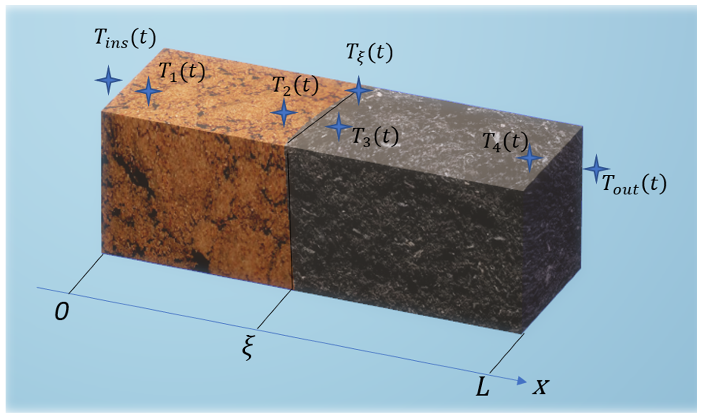
After the solution to the direct problem is received, we may pose the inverse problem and demonstrate its solution algorithm. The formulation of our inverse problem is that in using the measured temperature values at seven points, as indicated in Figure 1 below, it is necessary to determine the values of eight thermo-physical parameters and one geometrical characteristic of the two-layered medium terrain. We write two sets of parameters, noting that the geometrical constant $\xi$ will be evaluated by both sub-domain problems simultaneously due to contact Condition (5):

$$\{\begin{array}{c}{\pi }_1=\left\{{\rho }_1, c_p{}_1, h_{ins}, k_1, \xi \right\},\\ {\pi }_2=\left\{{\rho }_2, c_p{}_2, h_{out}, k_2, \xi \right\}.\end{array}$$

(91)

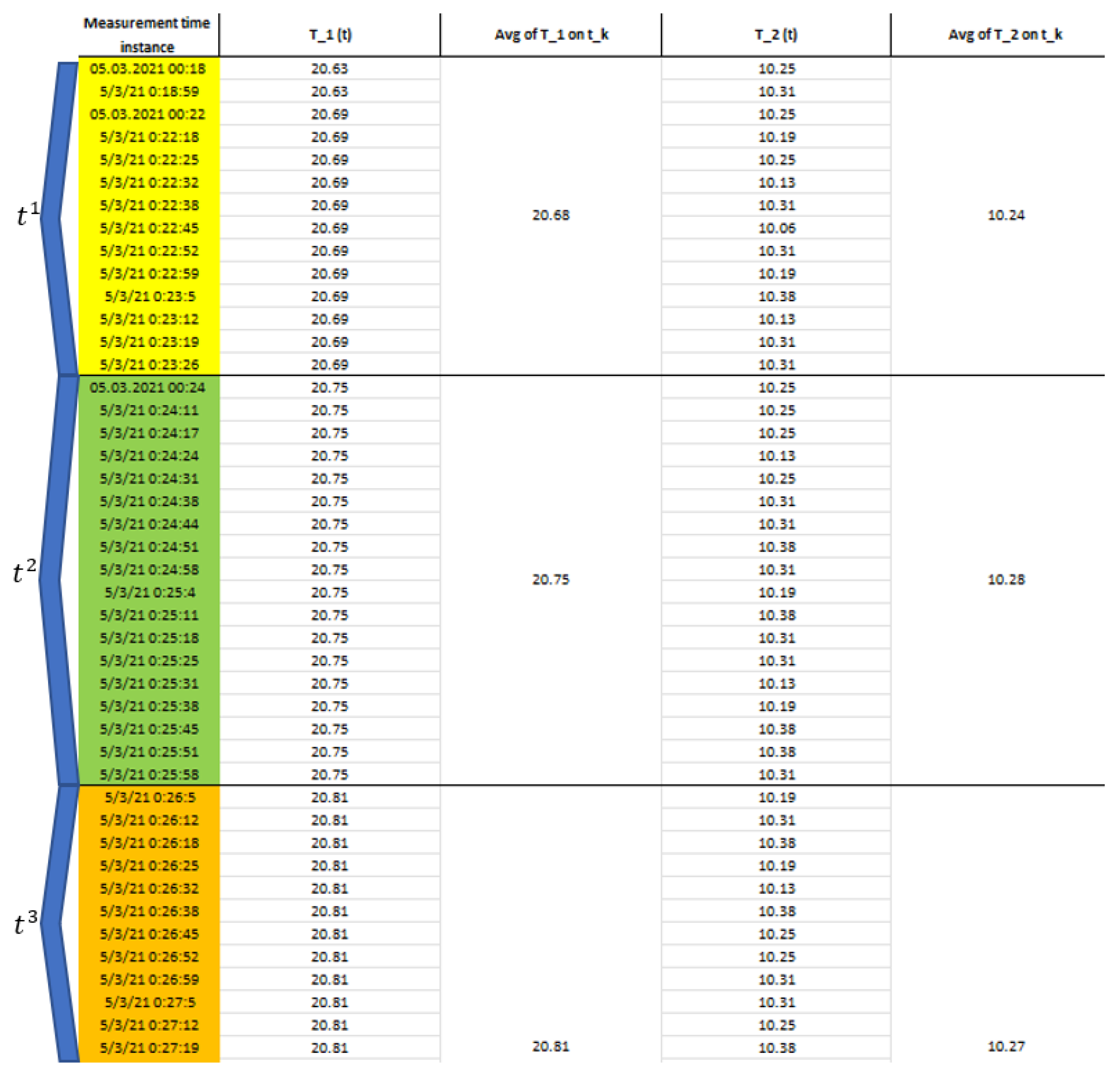
Firstly, to determine the coefficients we shall specify a time partition, where ambient temperature is constant, i.e., with fluctuations that may be neglected in order to obtain homogeneous boundary conditions, as illustrated on Figure 2 below.

Afterwards, on each such time sub-domain $t^k\in \left(t_i, t_{i+1}\right)$ we evaluate iteratively by one parameter from our ${\pi }_1$ and ${\pi }_2$. To solve the system of nonlinear equations that we receive upon the determination of unknown parameters, we employ numerical iterative algorithms, such as the Newton’s method, dichotomy or the simple iterations method [24,25,26,27]. We estimate each parameter iteratively and perform Algorithm 1 to compute the temperature field on each iteration until we reach the following stop criterion:

$$|u\left(x_m,t\right)-T_{g_m}\left(t\right)|\le \epsilon .$$

(92)

where $\epsilon$ is predefined accuracy, $x_m$ is the measurement device position, and $T_{g_m}\left(t\right)$ is the measured temperature. By using the measurements at the first indicated point, we construct the following functions to be minimized; it could be investigated whether the proposed functions perceive the local convex properties. However, in a case of a non-convex function, we may utilize the least square method to solve an equivalent convex extreme problem:

$$\{\begin{array}{cc}{T}_1\left(t^k\right)-{\displaystyle \sum _{n=1}^{\infty }}{B}_n{e}^{-{\lambda }_n\frac{k_1}{{\rho }_1{c}_{p_1}}{t}^k}{X}_n\left(0\right)+\gamma =f\left({\rho }_1\right),& \\ T_1\left(t^{k+1}\right)-{\displaystyle \sum _{n=1}^{\infty }}{B}_n{e}^{-{\lambda }_n\frac{k_1}{{\rho }_1{c}_{p_1}}{t}^{k+1}}{X}_n\left(0\right)+\gamma =f\left( c_{p_1}\right),& \\ & \to \mathit{min}\\ T_1\left(t^{k+2}\right)-{\displaystyle \sum _{n=1}^{\infty }}{B}_n{e}^{-{\lambda }_n\frac{k_1}{{\rho }_1{c}_{p_1}}{t}^{k+2}}{X}_n\left(0\right)+\gamma =f\left(h_{\mathit{ins}}\right),& \\ T_1\left(t^{k+3}\right)-{\displaystyle \sum _{n=1}^{\infty }}{B}_n{e}^{-{\lambda }_n\frac{k_1}{{\rho }_1{c}_{p_1}}{t}^{k+3}}{X}_n\left(0\right)+\gamma =f(k_1).& \end{array}$$

(93)

After we evaluate these four parameters of the first set ${\pi }_1$, we additionally clarify these values via the same optimization problem from the system with measurements received from the second device, with $x_2$ being the position of the second measuring device:

$$\{\begin{array}{cc}{T}_2\left(t^k\right)-{\displaystyle \sum _{n=1}^{\infty }}{B}_n{e}^{-{\lambda }_n\frac{k_1}{{\rho }_1{c}_{p_1}}{t}^k}{X}_n\left(x_2\right)+\gamma +{\gamma }_1{x}_2=f\left({\rho }_1\right),& \\ T_2\left(t^{k+1}\right)-{\displaystyle \sum _{n=1}^{\infty }}{B}_n{e}^{-{\lambda }_n\frac{k_1}{{\rho }_1{c}_{p_1}}{t}^{k+1}}{X}_n\left(x_2\right)+\gamma +{\gamma }_1{x}_2=f\left(c_{p_1}\right),& \\ & \to \mathit{min}\\ T_2\left(t^{k+2}\right)-{\displaystyle \sum _{n=1}^{\infty }}{B}_n{e}^{-{\lambda }_n\frac{k_1}{{\rho }_1{c}_{p_1}}{t}^{k+2}}{X}_n\left(x_2\right)+\gamma +{\gamma }_1{x}_2=f\left(h_{\mathit{ins}}\right),& \\ T_2\left(t^{k+3}\right)-{\displaystyle \sum _{n=1}^{\infty }}{B}_n{e}^{-{\lambda }_n\frac{k_1}{{\rho }_1{c}_{p_1}}{t}^{k+3}}{X}_n\left(x_2\right)+\gamma +{\gamma }_1{x}_2=f(k_1).& \end{array}$$

(94)

In the same step, we go to the next device measurements and perform the same procedure for another four parameters of our system ${\pi }_2$:

$$\{\begin{array}{cc}{T}_3\left(t^k\right)-{\displaystyle \sum _{n=1}^{\infty }}{D}_n{e}^{-{\mu }_2\frac{k_2}{{\rho }_2{c}_{p_2}}{t}^k}\mathit{sin}\left({\mu }_2{x}_3\right)+\beta +{\beta }_1{x}_3=f\left({\rho }_2\right),& \\ T_3\left(t^{k+1}\right)-{\displaystyle \sum _{n=1}^{\infty }}{D}_n{e}^{-{\mu }_2\frac{k_2}{{\rho }_2{c}_{p_2}}{t}^{k+1}}\mathit{sin}\left({\mu }_2{x}_3\right)+\beta +{\beta }_1{x}_3=f\left(c_{p_2}\right),& \\ & \to \mathit{min}\\ T_3\left(t^{k+2}\right)-{\displaystyle \sum _{n=1}^{\infty }}{D}_n{e}^{-{\mu }_2\frac{k_2}{{\rho }_2{c}_{p_2}}{t}^{k+2}}\mathit{sin}\left({\mu }_2{x}_3\right)+\beta +{\beta }_1{x}_3=f\left(h_{\mathit{out}}\right),& \\ T_3\left(t^{k+3}\right)-{\displaystyle \sum _{n=1}^{\infty }}{D}_n{e}^{-{\mu }_2\frac{k_2}{{\rho }_2{c}_{p_2}}{t}^{k+3}}\mathit{sin}\left({\mu }_2{x}_3\right)+\beta +{\beta }_1{x}_3=f(k_2).& \end{array}$$

(95)

We also perform the same clarification via the last, fourth measurement device, constructing the following system:

$$\{\begin{array}{cc}{T}_4\left(t^k\right)-{\displaystyle \sum _{n=1}^{\infty }}{D}_n{e}^{-{\mu }_2\frac{k_2}{{\rho }_2{c}_{p_2}}{t}^k}\mathit{sin}\left({\mu }_2{x}_4\right)+\beta +{\beta }_1{x}_4=f\left({\rho }_2\right),& \\ T_4\left(t^{k+1}\right)-{\displaystyle \sum _{n=1}^{\infty }}{D}_n{e}^{-{\mu }_2\frac{k_2}{{\rho }_2{c}_{p_2}}{t}^{k+1}}\mathit{sin}\left({\mu }_2{x}_4\right)+\beta +{\beta }_1{x}_4=f\left(c_{p_2}\right),& \\ & \to \mathit{min}\\ T_4\left(t^{k+2}\right)-{\displaystyle \sum _{n=1}^{\infty }}{D}_n{e}^{-{\mu }_2\frac{k_2}{{\rho }_2{c}_{p_2}}{t}^{k+2}}\mathit{sin}\left({\mu }_2{x}_4\right)+\beta +{\beta }_1{x}_4=f\left(h_{\mathit{out}}\right),& \\ T_4\left(t^{k+3}\right)-{\displaystyle \sum _{n=1}^{\infty }}{D}_n{e}^{-{\mu }_2\frac{k_2}{{\rho }_2{c}_{p_2}}{t}^{k+3}}\mathit{sin}\left({\mu }_2{x}_4\right)+\beta +{\beta }_1{x}_4=f(k_2).& \end{array}$$

(96)

At each iteration we observe the changes of all system parameters, performing evaluation via Algorithm 1 through Formulas (86)–(90). However, to determine the geometrical parameter, we implement the contact condition, obtaining another convex function subjected to minimization:

$${{\displaystyle \sum }}_{n=1}^{\infty }{D}_n{e}^{-{\lambda }_n\frac{k_2}{{\rho }_2{c}_{p_2}}{t}^{k+5}}\mathit{sin}\left[{\mu }_2\xi \right]+\beta +{\beta }_1\xi -{{\displaystyle \sum }}_{n=1}^{\infty }{B}_n{e}^{-{\lambda }_n\frac{k_1}{{\rho }_1{c}_{p_1}}{t}^{k+5}}{X}_n\left(\xi \right)+\gamma +{\gamma }_1\xi =f\left(\xi \right)\to min$$

(97)

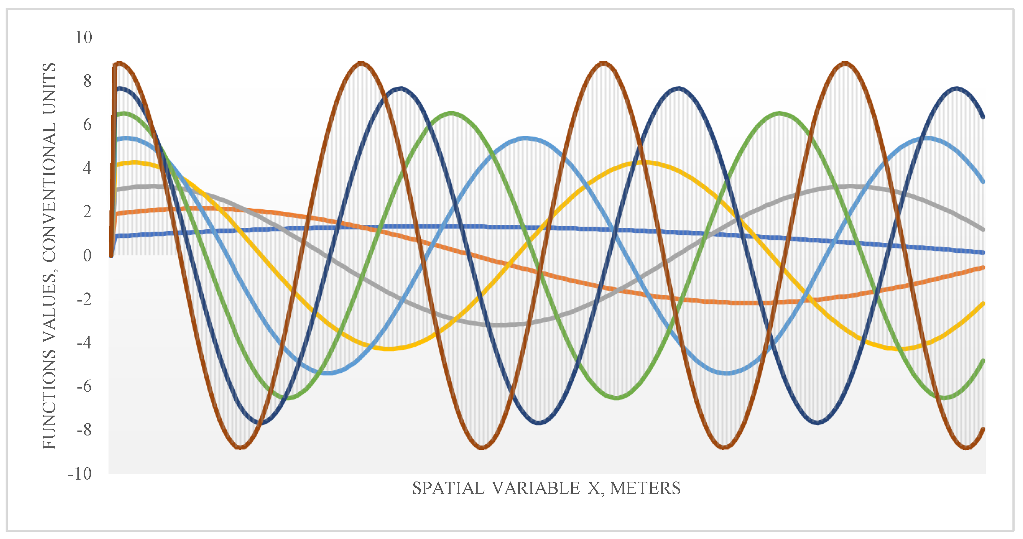
The computational algorithm consists of suitably selected procedures for the temperature measurements, avoiding high levels of fluctuation of more than 0.1% in degrees. Afterwards, we solve Systems (93)–(97) via three different numerical methods: Newton’s, dichotomy and simple iterations, checking at each iteration the criterion (92) that indicates the level of correspondence of the seeking parameters. We present below the separate changes along each iteration of the computed coefficients. Also, Figure 3 below indicates the eigenfunctions on the root of the transcendental equation perceiving the orthonormal behaviour:

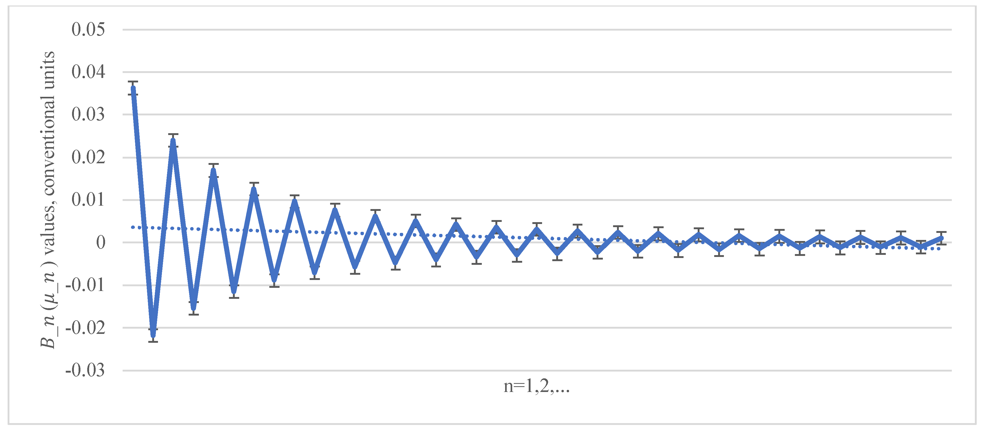
The uniform equicontinuity of the Fourier coefficients (89) indicates uniform convergency of the posed norm (88) by the Arzelà–Ascoli theorem [28,29,30], which can be verified via the Cauchy sequence behaviour [31,32,33] observed in the plot below in Figure 4:

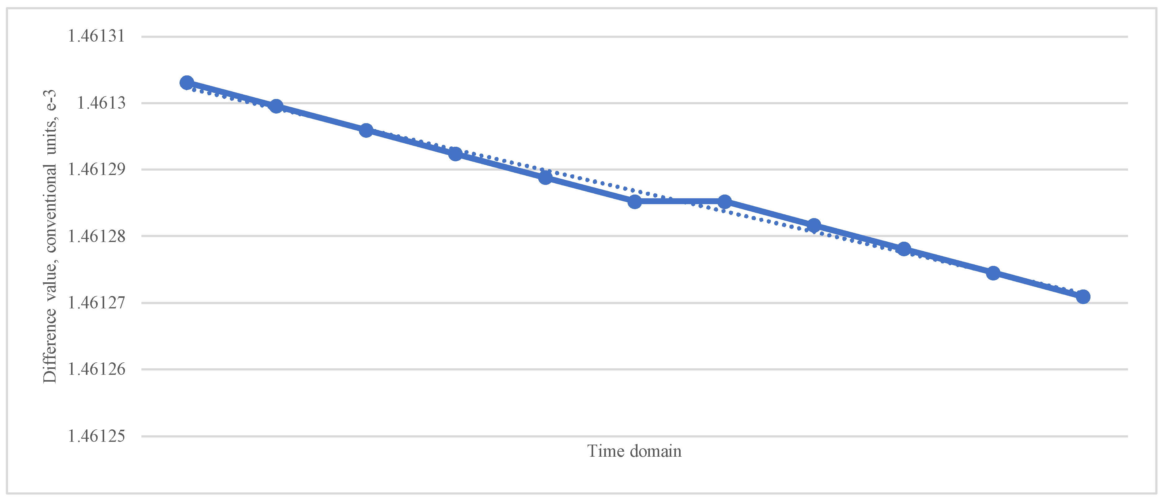
At the same time, we observe the decrease of temperatures’ differences, indicating monotonous convergency in the posed criterion (92) in the plot below in Figure 5.

The set of values ${\pi }_1$ over iterations demonstrate gradual estimation, and we may observe that the initial approximation was overestimated.

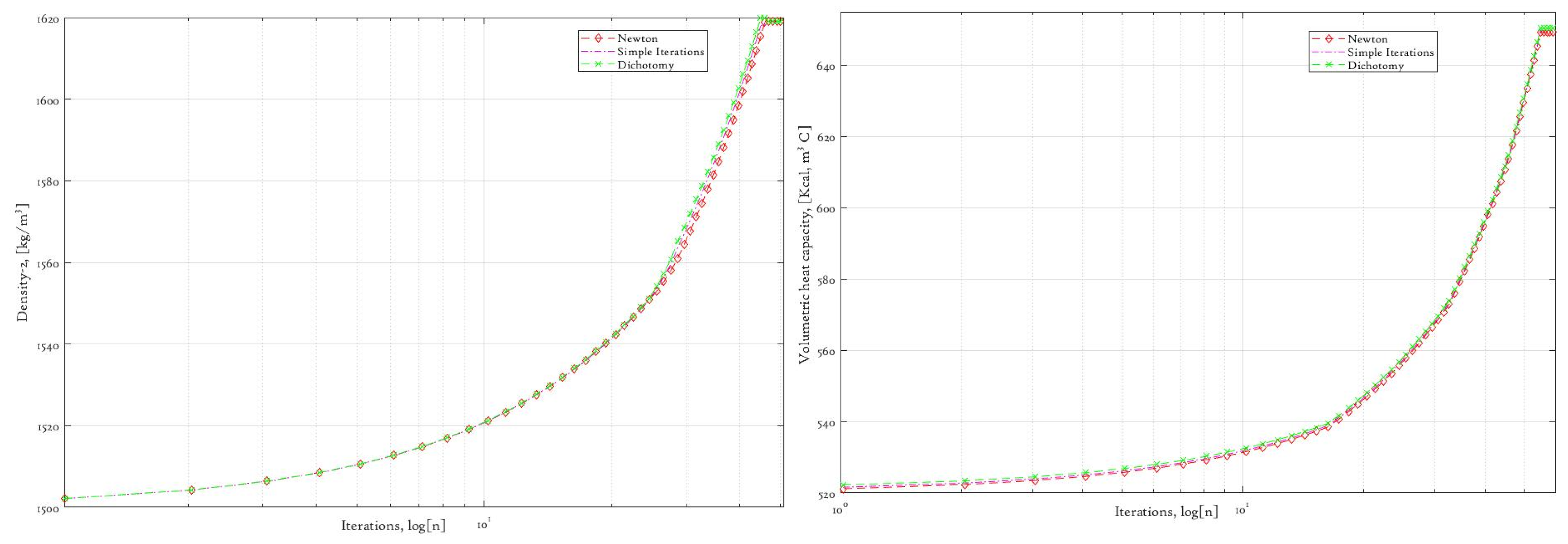
As can be observed from Figure 6, the initial approximations that we chose were overestimated; thus, through the iterations we obtain a gradual decrease in values until we reach stationary values at several final iterations. Although we see small differences in the convergency rate that depend entirely on the numerical method that we choose, it is a matter of fact that the final results are still the same.

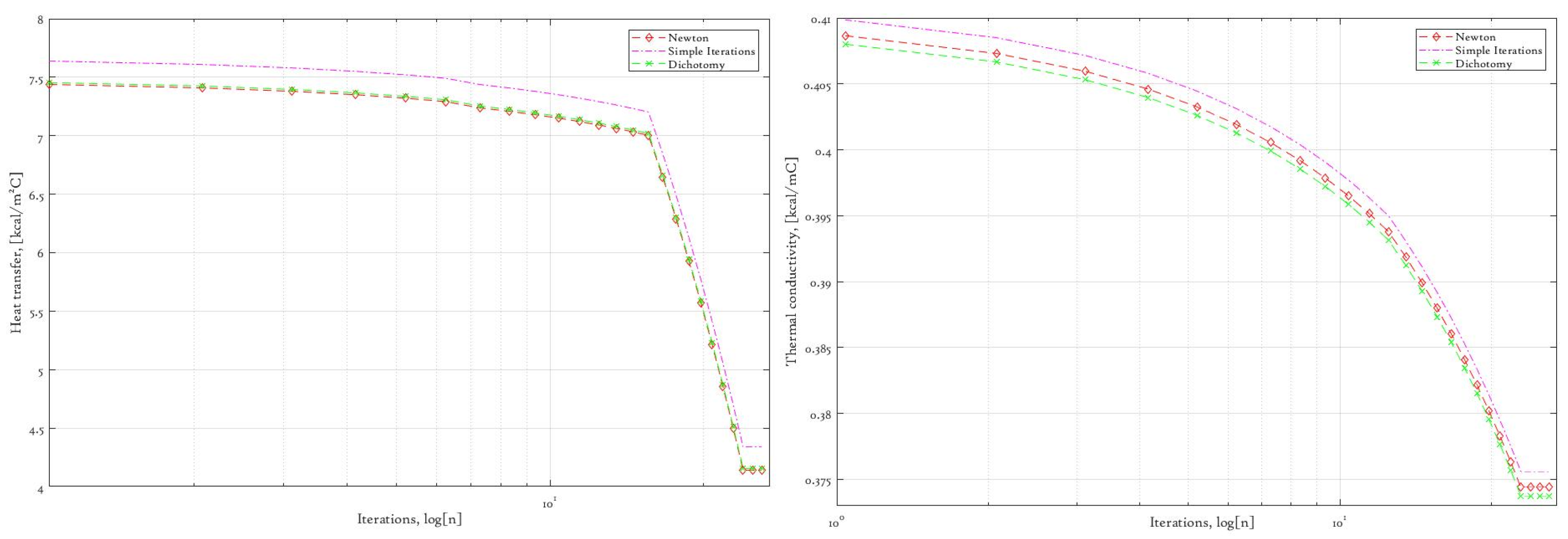
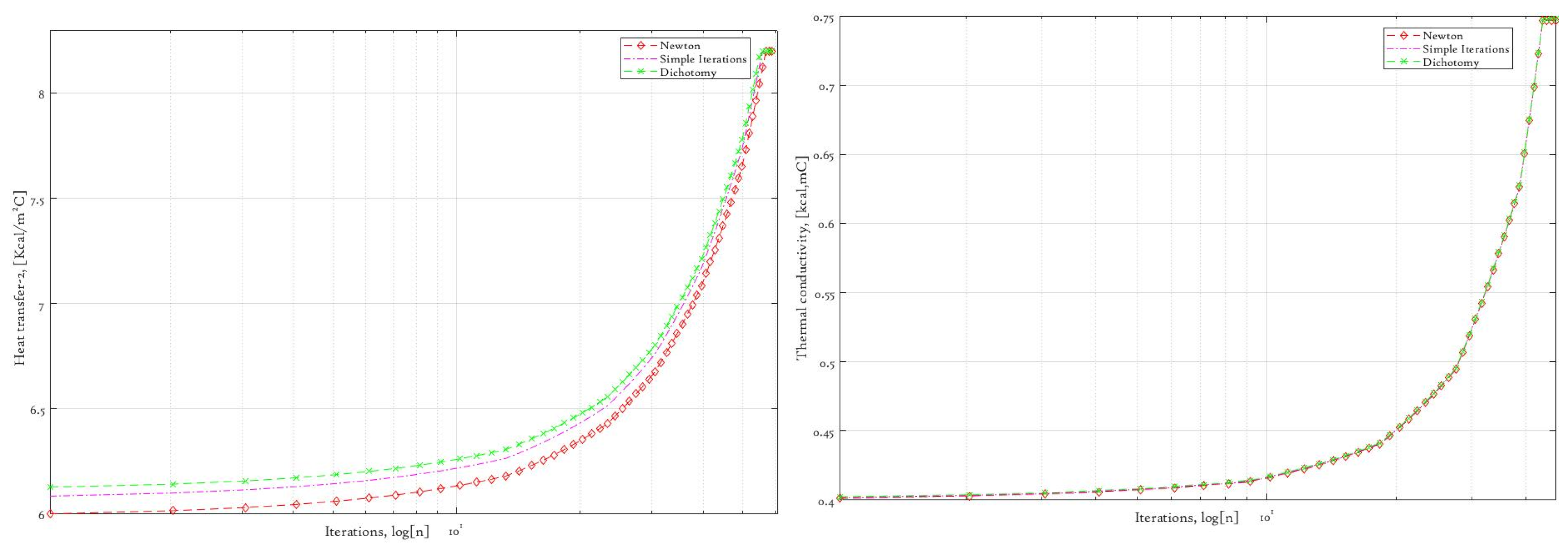
As we also observe in Figure 7, from the determination of another two parameters, there is the same gradual decrease over each iteration, with various convergency rates and slight differences in the final result. This occurs due to the low orders of the parameters’ values; it may be regularized by the introduction of higher-order accuracy in stop criterion (92), which will lead increase in the number of iterations. For the computation of the first layer’s four parameters, we use first two systems of Equations (93) and (94), while another two systems of nonlinear Equations (95) and (96) are used for the second part of our parameter set. However, we intentionally present underestimated initial approximations for the second medium layer, observing the following profiles in Figure 8:

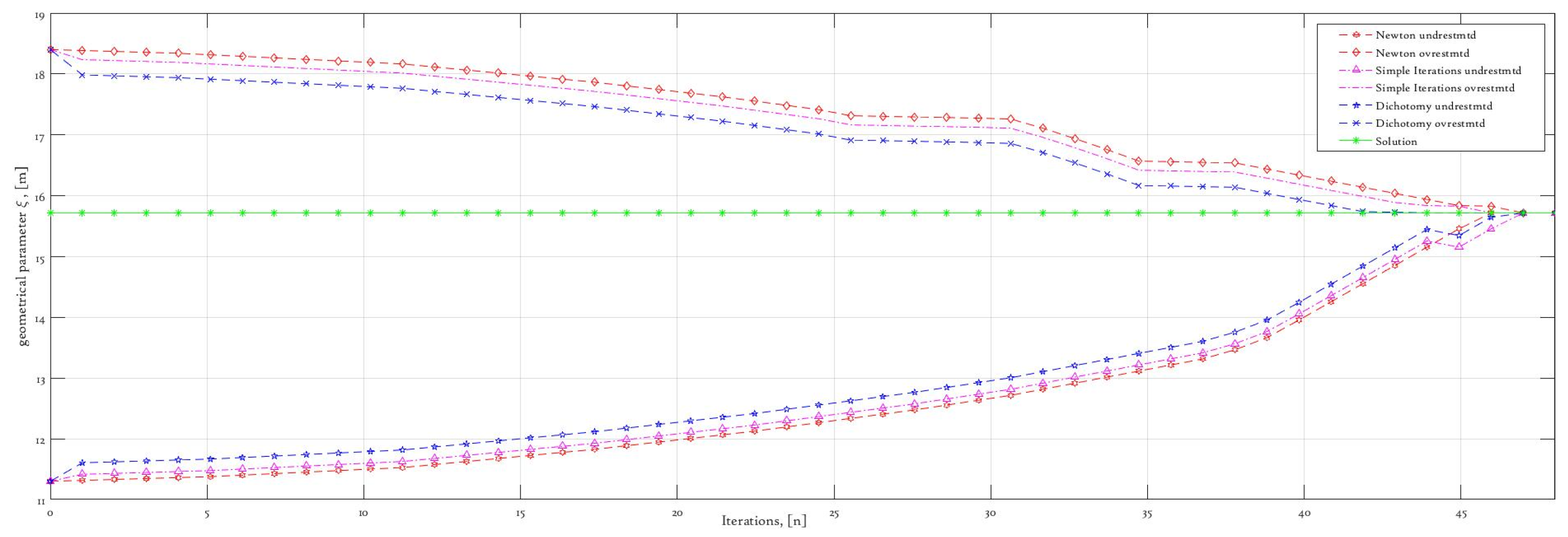
Although the differences in the convergency rate vary over iterations in the second case less in comparison to the first layer parameter estimation procedure, we may connect this observation with the solid decrease in the uncertainty level due to the underestimated initial approximations that we obtain by bounding the above goal function parameters. Still, the matter of the convergency rate may be easily improved by selecting the corresponding iterative approach if certain stability condition constraints are applicable for the posed model [34,35,36,37,38]. Now we demonstrate estimation of the geometrical parameter via iterative Solution (97). We apply the same iterative methods while choosing different initial approximations, selecting them to be both underestimated and overestimated in order to validate the received expressions depicted below in Figure 9:

As can be clearly observed from Figure 9, there is a stable approach for the exact value from both ways, which is achieved via meaningful selection of some physical constraints. Thus, in the case of selecting such constraints sequentially, parameter tunning is not necessary [39]. However, as was reflected by various investigations [40,41,42], the parameter value used for regularized inverse problems is quite critical, as it affects the results and the optimal order of convergency.

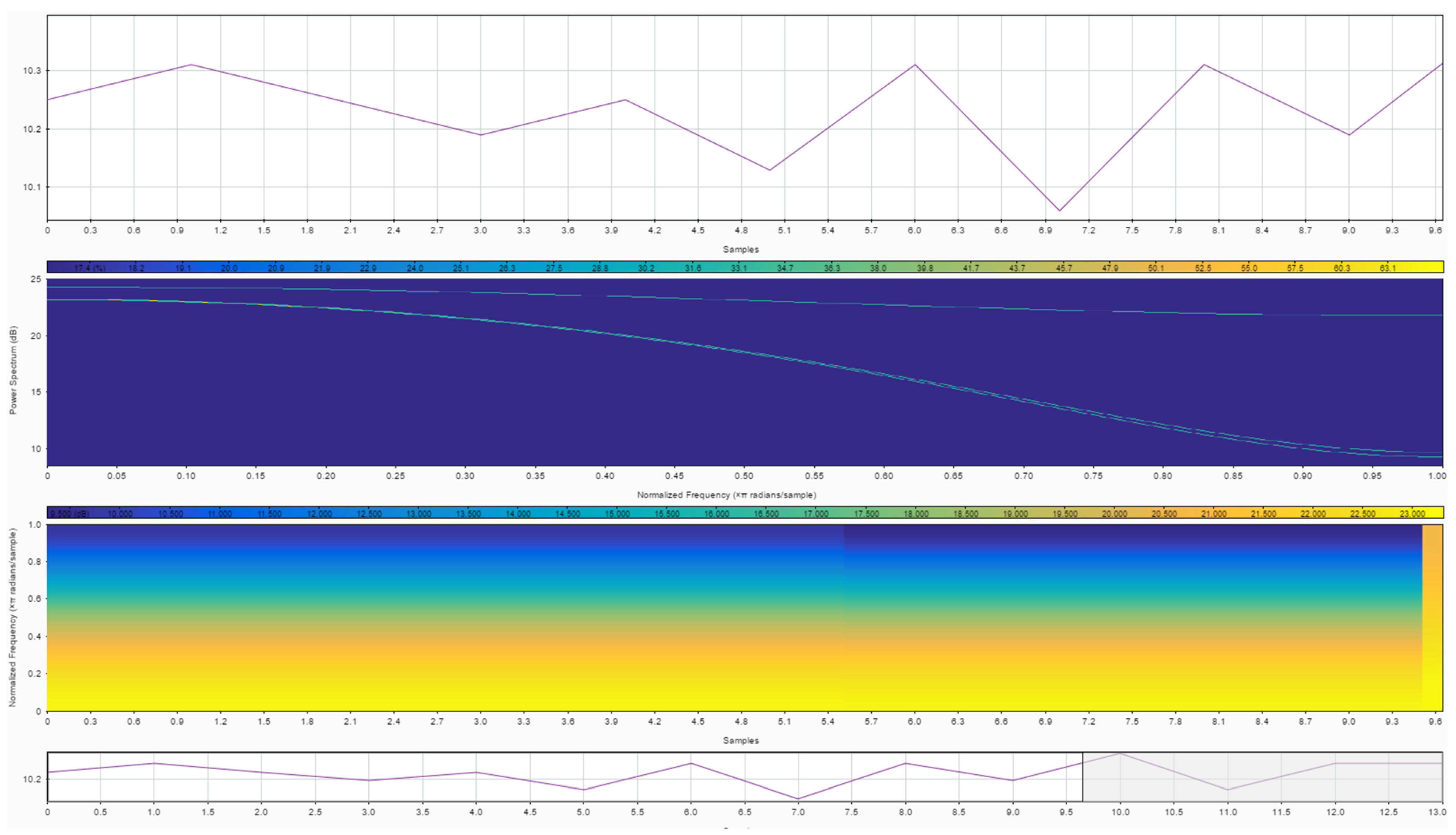
We also investigate the noise simulation as a divergence-free vector field, as the measurements taken with devices include some error during the input process. For that reason, we observe the noise error as:

$$\widetilde{T_{\xi }}=T_{\xi }\left(1+{\breve{\xi }}_n\right).$$

(98)

Here, ${\breve{\xi }}_n$ is the prescribed error of the measuring device taken at a selected point, which could be taken as a smooth-step sigmoid-like interpolation and clamping function, as depicted below in Figure 10.

At the same time, we may extend the prescribed error to an analogue of simplex noise scaling to a higher dimension, reducing the computational cost to $O\left(n^2\right)$ instead of $O\left(n{2}^n\right).$

2. Conclusions

We have demonstrated by received exact analytical expressions that further parameter estimation becomes a more simplified iterative problem. Using derived norms estimations for the eigenfunctions of the governing equations, we obtained expressions for the coefficients of the exact solution for homogenized boundary conditions. Through transfer Formula (86) we extend the received expressions to the original model, and applying Algorithm 1, we obtain computational values for the temperature field. After that, we use our experimentally sampled set of data as an assessment factor to determine all thermophysical parameters via the solution of the nonlinear systems of Equations (93)–(96), keeping the criterion of accuracy (92) at a desirable level through a predefined error upper bound. Furthermore, Expression (97) allows us to determine the geometrical characteristics of the considered domain. Although the posed algorithm was illustrated in two layered media, it is still a matter of small difficulties to extend it for multiple layers due to estimation of eigenfunction norms. However, with homogenized boundary conditions, we may consider various physical positions for equivalent models. The presented algorithm works for both underestimated and overestimated initial approximations. We have derived analytical expressions for the determination of the key physical parameters at the same time, along with the geometrical characteristic. Initially, our relations introduced for the homogenization of the sampled measurements played an essential role in the derivation process of analytical expressions and presented proofs of the posed lemmas. We have constructed the computational algorithm and validated the obtained results in terms of the derived expressions via the comparison of the computed values with the empirically received measurements.

References

1. Bates, O.; Guasch, L.; Strong, G.; Robins, T.C.; Calderon-Agudo, O.; Cueto, C.; Tang, M. A probabilistic approach to tomography and adjoint state methods, with an application to full waveform inversion in medical ultrasound. Inverse Probl. 2022, 38, 045008. [Google Scholar] [CrossRef]
2. Baguer, D.O.; Leuschner, J.; Schmidt, M. Computed tomography reconstruction using deep image prior and learned reconstruction methods. Inverse Probl. 2020, 36, 094004. [Google Scholar] [CrossRef]
3. Gerth, D. A new interpretation of (Tikhonov) regularization. Inverse Probl. 2021, 37, 064002. [Google Scholar] [CrossRef]
4. Gondzio, J.; Lassas, M.; Latva-Äijö, S.M.; Siltanen, S.; Zanetti, F. Material-separating regularizer for multi-energy x-ray tomography. Inverse Probl. 2022, 38, 025013. [Google Scholar] [CrossRef]
5. Hostos, J.C.Á.; Fachinotti, V.D.; Peralta, I. Computational design of thermo-mechanical metadevices using topology optimization. Appl. Math. Model. 2021, 90, 758–776. [Google Scholar] [CrossRef]
6. Fernandes, A.P.; dos Santos, M.B.; Guimarães, G. An analytical transfer function method to solve inverse heat conduction problems. Appl. Math. Model. 2015, 39, 6897–6914. [Google Scholar] [CrossRef]
7. Qiu, L.; Lin, J.; Wang, F.; Qin, Q.-H.; Liu, C.-S. A homogenization function method for inverse heat source problems in 3D functionally graded materials. Appl. Math. Model. 2021, 91, 923–933. [Google Scholar] [CrossRef]
8. Mu, X.; Cheng, H.; Xu, Q.; Liu, G. Stably numerical solving inverse boundary value problem for data assimilation. Appl. Math. Model. 2020, 82, 825–835. [Google Scholar] [CrossRef]
9. Yang, L.; Deng, Z.-C.; Yao, B.; Wang, L.B. An inverse problem of determining the shape of rotating body by temperature measurements. Appl. Math. Model. 2018, 59, 464–482. [Google Scholar] [CrossRef]
10. Gostimirovic, M.; Sekulic, M.; Trifunovic, M.; Madic, M.; Rodic, D. Stability analysis of the inverse heat transfer problem in the optimization of the machining process. Appl. Therm. Eng. 2021, 195, 117174. [Google Scholar] [CrossRef]
11. Zálešák, M.; Charvát, P.; Klimeš, L. Identification of the effective heat capacity–temperature relationship and the phase change hysteresis in PCMs by means of an inverse heat transfer problem solved with metaheuristic methods. Appl. Therm. Eng. 2021, 197, 117392. [Google Scholar] [CrossRef]
12. Tansri, K.; Chansangiam, P. Conjugate Gradient Algorithm for Least-Squares Solutions of a Generalized Sylvester-Transpose Matrix Equation. Symmetry 2022, 14, 1868. [Google Scholar] [CrossRef]
13. Sokhal, S.; Verma, S.R. A Fourier wavelet series solution of partial differential equation through the separation of variables method. Appl. Math. Comput. 2021, 388, 125480. [Google Scholar] [CrossRef]
14. Meyer, T. Improvement of the exact analytical solutions for combined heat and mass transfer problems obtained with the Fourier method. Int. J. Refrig. 2014, 43, 133–142. [Google Scholar] [CrossRef]
15. Shi, Y.; Ding, S.; Qiu, T.; Liu, C.; Zhang, S. Bi-Fo time scaling method in the numerical simulation of transient conjugate heat transfer. Propuls. Power Res. 2021, 10, 209–223. [Google Scholar] [CrossRef]
16. Singh, S.; Kumar, D.; Rai, K.N. Analytical solution of Fourier and non-Fourier heat transfer in longitudinal fin with internal heat generation and periodic boundary condition. Int. J. Therm. Sci. 2018, 125, 166–175. [Google Scholar] [CrossRef]
17. Lin, J.; Zhang, Y. Sergiy Reutskiy, A semi-analytical method for 1D, 2D and 3D time fractional second order dual-phase-lag model of the heat transfer. Alex. Eng. J. 2021, 60, 5879–5896. [Google Scholar] [CrossRef]
18. Bi, W.; Wan, J.; Chen, J.; Zhang, X. Quasi-analytical solution to the problem of heat transfer by vortex flow based on self-similarity. Int. Commun. Heat Mass Transf. 2022, 134, 106005. [Google Scholar] [CrossRef]
19. Li, B.; Zhang, J.; Cheng, J.; Yan, H.; Liu, H. An analytical solution to periodical heat transfer problems of multilayer rocks for thermal energy storage in underground mines. J. Energy Storage 2022, 50, 104320. [Google Scholar] [CrossRef]
20. Ramos, J.I. Analytical and numerical solutions to some one-dimensional relativistic heat equations. Appl. Math. Model. 2017, 46, 181–202. [Google Scholar] [CrossRef]
21. Song, G.-J.; Wang, Q.-W.; Yu, S.-W. Cramer’s rule for a system of quaternion matrix equations with applications. Appl. Math. Comput. 2018, 336, 490–499. [Google Scholar] [CrossRef]
22. Song, G.-J.; Wang, Q.-W. Condensed Cramer rule for some restricted quaternion linear equations. Appl. Math. Comput. 2011, 218, 3110–3121. [Google Scholar] [CrossRef]
23. Kyrchei, I. Analogs of Cramer’s rule for the minimum norm least squares solutions of some matrix equations. Appl. Math. Comput. 2012, 218, 6375–6384. [Google Scholar] [CrossRef]
24. Sulaiman, I.M.; Mamat, M.; Malik, M.; Nisar, K.S.; Elfasakhany, A. Performance analysis of a modified Newton method for parameterized dual fuzzy nonlinear equations and its application. Results Phys. 2022, 33, 105140. [Google Scholar] [CrossRef]
25. Candelario, G.; Cordero, A.; Torregrosa, J.R.; Vassileva, M.P. An optimal and low computational cost fractional Newton-type method for solving nonlinear equations. Appl. Math. Lett. 2022, 124, 107650. [Google Scholar] [CrossRef]
26. Arias, C.A.; Martínez, H.J.; Pérez, R. Global inexact quasi-Newton method for nonlinear system of equations with constraints. Appl. Numer. Math. 2020, 150, 559–575. [Google Scholar] [CrossRef]
27. Kumar, M.; Singh, A.K.; Srivastava, A. Various Newton-type iterative methods for solving nonlinear equations. J. Egypt. Math. Soc. 2013, 21, 334–339. [Google Scholar] [CrossRef] [Green Version]
28. Zhenhai, L.; Szántó, I. Inverse coefficient problems for parabolic hemivariational inequalities. Acta Math. Sci. 2011, 31, 1318–1326. [Google Scholar] [CrossRef]
29. Ellabib, A.; Ouakrim, Y. Inverse problem for a class of nonlinear elliptic equations with entropy solution. Nonlinear Anal. Real World Appl. 2019, 46, 137–156. [Google Scholar] [CrossRef]
30. Chen, P.; Wang, R.; Zhang, X. Long-time dynamics of fractional nonclassical diffusion equations with nonlinear colored noise and delay on unbounded domains. Bull. Des Sci. Math. 2021, 173, 103071. [Google Scholar] [CrossRef]
31. Alderremy, A.A.; Shah, R.; Iqbal, N.; Aly, S.; Nonlaopon, K. Fractional Series Solution Construction for Nonlinear Fractional Reaction-Diffusion Brusselator Model Utilizing Laplace Residual Power Series. Symmetry 2022, 14, 1944. [Google Scholar] [CrossRef]
32. Hobiny, A.; Alzahrani, F.; Abbas, I.; Marin, M. The Effect of Fractional Time Derivative of Bioheat Model in Skin Tissue Induced to Laser Irradiation. Symmetry 2020, 12, 602. [Google Scholar] [CrossRef] [Green Version]
33. Nachaoui, A.; Nachaoui, M.; Chakib, A.; Hilal, M.A. Some novel numerical techniques for an inverse Cauchy problem. J. Comput. Appl. Math. 2021, 381, 113030. [Google Scholar] [CrossRef]
34. Liu, C.; Han, X.; Zhang, L. Unconditional convergence of iterative approximation methods. Eng. Anal. Bound. Elem. 2021, 126, 161–168. [Google Scholar] [CrossRef]
35. Mittal, G.; Giri, A.K. Convergence rates for iteratively regularized Gauss–Newton method subject to stability constraints. J. Comput. Appl. Math. 2022, 400, 113744. [Google Scholar] [CrossRef]
36. Lin, Y.; Bao, L.; Wu, Q. On the convergence rate of an iterative method for solving nonsymmetric algebraic Riccati equations. Comput. Math. Appl. 2011, 62, 4178–4184. [Google Scholar] [CrossRef] [Green Version]
37. Kia, H.A.; Zangian, M.; Minuchehr, A.; Zolfaghari, A. An improved convergence rate for the prompt α eigenvalue calculation in α-k iteration methods. Ann. Nucl. Energy 2018, 118, 15–25. [Google Scholar] [CrossRef]
38. Guo, C.-H.; Lin, W.-W. Convergence rates of some iterative methods for nonsymmetric algebraic Riccati equations arising in transport theory. Linear Algebra Appl. 2010, 432, 283–291. [Google Scholar] [CrossRef] [Green Version]
39. Naqeeb, M.; Hussain, A.; Alghamdi, A.M. An Improved Regularity Criterion for the 3D Magnetic Bénard System in Besov Spaces. Symmetry 2022, 14, 1918. [Google Scholar] [CrossRef]
40. Liao, H.; Ma, H. Error estimate of a Legendre-Galerkin Chebyshev collocation method for a class of parabolic inverse problem. Appl. Numer. Math. 2021, 170, 179–189. [Google Scholar] [CrossRef]
41. Alzahrani, F.; Hobiny, A.; Abbas, I.; Marin, M. An Eigenvalues Approach for a Two-Dimensional Porous Medium Based Upon Weak, Normal and Strong Thermal Conductivities. Symmetry 2020, 12, 848. [Google Scholar] [CrossRef]
42. Marin, M.; Hobiny, A.; Abbas, I. The Effects of Fractional Time Derivatives in Porothermoelastic Materials Using Finite Element Method. Mathematics 2021, 9, 1606. [Google Scholar] [CrossRef]
Figure 1. Experimental design schematic overview.
Symmetry 14 02248 g001
Figure 2. Decomposition of the time-domain scheme.
Symmetry 14 02248 g002
Figure 3. Eigenfunction values distribution for posed direct problem.
Symmetry 14 02248 g003
Figure 4. Fourier coefficient B n ( μ n ) for different roots of transcendental equation solutions.
Symmetry 14 02248 g004
Figure 5. Difference values at selected measuring device and evaluated temperatures through iterations.
Symmetry 14 02248 g005
Figure 6. Density and volumetric heat capacity estimation.
Symmetry 14 02248 g006
Figure 7. Heat transfer and thermal conductivity estimation.
Symmetry 14 02248 g007
Figure 8. Second layer parameter estimation.
Symmetry 14 02248 g008aSymmetry 14 02248 g008b
Figure 9. Geometrical parameter estimation.
Symmetry 14 02248 g009
Figure 10. Noise analysis for sampled measurements.
Symmetry 14 02248 g010
Publisher’s Note: MDPI stays neutral with regard to jurisdictional claims in published maps and institutional affiliations.